Model selection and parameter estimation in structural dynamics using approximate Bayesian computation

(1)

Model selection and parameter estimation in structural

dynamics using approximate Bayesian computation

Anis Ben Abdessalem

⇑

, Nikolaos Dervilis, David Wagg, Keith Worden

Dynamics Research Group, Department of Mechanical Engineering, University of Sheffield, Mappin Street, Sheffield S1 3JD, United Kingdom

a r t i c l e i n f o

Article history: Received 9 March 2017

Received in revised form 14 June 2017 Accepted 17 June 2017

Keywords: Model selection Parameter estimation

Approximate Bayesian computation Sequential Monte Carlo

Nonlinearity

a b s t r a c t

This paper will introduce the use of the approximate Bayesian computation (ABC) algo-rithm for model selection and parameter estimation in structural dynamics. ABC is a likelihood-free method typically used when the likelihood function is either intractable or cannot be approached in a closed form. To circumvent the evaluation of the likelihood function, simulation from a forward model is at the core of the ABC algorithm. The algo-rithm offers the possibility to use different metrics and summary statistics representative of the data to carry out Bayesian inference. The efficacy of the algorithm in structural dynamics is demonstrated through three different illustrative examples of nonlinear sys-tem identification: cubic and cubic-quintic models, the Bouc-Wen model and the Duffing oscillator. The obtained results suggest that ABC is a promising alternative to deal with model selection and parameter estimation issues, specifically for systems with complex behaviours.

Ó2017 The Author(s). Published by Elsevier Ltd. This is an open access article under the CC BY license (http://creativecommons.org/licenses/by/4.0/).

1. Introduction

In many areas of engineering and science, researchers or engineers are dealing with model selection and comparison issues, in particular when several competing models are consistent with the selection criteria and could potentially explain the data reasonably well. In most cases, selecting the most likely model among a set of competing models may be quite chal-lenging, often requiring a deep understanding of the physics involved. Several methods have been proposed in the literature, and arguably the most popular currently is the Bayesian approach. During the last two decades, the Bayesian approach has been successfully implemented in many areas to deal with model selection and parameter estimation issues. Compared with other statistical methods, Bayesian theory provides a comprehensive and coherent framework, and a generally applicable way to make inference about models from data. The reader can refer to the following references[1–6]and the references therein, where many varied examples illustrating the use of the Bayesian method are investigated. In the Bayesian paradigm, the best model is the one that satisfies the parsimony principle, which means the right balance between complexity of the model and goodness-of-fit. Given a number of potential models, and one or more data sets, model selection should identify the model structure and the set of parameters that may explain the data best, while simultaneously penalising overly-complex models. Different methods have been proposed in the literature for model selection based on the Bayes theory; the most popular is reversible-jump Markov chain Monte Carlo (RJ-MCMC) [7]. However, the implementation of the RJ-MCMC algorithm is quite challenging. This is because when one deals with a large number of models with different

http://dx.doi.org/10.1016/j.ymssp.2017.06.017

0888-3270/Ó2017 The Author(s). Published by Elsevier Ltd.

This is an open access article under the CC BY license (http://creativecommons.org/licenses/by/4.0/). ⇑ Corresponding author.

E-mail address:[email protected](A. Ben Abdessalem).

Contents lists available atScienceDirect

Mechanical Systems and Signal Processing

(2)

dimensionalities, the algorithm needs to define a so-called ‘dimension-matching’ mapping law which requires additional computation. The reader is referred to[7]for details. Bayes factors[8]have been considered for a long time as the standard tools for performing Bayesian model comparison; however, these provide only a relative comparison of competing models, not the absolute values of their posterior probabilities.

Sandhu et al.[5]have proposed the use of the Metropolis-Hastings (MH) MCMC simulation and nonlinear filtering. Par-ticle filters as the sequential importance sampling/resampling (SIS/SIR)[9]could be used to make model selection as shown in[10]. More traditional statistical methods such as the Akaike Information Criterion (IC), the Bayesian IC or the deviance IC have been extensively used and investigated in the literature also[11–14]. Essentially, the evaluation of those metrics is based on the maximum likelihood estimate and a penalty term to penalise complex models (complexity is measured usually by the number of parameters in the model). In those methods, the marginal likelihood estimation is undertaken for each model separately, and then these results are used to compute the plausibility of each model. This may be a problem, typically when one deals with a large number of competing models composed of a large number of parameters. Moreover, in the sta-tistical methods based on the ICs, the likelihood is supposed to be very peaked, however, in problems with different types of nonlinearities, the density may be non-Gaussian (e.g., bimodal, multimodal or heavily skewed). In such cases, the ICs cannot be used to compare the candidate models, and this limits their widespread use. Another alternative to deal with model selec-tion and parameter estimaselec-tion is to use the nested sampling (NS) method proposed by Skilling[15,16]. The algorithm works by transforming the multidimensional parameter space integral into a one dimensional integral where classical numerical approximation techniques to estimate the area under a function can be applied. The algorithm has been successfully applied in various research areas[17,18].

The diversity of the methodologies proposed in the literature reflects the complexity of the model selection task; more-over, it shows that there is no universal method that can be used in any circumstances. The choice of the suitable method depends mainly on the available data to conduct Bayesian inference. In this paper, the use of the approximate Bayesian com-putation (ABC) algorithm is introduced as a promising alternative to deal with model selection and parameter estimation. Compared with the methods above, the ABC is more straightforward and general in the sense that there is no need to eval-uate any extra criterion to discriminate between candidate models, and the inference can be performed through any suitable metric to assess the similarity between the observed and simulated data, circumventing the problem of an intractable like-lihood function and the Gaussianity assumption which cannot not always be guaranteed. Moreover, in structural dynamics with complex nonlinearity types, it is often the case that the hypothesis of Gaussianity is not guaranteed. Another major advantage offered by the ABC algorithm is its independence of the dimensionality of the competing models; ABC jumps between the different model spaces without the need of any mapping function to be defined, which is a major benefit in dealing with larger numbers of models. In practice, the ABC algorithm compares the competing models simultaneously, and eliminates progressively the least likely models, to converge to the most plausible one(s). The widespread use of ABC in several fields, and its efficiency to deal with model selection and parameter estimation, simultaneously motivated the cur-rent authors to investigate more the capability of the ABC to infer complex nonlinear systems in structural dynamics. The algorithm shows some attractive properties, including its flexibility to use different kinds of metrics to make system infer-ence and its ability to explore both model and parameter spaces efficiently. The flexibility offered by the ABC algorithm is of paramount importance, as in some circumstances, the likelihood function cannot be analytically formulated or even be approached using approximate methods. Therefore, ABC by its flexibility makes inference possible for many challenging problems.

During the last decade, the ABC algorithm has been applied in many areas for both levels of inference (parameter and model): genetics[19], biology[20,21]and psychology[22]. The rapid developments and continuous improvements of the ABC algorithm attracted many other areas, and recently it has been introduced in structural dynamics by the authors for model selection[23]and parameter estimation in[24]. In[24], the authors show that the combination of the ABC principle with the subset simulation concept[25], introduced to estimate rare events, decreases the computational time and provides the same precision as other variants of the ABC algorithm proposed in the literature such as ABC sequential Monte Carlo (SMC) and ABC-MCMC[26]. In the present work, a more extensive application of ABC-SMC as an efficient tool for model selection and parameter estimation in structural dynamics is presented. ABC appears to be a promising alternative for prac-titioners in structural dynamics to overcome the inference problem of systems with complex behaviours which may undergo bifurcations and/or chaos.

Furthermore, ABC offers the possibility to manage larger datasets and a higher number of competing models with differ-ent dimensionalities, circumvdiffer-enting the limitation of RJ-MCMC. Besides the major advantages mdiffer-entioned so far, the simplic-ity of the ABC method and its capabilsimplic-ity of extending the Bayesian framework to any computer simulation has exponentially increased its popularity. It is worth mentioning that this algorithm already takes into account the parsimony requirement because complex models with larger number of parameters will generate wider posterior distributions. As a result, models with more parameters will be more times below the ABC tolerance threshold, thus promoting simpler models. This property will be investigated in the illustrative examples presented in this work, by considering several models with different degrees of complexity and analysing the behaviour of the algorithm through the inference process.

(3)

2. Approximate Bayesian computation

In the ABC algorithm, the objective is to obtain a good and computationally affordable approximation to the posterior distribution:

p

ðnju;MÞ /fðujn;MÞ

p

ðnjMÞ ð1Þ

whereMis the model based on a set of parametersn;

p

ðnjMÞdenotes the prior distribution over the parameter space and fðujn;MÞis the likelihood of the observed dataufor a given parameter setn.

To overcome the issue of intractable likelihood functions encountered in various real-world problems, the ABC algorithm relies on systematic comparisons between observed and simulated data. The main principle consists of comparing the sim-ulated data,u, with observed datau_{, and accepting simulations if a suitable distance measure between them,}_D_ð_u_; _u_Þ_{, is less} than a specified threshold defined by the user,

e

. The ABC algorithm thus provides a sample from the approximate posterior of the form:

p

ðnju;MÞ

p

eðnju;MÞ / Z

fðujn;MÞIð

D

ðu;uÞ6

e

Þ

p

ðnjMÞdu ð2Þ

whereIðaÞis an indicator function returning unity if the conditionais satisfied and a zero otherwise, when

e

is small enough,

p

eðnju_;_MÞ_{is a good approximation to the true posterior distribution.}

In this work, the ABC-SMC algorithm presented in[27]will be used to make Bayesian inference for model selection and parameter estimation. Generally speaking, the algorithm works as a particle filter which can be used to identify nonlinear dynamical systems[28]. Its mechanism is similar to sequential importance sampling (resampling) SIS/SIR. The SIS/SIR algo-rithm is a Monte Carlo (MC) method that forms the basis for most sequential MC filters developed over the past decades (see, [29–31]). The key idea of ABC-SMC is to represent the required posterior density function by a set of random samples with associated weights. The algorithm converges through a number of intermediate posterior distributions before converging to the optimal approximate posterior distribution satisfying a convergence criterion defined by the user.

Following the scheme shown inAlgorithm 1, for the first iteration, one may start with an arbitrarily large tolerance threshold

e

1to avoid a low acceptance rate and computational inefficacy. One selects directly from the prior distributions

p

ðmÞ and

p

ðnÞ, evaluates the distanceDðu_; _u_Þ_{, and then compares this distance to}

e

1, in order to accept or reject the ðm; nÞselection. This process is repeated untilNparticles distributed over the competing models are accepted. One then assigns equal weights to the accepted particles for each model. For the next iterationsðt>1Þthe tolerance thresholds are set such that

e

1>

e

2> >

e

t. The choice of the final tolerance schedule, denoted here by

e

t, depends mainly on the goals

of the practitioner.

The dynamics by which

e

evolves is a matter of choice, although there is no general prescription; the tolerance threshold can be selected manually or adaptively, based on the distribution of the accepted distances in the previous iteration,t1. For instance, the threshold of the second iteration can be set to thepth_{percentile of the distances in the first iteration. This}

would seem to be the most common choice of tolerance threshold sequence since it is intuitive and simple to define. Both methods of selecting the tolerance thresholds sequence have been used in this work and seem to work very well in the sense that an appropriate acceptance rate is maintained over the populations. For the second strategy, it was found that a per-centile between 20 and 40 is a rational choice. Then, once,

e

2is set, one selects a model and a particle from the previous

weighted set of particles. This particle is perturbed by a predefined kernel, again the selection of the kernel is a matter of choice. It should be noted that there are a number of ways to specify the perturbation kernel in the ABC-SMC algorithm. A widely used technique is to define the perturbation kernel as a multivariate Gaussian centered on the mean of the particle population with a covariance matrix set to the covariance of the particle population obtained in the previous iteration. For a deep discussion of various schemes for specifying the perturbation kernels, the reader is referred to[32].

In this work, the particle perturbation distribution is uniform and symmetric around 0, with the interval length (in each parameter) taken to be equal to the range of the parameter in the previous population. The chosen kernel denoted by Knðntjnðt1ÞÞconsists of perturbing thej-th particle to any value in the interval½

r

tj;þ

r

tj, in which

r

tjis given by:

r

t j ¼

1

2 1max6k6Nfn ðk;t1Þ

j g min

16k6Nfn ðk;t1Þ

j g

ð3Þ

Then, one calculates the distanceDðu; uÞcompared with the new tolerance threshold and accepts the new particle if

Dðu_; _u_Þ₆

_e

2, otherwise the particle is rejected. This process is repeated until a new set ofNparticles is assembled. One then

(4)

criterion that can be used, is through the derived uncertainties of the inferred parameters measured after each iteration. When the uncertainties stabilise and show negligible variations, convergence is ensured. Finally from the last population, the approximate marginal posterior distribution for modelM‘is given by:

PrðM‘juÞ _{Total number of particles}Accepted particles forM‘_N ð4Þ

As one may see, the implementation of the algorithm necessitates the selection of a number of hyperparameters. A careful choice of those hyperparameters is a crucial point since the performance of the algorithm is very dependent on them. A bad choice may lead to a prohibitive computational time and yield biased estimations.

Algorithm 1. ABC-SMC for model selection

Input:Observed datau; ncompeting modelsMn

k¼1; Nnumber of particles, tolerance threshold

e

1, prior distributions

p

ð

_a

Þ;

p

ðMkÞ

Output:Model posterior probabilities, parameter distributions

1: At iteration t = 1 2:fori¼1:Ndo

3: repeat

4: SelectM_¼_mk _{from the prior distribution}

5: Selectn

kfrom the prior:

p

ðnkjmkÞ 6: SimulateufromMkðujnkÞ 7: untilDðu_; _u_Þ_<

_e

1

8: Set the particle asMðiÞ

1 ¼mk andn ðiÞ M1¼n

k with weight

x

ðiÞ 1 ¼

1

N

9:end for

10:fort¼2;. . .;Tdo

11: fori¼1;. . .;N

12: repeat

13: SelectM_¼_mk_{from the prior distribution.}

14: SamplenðiÞ

k;t1with corresponding weights

x

ðjÞ

t1and perturb the particle by generatingn k

15: SimulateufromMðujn_Þ

16: until

p

ðn

kjmkÞ>0 andDðu; ukÞ<

e

k

17: Set the particle asMðiÞ

t ¼mkandn ðiÞ Mt¼n

kwith weight:

xðiÞ

t ¼

pn

kjmk

PN

j¼1x

ðjÞ

t1Kn nkjn

ðjÞ

k;t1

end for

18: For everymk; k¼1; . . .; ‘, normalise the weights

19:end for

3. Illustrative examples

In this section, three illustrations of the usefulness of the ABC-SMC algorithm to deal with model selection and parameter estimation issues are provided. In the first example, model selection is performed, considering the cubic and cubic-quintic oscillators as competing models. In the second example, one aims to identify the Bouc-Wen model, treated here as a model selection task. In the first two examples, the time-series are used to make inferences. In the third illustration, one considers the identification of the Duffing oscillator using the probability density function of the acceleration as the main feature to infer the model. This example serves as an illustration of the flexibility of the ABC-SMC to integrate any suitable feature and its corresponding metric to assess the similarity between observed and simulated data and to therefore make Bayesian inference.

3.1. Example 1: cubic and cubic-quintic models

The cubic and cubic-quintic models denoted respectively byM1andM2are considered in this example. The equation of

(5)

M1 : m€yþcy_þkyþk3y3¼fðtÞ ð5Þ

M2 : m€yþcy_þkyþk3y3þk5y5¼fðtÞ ð6Þ

wheremis the mass,cis the damping,kis the linear stiffness,k3andk5are the non-linear stiffness coefficients.y; y_and€yare

displacement, velocity and acceleration responses, respectively. The excitationfðtÞis a Gaussian sequence with mean zero and standard deviation 10, as shown inFig. 1. Here, two scenarios are considered: in the first one, one assumes that the model response is corrupted by noise while in the second, the excitation is corrupted by noise.

The training data shown inFig. 2was synthetically generated by integrating numerically the cubic-quintic model given by Eq.(6)using the fourth-fifth order Runge-Kutta method. The duration of measurements isT¼5 s with sampling frequency, f0¼100 Hz, so that the number of data points isn¼500. It should be noted that for both models, the unknown parameters

are assumed to be uniformly distributed.Table 1gives the true values used to generate the training data and their respective ranges. As one may see, vague priors are considered on parameters in order to assess the ability of the ABC-SMC method to sample effectively over a large space. A noise of 1% RMS was added to the training data (the RMS of the entire time history is 0.0088 m).

For ABC-SMC implementation, one sets the prior probabilities of each model to be equal, i.e., PrðM1Þ ¼PrðM2Þ ¼1₂. A

pop-ulation of 1000 particles is used here, and the normalised mean square error (MSE) given by Eq.(7)is selected as a metric to measure the level of agreement between the observed and simulated data.

D

ðu; uÞ ¼100

n

r

2

u

Xn

i¼1

ui ui

2

ð7Þ

wherenis the size of the training data,

r

2

uis the variance of the observed displacement;uanduare the observed and sim-ulated displacements given by the model, respectively. Furthermore for this example, the tolerance thresholds sequence is manually selected and given below:

e

19

t¼1¼ f100; 80; 60; 40; 30; 20; 10; 5; 3; 2; 1; 0:5; 0:35; 0:3; 0:15; 0:1; 0:075; 0:05; 0:03g:

Once the required hyperparameters are defined, ABC-SMC can now be implemented following the scheme shown in Algo-rithm 1to determine the most likely model which may best fit the data.

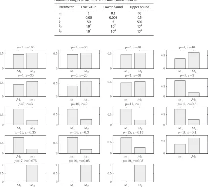
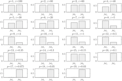
Fig. 3shows the model posterior probabilities over the different populations and the associated tolerance threshold. One observes that at high tolerance thresholdsð

e

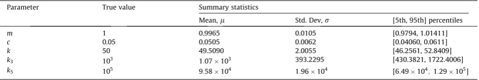
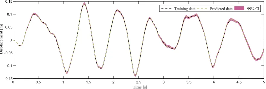
>10Þ, there is no strong evidence for either model. Between populations 8 and 15, although the training data was generated from the cubic-quintic model, the algorithm tends to favour the simplest model (the cubic model). In other words, the algorithm tries at first to converge towards the most simple model. This means that the complex model with higher number of parameters is implicitly penalised. For instance, this is quite obvious at popula-tion 14, where the probability associated to the cubic model is equal to 0.797 against 0.203 for the cubic-quintc model. How-ever, by further decreasing the tolerance threshold, it seems that the cubic model is no longer able to guarantee model prediction with sufficiently good accuracy, and for that reason, the algorithm jumps to the complex model to better accom-modate the nonlinearity coming from the quintic term and satisfy the requested accuracy. At population 16ð

e

¼0_:1Þ, the algorithm gives a higher evidence to the cubic-quintic model. The algorithm ends up by finding the true model at population 17 with strong evidence where the cubic model is eliminated, since at that level of precision, the model is no longer able to explain the data. In the subsequent iterations the algorithm refines the model parameter estimates associated to the true model.Fig. 4shows the histograms of the cubic-quintic model parameters. One may observe that these histograms are well peaked around the true values from which the training data were generated.Table 2shows the statistics related to the cubic-quintic model estimated from the last population. The results are excellent because the true values are within the (5th, 95th) percentiles. Using the mean value estimates from the last population, the prediction can now be made.Fig. 5shows the train-ing data and the model prediction with the 99% confidence interval. One observes a good agreement between the observed and predicted data where the MSE is equal to 0.0101. It should be noted that the 99% confidence interval is estimated from

0 0.5 1 1.5 2 2.5 3 3.5 4 4.5 5

Time [s] -40

-20 0 20 40

Force [N]

(6)

the obtained posterior distribution of model parameters. One way to do this is to generate randomly a large number of sam-ples, simulate the model responses and then the 99% confidence interval is found pointwise.

One may observe fromFig. 6, how the extent of model parameters evolves over populations. It is clear how by gradually decreasing the tolerance thresholds, the algorithm moves towards the true parameter values. After a few iterations, the uncertainties related to the unknown parameters start to stabilise and the algorithm converges.

Fig. 3.Posterior probabilities for the cubic and cubic-quintic models.

0 0.5 1 1.5 2 2.5 3 3.5 4 4.5 5

Time [s] -0.2

-0.1 0 0.1 0.2

[image:6.544.115.427.56.159.2]

Displacement [m]

[image:6.544.57.483.209.591.2]

Fig. 2.Training data from the cubic-quintic model (free-of-noise).

Table 1

Parameter ranges of the cubic and cubic-quintic models.

Parameter True value Lower bound Upper bound

m 1 0.1 10

c 0.05 0.005 0.5

k 50 5 500

k3 103 ₁₀2 ₁₀4

(7)

As one may notice earlier fromFig. 3, based on the training data generated from the cubic-quintic model, it was very dif-ficult to favour one model at the beginning of the algorithm. This means that both models could potentially explain the data. To better examine the prediction capability of the cubic model, one assumes that the target tolerance is equal to 0.15 (pop-ulation 15). Based on the mean parameter values obtained from that pop(pop-ulation, one may now predict the response.Fig. 7

0.96 0.98 1 1.02 1.04

m

0 100 200

Frequency

0.03 0.04 0.05 0.06 0.07

c

0 100 200

Frequency

40 45 50 55

k

0 100 200

Frequency

0 500 1000 1500 2000

k 3 0

100 200

Frequency

0 5 10 15

k

5 ×10

4

0 100 200

[image:7.544.122.430.53.281.2]

Frequency

Fig. 4.Histograms of the cubic-quintic model parameters (the red triangles show the parameter values used to generate the training data). (For

[image:7.544.43.509.348.426.2]

interpretation of the references to colour in this figure legend, the reader is referred to the web version of this article.)

Table 2

Parameter estimates for the cubic-quintic model.

Parameter True value Summary statistics

Mean,l Std. Dev,r [5th, 95th] percentiles

m 1 0.9965 0.0105 [0.9794, 1.01411]

c 0.05 0.0505 0.0062 [0.04060, 0.0611]

k 50 49.5090 2.0055 [46.2561, 52.8409]

k3 103 ₁_:₀₇₁₀3 _393.2295 _{[430.3821, 1722.4006]}

k5 105 ₉_:₅₈₁₀4 ₁_:₉₆₁₀4 _[6_:₄₉₁₀4_;₁_:₂₉₁₀5_]

0 0.5 1 1.5 2 2.5 3 3.5 4 4.5 5

Time [s]

-0.15 -0.1 -0.05 0 0.05 0.1 0.15

Displacement [m]

Training data Predicted data 99% CI

[image:7.544.76.476.380.602.2]

(8)

shows that even the cubic model provides acceptable prediction. The estimated parameters used to predict the response are summarised inTable 3. As one may observe, the nonlinear stiffness parameter in the cubic model is overestimated to com-pensate for the nonlinearity coming from the quintic term. The cubic model fits the training data with accuracy MSE = 0.0946 while the cubic-quintic model exhibits the better MSE = 0.0101.

8 10 12 14 16 18 20

Population number 0.8

0.9 1 1.1 1.2 1.3 1.4

m

True value Mean value (±2σ)

8 10 12 14 16 18 20

Population number 0.05

0.1 0.15 0.2

c

8 10 12 14 16 18 20

Population number 20

30 40 50 60 70 80

k

8 10 12 14 16 18 20

Population number 0

1000 2000 3000 4000 5000

k3

8 10 12 14 16 18 20

Population number 0

1 2 3 4 5

k 5 ×105

[image:8.544.52.491.54.395.2]

Fig. 6.Evolution of mean, upper and lower 2rvalues of the cubic-quintic model parameters over the last populations with the true value also shown

(dashed line).

0 0.5 1 1.5 2 2.5 3 3.5 4 4.5 5

Time [s]

-0.15 -0.1 -0.05 0 0.05 0.1 0.15

Displacement [m]

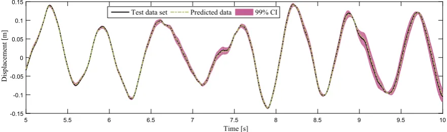
[image:8.544.50.490.444.591.2]

(9)

To investigate the validity of the selected model against new data, an independent data set of length 500 is synthetically generated.Fig. 8shows the model prediction and the 99% credibility interval where one observes that the model performs perfectly well. An estimation of the MSE gives a value of 0.0171.

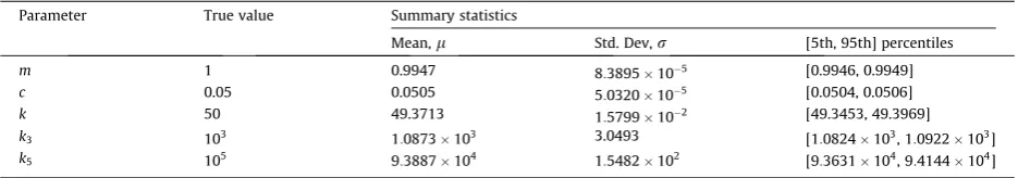
One important point should be highlighted in this example is the uncertainty on the cubic and quintic stiffness coeffi-cients. FromTable 2, one can see that those parameters have been inferred with large uncertainty. This is related to the selected target tolerance threshold value which is equal to 0.03 to keep the computational time reasonable. It should be noted that in the ABC algorithm in general, one usually aims to strike the right balance between the computational time and the precision on the posterior estimates. To reduce the uncertainty on the posterior estimates, one can further decrease the target tolerance threshold value to 9:4103.Table 4summarises the posterior estimates from where one can see that the uncertainty on the posterior estimates has been considerably reduced. Obviously, the decrease in the target tolerance threshold value automatically increases the computational time.

[image:9.544.44.506.70.323.2]

In the following, one considers noisy excitation to investigate how this may impact the model selection issue. A Gaussian noise with zero mean and 5 per cent standard deviation is added to the base excitation. The same hyperparameters defined previously are used for the ABC-SMC implementation.Fig. 9shows the model posterior probabilities over the populations. At the beginning of the algorithm, the plausibilities of the competing models are almost the same until iteration 7, then there is some evidence to suggest that the correct model is the cubic one (for instance at population 14, the posterior probability of the cubic model is 0.811 against 0.189 for the cubic-quintic). Then, at population 15ð

e

¼0_:15Þthe algorithm assigns nearly the same plausibility to both models before converging to the true model at population 16.Fig. 10depicts the model pre-diction using the mean values estimated from the last population and the 99% confidence interval. Here the MSE = 0.0256.Table 5summarises the statistics related to the model parameters. The obtained results are excellent, since

Table 3

Parameter estimates for the cubic model, (population 15,e¼0:15).

m 1 0.9589 0.0166 [0.9307, 0.9848]

c 0.05 0.0306 0.0106 [0.0134, 0.047943]

k 50 39.6658 1.5462 [37.0629, 42.2462]

k3 103 2:996103 238.6501 [2:5929103, 3:3896103]

5 5.5 6 6.5 7 7.5 8 8.5 9 9.5 10 Time [s]

-0.15 -0.1 -0.05 0 0.05 0.1

Displacement [m]

Test data set Predicted data 99% CI

[image:9.544.41.509.608.690.2]

Fig. 8.Cubic-quintic model prediction using test data set.

Table 4

Parameter estimates for the cubic-quintic model with reduced uncertaintyðe¼9:4103 ).

m 1 0.9947 ₈_:₃₈₉₅105 [0.9946, 0.9949]

c 0.05 0.0505 5:0320105 [0.0504, 0.0506]

k 50 49.3713 ₁_:₅₇₉₉102 [49.3453, 49.3969]

k3 103 ₁_:₀₈₇₃₁₀3 _3.0493 _[1_:₀₈₂₄₁₀3_{, 1}_:₀₉₂₂₁₀3_]

(10)

[image:10.544.58.484.54.335.2]

Fig. 9.Posterior probabilities for the cubic and cubic-quintic models using noisy excitation.

0 0.5 1 1.5 2 2.5 3 3.5 4 4.5 5

Time [s]

-0.15 -0.1 -0.05 0 0.05 0.1 0.15

Displacement [m]

[image:10.544.50.489.384.515.2]

Fig. 10.Cubic-quintic model prediction using noisy excitation.

Table 5

Parameter estimates related to the cubic-quintic model under noisy excitation.

m 1 1.0033 0.01579 [0.9782, 1.0293]

c 0.05 0.04684 0.0097 [0.03095, 0.0629]

k 50 49.7935 2.5377 [45.49519, 53.84228]

k3 103 ₁_:₀₂₅₁₀3 _491.9020 _{[241.0759, 1826.4790]}

[image:10.544.36.506.579.654.2]

(11)

the true values are within the (5th, 95th) percentiles. From the same table, one can see that the cubic and quintic stiffness coefficients have been inferred with large uncertainty. As mentioned before the uncertainty on the stiffness coefficients could be more reduced by further decreasing the target tolerance threshold value.

So far, the main conclusion derived from the first example is the ability of the ABC-SMC to converge efficiently towards the true model from which the training data was generated even in the presence of noise in either the system response or the input excitation. One important feature which can be noticed is that at the beginning of the Bayesian inference, the algorithm favours simpler models which is consistent with the Bayesian philosophy and the parsimony principle. In other words, the algorithm penalises implicitly complex models. This point is fundamental in Bayesian inference to avoid overfitting issues and then to guarantee a better generalisation capability with the selected model. It is clear from this example that the ABC-SMC approach automatically enforces model parsimony without the need of any other information criteria to be evaluated.

[image:11.544.52.493.541.672.2]

As before, one can now evaluate the predictive performance of the selected model using an independent test data set. Fig. 11shows the model prediction and the 99% credibility bounds where one can see that the model performs quite well. The MSE estimated on the test data set is equal to 0.0671.

3.2. Example 2: identification of a Bouc-Wen model

The identification of the Bouc-Wen (BW) model has been widely investigated in the literature by various different meth-ods[33]. The highly nonlinear nature of the BW model, along with a large number of model parameters, has made the iden-tification of this system a challenging task. The model has been receiving more attention in recent times due to the development of efficient numerical algorithms that can be used to identify the model parameters more accurately. Several methods have been discussed in the literature to accomplish this, including Levenberg-Marquardt[34], reduced gradient methods[35], and extended Kalman filters[36]. Due to the nonlinear nature of the problem, stochastic optimisation algo-rithms have been also found to be well suited. Algoalgo-rithms such as genetic algoalgo-rithms[37,38], particle swarm optimisation [39], and differential evolution[40]have been successfully implemented. However, optimisation algorithms provide a single optimum value, while the Bayesian inference allows users to get the full parameter distribution, yielding more important information.

3.2.1. Equations of motion

The general single-degree-of-freedom (SDOF) hysteretic system described in the terms of Wen[41], is represented below, wheregðy;y_Þis the polynomial part of the restoring force,zðy;y_Þis the hysteretic part andfðtÞis the excitation force:

my€þgðy;y_Þ þzðy;y_Þ ¼fðtÞ ð8Þ

where,mis the mass, and the polynomial part of the restoring force is assumed to be linear given by the following equation:

gðy;y_Þ ¼cy_þky ð9Þ

The hysteretic component is defined by Wen[41]via the additional equation of motion:

_

z¼

a

jy_jznby_jznj þAy_; fornodd

_a

jy_jzn1_j_z_j_b_y_{_}_j_zn_{j þ}_A_y_{_}_; _for_n_even

ð10Þ

The parameters

a

; bandngovern the shape and the smoothness of the hysteresis loop. It should be noted that the equations offer a simplification from the point of view of parameter estimation, in that the stiffness term in Eq.(9)can be combined with theAy_ term in the state equation forz. The reader can refer to[42]for full details.

In this example, the response output will be assumed to be displacement. The sampling interval was taken as 0.001 s, corresponding to a sampling frequency of 1000 Hz. Here, as in the first example, the excitation is Gaussian with zero mean

5 5.5 6 6.5 7 7.5 8 8.5 9 9.5 10 Time [s]

-0.15 -0.1 -0.05 0 0.05 0.1 0.15

Displacement [m]

(12)

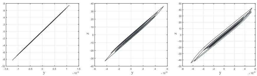
and standard deviation of 10. The exact parameter values used to generate the training data and the parameter ranges are summarised inTable 6.Fig. 12shows the BW model response withn¼2. The training data used here were composed of 1000 points corresponding to a record duration of 1 s.Fig. 13shows (from left to right) the hysteresis loops obtained for three different standard deviation values of the excitation equal to 10, 30 and 40.

To identify the BW model parameters, one converts the problem of parameter identification into a model selection prob-lem for design purposes. One can illustrate the model selection probprob-lem by proposing a range of potential models: first a simple linear model is considered. Then, more complex models are defined by varyingnin the equations of motion from 1 to 4. In total, five competing models are considered denoted by:

M1 : m€yþcy_þAy¼fðtÞ ð11Þ

M2:5 : Eqs:ð8Þandð10Þ; n¼1:4 ð12Þ

To implement the ABC-SMC algorithm, equal prior probabilities PrðMi¼1:5Þ ¼15are considered. In this example, the

toler-ance threshold sequence is adaptively defined. It has been found after a few tests that a tolertoler-ance threshold set at the 20th percentile of the particle distances from the previous iteration maintains a quite satisfactory acceptance rate through the populations. The rest of the hyperparameters are selected as in the first example. The stopping criterion chosen here is when the difference between two consecutive tolerance thresholds is less than or equal to 5104_{. The obtained results are}

[image:12.544.167.373.73.135.2]

sum-marised below using noisy measurements; noise of RMS 1% was added to the displacement signal.

Table 6

Parameter ranges of the Bouc-Wen model.

Parameter True value Lower bound Upper bound

m 1 0.1 10

c 20 2 200

a 1.5 0.15 15

b 1.5 15 0.15

A 6680 668 66800

0 0.1 0.2 0.3 0.4 0.5 0.6 0.7 0.8 0.9 1

Time [s] -2

-1 0 1 2

Displacement [m]

×10-3

[image:12.544.72.473.164.290.2]

Training data

Fig. 12.Training data from the Bouc-Wen model.

-1.5 -1 -0.5 0 0.5 1 1.5

y ×10-3

-10 -8 -6 -4 -2 0 2 4 6 8

z

-6 -4 -2 0 2 4 6

y ×10-3

-40 -30 -20 -10 0 10 20 30 40

z

-8 -6 -4 -2 0 2 4 6

y ×10-3

-50 -40 -30 -20 -10 0 10 20 30 40 50

[image:12.544.54.491.332.461.2]

z

(13)

[image:13.544.59.491.52.363.2]

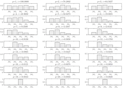
Fig. 14.Model posterior probabilities of the Bouc-Wen model over the populations.

0.99 0.995 1 1.005 m

0 100 200

Frequency

19.85 19.9 19.95 20 20.05 c

0 100 200

Frequency

1.5 1.55 1.6 1.65 1.7

α

0 100 200

Frequency

-2.5 -2 -1.5 -1 -0.5

β

0 100 200

Frequency

6620 6640 6660 6680 6700 6720 A

0 100 200

Frequency

Fig. 15.Histograms of the identified Bouc-Wen model parameters (the red triangles show the true values). (For interpretation of the references to colour in

[image:13.544.119.430.410.631.2]

(14)

Fig. 14shows how ABC-SMC eliminates the least likely models progressively. One may observe thatM5is the first one to

be eliminated which means that it is inadequate to explain the data. Next, the linear model is eliminated one population after. The modelsM2!4seem the most likely candidates to explain the data since after eliminatingM5andM1, it seems

quite difficult to favour one model over another. One may observe fromFig. 14that only at population 18ð

_e

¼0:0058Þ, does the algorithm start to favourM3. This would suggest that evenM2andM4may explain the data reasonably well with a

preference for M3. The algorithm identifies with an obvious evidence, the true model at population 19 ð

e

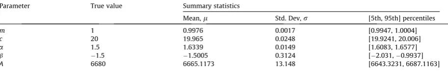
¼0:0042Þ.

Fig. 15shows the histograms of the model parameter values, in which one can see a visible bias on all the parameter esti-mates exceptbbecause of the noise in the training data. From the last population, one may estimate the parameter statistics related to the selected model (see,Table 7). The training data and the model prediction with the 99% confidence interval are shown inFig. 16from where one can see a sufficient accuracy. The estimation of the MSE gives a value equal to 0.0024.

Once again, the ABC-SMC algorithm is shown to be efficient in problems with a relatively large number of competing models and more importantly when those competing models are quite similar. As one may observe fromFig. 14,M2and M4 are simultaneously eliminated at population 18 with closer posterior probabilities (0.182 forM2 against 0.174 for M4). To further investigate which model is more plausible in order to provide a rational rank and to gain confidence in model

posterior probabilities, a number of simulations are carried out (20 in this case).Fig. 17shows the box-plots of the posterior model probabilities over a few populations. Clearly, the posterior model probabilities are quite repeatable with acceptable variation levels. One may observe that overall, the variations of the posterior model probabilities decrease over the popula-tions. Finally, the simulations show thatM2is more plausible thanM4which validates the results obtained from a single

simulation.

Once the model is selected and its parameters are estimated, it can now be used to make predictions on new unseen data. To do so, a test data set of length 1000 is synthetically generated.Fig. 18shows the model prediction with the 99% credibility interval. The result shows a good agreement between the test data set and the model prediction. An estimation of the MSE gives a value of 0.007.

[image:14.544.46.503.74.147.2]

Based on the examples presented so far, it is clear that ABC-SMC deals well with model selection and parameter estima-tion. In the first two examples, the MSE based on the time series has been used to measure the similarity between the observed and simulated data. The next example, will investigate in more detail, the flexibility of ABC-SMC to infer system

Table 7

Bouc-Wen model parameter estimates from the last population.

m 1 0.9976 0.0017 [0.9947, 1.0004]

c 20 19.965 0.0248 [19.9241, 20.006]

a 1.5 1.6339 0.0149 [1.6083, 1.6577]

b 1.5 1.5005 0.3124 [2.031,0.9937]

A 6680 6665.1173 13.148 [6643.3231, 6687.1163]

0 0.1 0.2 0.3 0.4 0.5 0.6 0.7 0.8 0.9 1

Time [s]

-2 -1.5 -1 -0.5 0 0.5 1 1.5 2

Displacement [m]

×10-3

[image:14.544.42.492.103.372.2]

(15)

models by using other features and through different metrics to measure the similarity between observed and simulated data.

3.3. Example 3: Duffing oscillator

The final example is about the identification of a Duffing oscillator without linear stiffness. In this case, the system may bifurcate and show a high sensitivity to small variations that may affect the parameters. Through this example, we aim to

M1 M2 M3 M4 M5 0.16

0.18 0.2 0.22 0.24 0.26

Posterior probabilities

p=1,ε=100.0000

M1 M2 M3 M4 M5 0

0.05 0.1 0.15 0.2 0.25 0.3 0.35

p=5,ε=33.4787

M1 M2 M3 M4 M5 0

0.1 0.2 0.3 0.4

p=8,ε=4.8075

M1 M2 M3 M4 M5 0

0.1 0.2 0.3 0.4 0.5 0.6

p=13,ε=0.1095

M1 M2 M3 M4 M5 0

0.1 0.2 0.3 0.4 0.5

p=15,ε=0.0254

M1 M2 M3 M4 M5 0

0.1 0.2 0.3 0.4

p=16,ε=0.0144

M1 M2 M3 M4 M5 0

0.1 0.2 0.3 0.4 0.5 0.6

p=18,ε=0.0063

M1 M2 M3 M4 M5 0

0.2 0.4 0.6 0.8 1

[image:15.544.53.495.50.591.2]

p=19,ε=0.0048

(16)

1 1.1 1.2 1.3 1.4 1.5 1.6 1.7 1.8 1.9 2 Time [s]

-1.5 -1 -0.5 0 0.5 1 1.5 2

Displacement [m]

×10-3

[image:16.544.47.488.59.226.2]

Fig. 18.Bouc-Wen model prediction using test data set.

0 5 10 15 20 25 30 35 40 45 50 Time [s]

-5 0 5

Displacement [m]

[image:16.544.51.488.264.386.2]

True parameters Perturbed parameters

[image:16.544.37.507.445.479.2]

Fig. 19.Comparison between the Duffing oscillator responses using the true and perturbed parameters.

Table 8

True and perturbed parameters used for the Duffing oscillator.

m c k3 MSE

True parameters 1 0.05 1

Perturbed parameters 0.999 0.0489 1.005 32.1707

-150 -100 -50 0 50 100 150

Acceleration (m/s2) 10-7

10-6 10-5

10-4 10-3 10-2

10-1

[image:16.544.169.372.507.672.2]

Log(PDF) True parameters_{Perturbed parameters}

(17)

investigate the potential of the ABC-SMC algorithm to deal with such complex scenarios by choosing a suitable feature and a corresponding metric to make inference possible. The Duffing oscillator considered here is given by Eq.(13):

my€þcy_þk3y3¼fðtÞ ð13Þ

wheremis the mass,cis the damping coefficient andk3is the nonlinear stiffness,fðtÞis a Gaussian input force.

Fig. 19shows the displacement output of the Duffing oscillator using the true and perturbed set of parameters shown in Table 8. It should be noted that the perturbed values were obtained from the system output using the restoring force surface method[43]. One observes a clear divergence (the grey band inFig. 19) which means that the perturbed parameters that could be a potential solution for the system would be rejected. This is a typical example where the classical Bayesian infer-ence based on the time-series data and a Gaussian likelihood function cannot perform well. Here, it is demonstrated how ABC-SMC can deal with such a challenging situation and infer the model by selecting a suitable feature and a corresponding metric to measure the level of agreement between observed and simulated data.

In this illustrative example, it was found that the probability density function (PDF) of the acceleration is insensitive to small changes and thus can be used as a main feature to make inference.Fig. 20depicts the PDFs of the acceleration using initial and perturbed sets of parameters. It is clear that the acceleration PDF is a promising feature since it remains nearly invariant when input parameters are subjected to small changes. As one may see from the same figure, the variation is mainly visible on the tails of the distributions which gives small impact on the metric value. This means that the PDF of the acceleration might serve as a robust feature to infer the Duffing oscillator. The Euclidean distance between the observed and simulated PDFs, given by Eq.(14), is used to measure the degree of agreement. Of course, the inference can be carried out using other kinds of features, for instance, it was shown in[44]that the spectrum is also insensitive to small parameter vari-ations, which means that it can be used as a basis for comparison. In the same way, various metrics such as the Kullback-Leibler divergence[45]or the maximum mean discrepancy[46]for instance, can be used to measure the similarity/dissim-ilarity between two PDFs.

D

ðpl

f;^p l fÞ ¼

Xn

l¼1 logðpl

fÞ logðp^flÞ

2

" #1

2

ð14Þ

wherepl

f and^plf are the probabilities associated with the observed and simulated data, respectively.

In the final example, model selection is again pursued to infer the Duffing oscillator model (denoted here byM2). This is

illustrated by considering the linear model (denoted here byM1) as another potential candidate. For ABC-SMC

[image:17.544.61.490.53.335.2]

implemen-tation, one keeps the same hyperparameters with a total number of iterations set to 25. As in the previous examples, the

(18)

[image:18.544.54.494.57.416.2]

acceleration was corrupted by noise, a 1% RMS of the response is added to the signal.Fig. 21shows the model posterior prob-abilities over the populations. After a few populations, the algorithm converges to the correct model as expected, precisely at population 6. From population 7 to population 25 the algorithm refines the model parameter estimates.

Fig. 22shows in the logarithmic scale the PDF of the true response and the predicted ones obtained from Monte Carlo simulations (MCS) (1000 realisations) over a few populations. One observes how by decreasing gradually the tolerance schedule value, one gains confidence in the prediction.

-300 -200 -100 0 100 200 300

Acceleration (m/s2)

10-7 10-6 10-5 10-4 10-3 10-2 10-1 Log(PDF)

p=6,ε=1.2032

True response Predicted responses

-150 -100 -50 0 50 100 150

Acceleration (m/s2)

10-7 10-6 10-5 10-4 10-3 10-2 10-1 Log(PDF)

p=13,ε=0.25869

-150 -100 -50 0 50 100 150

Acceleration (m/s2₎ 10-7 10-6 10-5 10-4 10-3 10-2 10-1 Log(PDF)

p=18,ε=0.069012

-150 -100 -50 0 50 100 150

Acceleration (m/s2₎ 10-7 10-6 10-5 10-4 10-3 10-2 10-1 Log(PDF)

p=25,ε=0.0068333

Fig. 22.True and predicted PDFs of the acceleration using MCS for the Duffing oscillator.

0.9992 0.9994 0.9996 0.9998 1 1.0002 1.0004 1.0006 1.0008

m 0 20 40 60 80 100 120 140 160 180 Frequency

0.04985 0.0499 0.04995 0.05 0.05005 0.0501 0.05015

c 0 20 40 60 80 100 120 140 160 Frequency

0.996 0.997 0.998 0.999 1 1.001 1.002 1.003 1.004

[image:18.544.54.490.456.562.2]

k3 0 20 40 60 80 100 120 140 160 180 Frequency

Fig. 23.Histograms of the Duffing oscillator parameters (the red triangles show the true values). (For interpretation of the references to colour in this figure

(19)

Fig. 23shows the histograms of the Duffing oscillator parameters. One may observe that the obtained histograms are well peaked in the true values.Fig. 24shows the observed and predicted PDFs of the acceleration in the logarithmic scale, in which a good agreement is shown (the 99% confidence interval is not shown here as it is indistinguishable from the plotted responses). This example shows that the PDF of the acceleration can be used as a robust feature to infer the Duffing oscillator model. One can see fromTable 9that the original parameters are accurately estimated.

In short, this example demonstrates that the acceleration PDF remains invariant when the Duffing oscillator undergoes small changes in parameters. Thus, the acceleration PDF can be used as a feature to perform model selection and parameter estimation in a Bayesian framework, unlike the time-series error. Despite its simplicity, this example shows many interest-ing and promisinterest-ing aspects of the ABC-SMC algorithm to deal efficiently with model selection and parameter estimation by introducing new features as a basis for comparison to infer complex system models.

4. Conclusion

Through different illustrative examples, it has been demonstrated that the ABC-SMC algorithm is an excellent way to deal with model selection and parameter estimation issues with some advantages over traditional Bayesian methods in the speci-fic circumstances described in this paper. The ABC-SMC algorithm has several very useful properties: (i) ease of implemen-tation, (ii) generality of application and (iii) the ability to deal with model selection for larger numbers of models in a straightforward way. The flexibility offered by ABC-SMC can be useful to infer systems with complex behaviours using dif-ferent kinds of features for systems with larger datasets, from which one may extract useful summary statistics.

In conclusion, the algorithm was capable of estimating the parameters of three different dynamical systems efficiently by using different kinds of features and metrics. Hence, ABC-SMC offers a new possibility for model selection and parameter estimation for dynamical systems in an efficient way. Scope for future work is vast, including the replacement of the sim-ulation by a surrogate model to reduce the computational requirements and speed up the algorithm for more challenging situations. In addition, the development of ‘‘good” features, insensitive to small variations to deal with model selection and parameter estimation efficiently, can be used in a more challenging context, such as model validation. Finally, we hope that the present paper will fuel further studies in the structural dynamics community on more realistic case studies.

Acknowledgements

[image:19.544.170.378.56.222.2]

The support of the UK Engineering and Physical Sciences Research Council (EPSRC) through grant reference No. EP/ K003836/1 is greatly acknowledged.

Table 9

Model parameter estimates of the Duffing oscillator.

m 1 1.0000 0.0003 [0.9995, 1.0005]

c 0.05 0.0500 0.0001 [0.0499, 0.0501]

k3 1 1.0001 0.0015 [0.9976, 1.0025]

-150 -100 -50 0 50 100 150

Acceleration (m/s2)

10-7 10-6 10-5 10-4 10-3 10-2 10-1

Log(PDF) True response

Predicted response

[image:19.544.43.509.282.340.2]

(20)

References

[1]M. Muto, J.L. Beck, Bayesian updating and model class selection for hysteretic structural models using stochastic simulation, J. Vib. Control. 14 (1–2)

(2008) 7–34.

[2]B.A. Zárate, J.M. Caicedo, J. Yu, P. Ziehl, Bayesian model updating and prognosis of fatigue crack growth, Eng. Struct. 45 (2012) 53–61.

[3]Ph. Bisaillon, R. Sandhu, M. Khalil, C. Pettit, D. Poirel, A. Sarkar, Bayesian parameter estimation and model selection for strongly nonlinear dynamical

systems, Nonlinear Dyn. 82 (2015) 1061–1080.

[4]J.L. Beck, K.V. Yuen, Model selection using response measurements: Bayesian probabilistic approach, J. Eng. Mech. 130 (2) (2004) 192–203.

[5]R. Sandhu, M. Khalil, A. Sarkara, D. Poirelc, Bayesian model selection for nonlinear aeroelastic systems using wind-tunnel data, Comput. Methods Appl.

Mech. Eng. 282 (2014) 161–183.

[6]T.G. Ritto, L.C.S. Nunes, Bayesian model selection of hyperelastic models for simple and pure shear at large deformations, Comput Struct. 156 (2015)

101–109.

[7]P.J. Green, Reversible jump Markov chain Monte Carlo computation and Bayesian model determination, Biometrika 82 (4) (1995) 711–732.

[8]R.E. Kass, A.E. Raftery, Bayes factors, J. Am. Stat. Assoc. 90 (1995) 773–795.

[9] DB. Rubin, Using the SIR algorithm to simulate posterior distributions, in: Proceedings of the Third Valencia International Meeting, 1987, Bayesian Statistics (3), 1989, pp. 395–402.

[10] F. Cadini, C. Sbarufatti, M. Corbetta, M. Giglio, A particle filter-based model selection algorithm for fatigue damage identification on aeronautical

structures, Struct. Control Health Monit. (2017) e2002.

[11]H. Akaike, Information theory and an extension of the maximum likelihood principle, Breakthroughs in Statistics, vol. I, Springer, 1992, pp. 610–624.

[12]G. Schwarz, Estimating the dimension of a model, Ann. Stat. 6 (2) (1978) 461–464.

[13]A.A. Neath, J.E. Cavanaugh, The Bayesian information criterion: background, derivation, and applications, Wiley Interdiscip. Rev. Comput. Stat. 4 (2)

(2012) 199–203.

[14]C.A. McGrory, D.M. Titterington, Variational approximations in Bayesian model selection for finite mixture distributions, Comput. Stat. Data Anal. 51

(2007) 5352–5367.

[15]J. Skilling, Nested sampling, in: R. Fischer, R. Preuss, U.V. Toussaint (Eds.), American Institute of Physics Conference Series, 2004, pp. 395–405.

[16]J. Skilling, Nested sampling for general Bayesian computation, Bayesian Anal. 1 (4) (2006) 833–860.

[17]L. Mthembu, T. Marwala, M. Friswell, S. Adhikari, Model selection in finite element model updating using the Bayesian evidence statistic, Mech. Syst.

Signal. Process. 25 (2011) 2399–2412.

[18]AH. Elsheikh, I. Hoteit, M.F. Wheeler, Efficient Bayesian inference of subsurface flow models using nested sampling and sparse polynomial chaos

surrogates, Comput. Methods Appl. Mech. Eng. 269 (2014) 515–537.

[19]M. Beaumont, J. Cornuet, J. Marin, C. Robert, Adaptive approximate Bayesian computation, Biometrika 96 (4) (2009) 983–990.

[20] T. Toni, M.P.H. Stumpf, Simulation-based model selection for dynamical systems in systems and population biology, Bioinformatics 26 (1) (2010) 104–

110.

[21]Ch. Barnes, D. Silk, M.P.H. Stumpf, Bayesian design strategies for synthetic biology, Interface Focus 1 (2011) 895–908.

[22]B.M. Turner, T. Van Zandt, A tutorial on approximate Bayesian computation, J. Math. Psychol. 56 (2012) 69–85.

[23] A. Ben Abdessalem, N. Dervilis, D. Wagg, K. Worden, Identification of nonlinear dynamical systems using approximate Bayesian computation based on a sequential Monte Carlo sampler, in: International Conference on Noise and Vibration Engineering, September 19–21, 2016, Leuven, Belgium.

[24]M. Chiachio, J.L. Beck, J. Chiachio, G. Rus, Approximate Bayesian computation by Subset Simulation, SIAM J. Sci. Comput. 36 (3) (2014) A1339–A1358.

[25]S.K. Au, J.L. Beck, Estimation of small failure probabilities in high dimensions by subset simulation, Probab. Eng. Mech. 16 (2001) 263–277.

[26]P. Marjoram, J. Molitor, V. Plagnol, S. Tavare, Markov chain Monte Carlo without likelihoods, Proc. Natl. Acad. Sci. USA 100 (2003) 15324–15328.

[27]T. Toni, D. Welch, N. Strelkowa, A. Ipsen, M.P.H. Stumpf, Approximate Bayesian computation scheme for parameter inference and model selection in

dynamical systems, J. Roy. Soc. Interface 6 (2009) 187–202.

[28]J. Ching, J.L. Beck, K. Porter, Bayesian state and parameter estimation of uncertain dynamical systems, Probab. Eng. Mech. 21 (2006) 81–96.

[29] A. Doucet, On sequential Monte Carlo methods for Bayesian filtering, Dept. Eng., Univ. Cambridge, UK, Tech. Rep., 1998.

[30] A. Doucet, S. Godsill, C. Andrieu, On sequential Monte Carlo sampling methods for Bayesian filtering, Statist. Comput. 10 (3) (2000) 197–208.

[31] A. Doucet, A.M. Johansen. A tutorial on particle filtering and smoothing: fifteen years later, technical report, 2008.

[32]S. Filippi, C.P. Barnes, J. Cornebise, M.P.H. Stumpf, On optimality of kernels for approximate Bayesian computation using sequential Monte Carlo, Stat.

Appl. Genet. Mol. Biol. 12 (2013) 87–107.

[33]J.P. Noël, G. Kerschen, Nonlinear system identification in structural dynamics: 10 more years of progress, Mech. Syst. Signal. Process. 83 (2017) 2–35.

[34]Y.Q. Ni, J.M. Ko, C.W. Wong, Identification of non-linear hysteretic isolators from periodic vibration tests, J. Sound Vib. 217 (4) (1998) 737–756.

[35]H. Zhang, G.C. Foliente, Y. Yang, F. Ma, Parameter identification of inelastic structures under dynamic loads, Earthq. Eng. Struct. Dyn. 31 (2002) 1113–

1130.

[36]J.S. Lin, Y. Zhang, Nonlinear structural identification using extended Kalman filter, Comput. Struct. 52 (4) (1994) 757–764.

[37]B.P. Deacon, K. Worden, Identification of hysteretic systems using genetic algorithms, in: Proceedings of EUROMECH-2nd European Nonlinear

Oscillations Conference, Prague, 1996, pp. 55–58.

[38]K. Chwastek, J. Szczyglowski, Identification of a hysteresis model parameters with genetic algorithms, Math. Comput. Simul. 71 (2006) 206–211.

[39]S. Xiao, Yangmin Li, Dynamic compensation andH1control for piezoelectric actuators based on the inverse Bouc-Wen model, Robot. Cim. Int. Manuf.

30 (2014) 47–54.

[40] A. Kyprianou, K. Worden, Identification of hysteretic systems using the differential evolution algorithm, J. Sound Vib. 248 (2) (2001) 289–314.

[41]Y. Wen, Method for random vibration of hysteretic systems, ASCE J. Eng. Mech. Division 102 (2) (1976) 249–263.

[42]K. Worden, J.J. Hensman, Parameter estimation and model selection for a class of hysteretic systems using Bayesian inference, Mech. Syst. Signal.

Process. 32 (2012) 153–169.

[43]K. Worden, Data processing and experiment design for the restoring force surface method. Part II: Choice of excitation signal, Mech. Syst. Signal.

Process. 4 (1990) 321–344.

[44]K. Worden, Some thoughts on model validation for nonlinear systems, in: IMAC-XIX,19th_{International Modal Analysis Conference in Orlando, Florida,}

2001.

[45]S. Kullback, Information Theory and Statistics, Dover Publications Inc., Mineola, New York, 1968.

[46]A. Gretton, K.M. Borgwardt, M. Rasch, B. Schölkopf, A.J. Smola, A Kernel approach to comparing distributions, Proceedings of the Twenty-Second AAAI