On the Cause of Recent Variations in Lower Stratospheric Ozone

(1)

On the Cause of Recent Variations in Lower

Stratospheric Ozone

Martyn P. Chipperﬁeld1,2 , Sandip Dhomse1 , Ryan Hossaini3 , Wuhu Feng1,4 , Michelle L. Santee5 , Mark Weber6 , John P. Burrows6 , Jeanette D. Wild7,8 , Diego Loyola9 , and Melanie Coldewey-Egbers9

1

School of Earth and Environment, University of Leeds, Leeds, UK,2National Centre for Earth Observation, University of Leeds, Leeds, UK,3_{Lancaster Environment Centre, Lancaster University, Lancaster, UK,}4_{National Centre for Atmospheric}

Science, University of Leeds, Leeds, UK,5Jet Propulsion Laboratory, California Institute of Technology, Pasadena, CA, USA,

6_{Institute of Environmental Physics, University of Bremen, Bremen, Germany,}7_{Innovim LLC, Greenbelt, MD, USA,}8_NOAA/

NCEP/Climate Prediction Center, College Park, MD, USA,9Deutsches Zentrum für Luft-und Raumfahrt (DLR), Institut für Methodik der Fernerkundung (IMF), Oberpfaffenhofen, Germany

Abstract

We use height-resolved and total column satellite observations and 3-D chemical transport model simulations to study stratospheric ozone variations during 1998–2017 as ozone-depleting

substances decline. In 2017 extrapolar lower stratospheric ozone displayed a strong positive anomaly following much lower values in 2016. This points to large interannual variability rather than an ongoing downward trend, as reported recently by Ball et al. (2018, https://doi.org/10.5194/acp-18-1379-2018). The observed ozone variations are well captured by the chemical transport model throughout the stratosphere and are largely driven by meteorology. Model sensitivity experiments show that the contribution of past trends in short-lived chlorine species to the ozone changes is small. Similarly, the potential impact of modest trends in natural brominated short-lived species is small. These results conﬁrm the important role that atmospheric dynamics plays in controlling ozone in the extrapolar lower stratosphere on multiannual time scales and the continued importance of monitoring ozone proﬁles as the stratosphere changes.

Plain Language Summary

Emission of long-lived chlorine and bromine-containing

ozone-depleting substances has led to the depletion of the ozone layer, most notably the Antarctic ozone hole. Policy action through the Montreal Protocol has phased out the production of the major long-lived ozone-depleting substances. Consequently, stratospheric chlorine and bromine amounts are declining, and we expect the ozone layer to slowly recover. However, although the tropical lower stratosphere is not a region where large ozone loss has so-far been observed, a recent study by Ball et al. (2018) suggested that ozone there is decreasing, in disagreement with models and expectations of ozone recovery. We use updated observations and an atmospheric model to investigate these issues. First, we use an additional year of observations which show that ozone values in the lower stratosphere increased in 2017, which is a consequence of variations in atmospheric dynamics. Second, our 3-D model performs well in reproducing the observed ozone variations. Although the model is not perfect, the comparisons suggest that we do have a good understanding of the lower stratospheric ozone. Third, we quantify the role of short-lived chlorine and bromine compounds, which are not controlled by the Montreal Protocol, on the recent ozone changes. The effect is small.

1. Introduction

Depletion of the stratospheric ozone layer by chlorine and bromine species has been a major environmental issue since the early 1970s. Following controls on the production of the long-lived halocarbons which trans-port chlorine and bromine to the stratosphere, the ozone layer is expected to recover over the course of this century (WMO, 2014). Decreases in the stratospheric loading of chlorine and bromine have been observed, and there are signs of this resulting in an increase in ozone in the upper stratosphere and the Antarctic lower stratosphere (e.g., Chipperﬁeld et al., 2017; Harris et al., 2015; Solomon et al., 2016; Strahan & Douglass, 2017; Weber et al., 2018).

However, in contrast to this expectation of increasing stratospheric ozone, Ball et al. (2018) recently reported evidence for an ongoing decline in lower stratospheric ozone at extrapolar latitudes between 60°S and 60°N.

RESEARCH LETTER

10.1029/2018GL078071

Key Points:

•Observations show that lower stratospheric ozone at extrapolar latitudes increased strongly in 2017 relative to a negative anomaly in 2016

•Model simulations reproduce the observed ozone variations well, and the main driver in the lower stratosphere is atmospheric dynamics

•The contribution of an observation-based trend in short-lived chlorine species to recent lower stratospheric ozone variations is small

Supporting Information:

•Supporting Information S1

Correspondence to:

M. P. Chipperﬁeld, m.chipperﬁeld@leeds.ac.uk

Citation:

Chipperﬁeld, M. P., Dhomse, S., Hossaini, R., Feng, W., Santee, M. L., Weber, M., et al. (2018). On the cause of recent variations in lower stratospheric ozone.

Geophysical Research Letters,45, 5718–5726. https://doi.org/10.1029/ 2018GL078071

Received 26 MAR 2018 Accepted 22 MAY 2018

Accepted article online 30 MAY 2018 Published online 10 JUN 2018

(2)

They applied a dynamical linear modeling (DLM) regression approach (Ball et al., 2017) over the period 1998–2016 to several merged ozone data sets covering both total column and three separate height regions: lower, middle, and upper stratosphere. The DLM technique estimates smoothly varying nonlinear background trends without the prescription of any explanatory variable, such as effective equivalent stratospheric chlorine. Ball et al. (2018) found, with a high degree of probability, that between 60°S and 60°N lower stratospheric ozone, and the total stratospheric column, continued to decline from 1998 to 2016, which contradicts expectations of ozone recovery. Their DLM approach is not able to attribute this decrease to a speciﬁc process. However, they analyzed results from two nudged chemistry-climate models (CCMs) for the periods until 2014 and 2015, respectively, and found that they were not able to reproduce the observed lower stratospheric ozone changes. Ball et al. (2018) suggested possible reasons for the observed ongoing ozone decrease, and the models’inability to reproduce it, including additional ozone depletion from increasing halogenated very short-lived substances (VSLSs).

Very short-lived substances are source gases with atmospheric lifetimes of 6 months or less. Brominated VSLSs, such as bromoform and dibromoethane, which are emitted naturally from the oceans, are known to contribute about 5 ppt to the current stratospheric loading of inorganic bromine (WMO, 2014). Recently, there has been interest in chlorinated VSLSs (VSLS-Cl) which, in contrast, are largely of anthropo-genic origin. In particular, observations from global surface networks (Hossaini, Chipperﬁeld, Montzka, et al., 2015; Hossaini et al., 2017) and the upper troposphere (Oram et al., 2017) indicate an increase in compounds such as dichloromethane since the early 2000s. Hossaini et al. (2017) investigated the possible impact of an increase in VSLS-Cl on stratospheric ozone. They found only a modest contribution from VSLS-Cl increases observed so far to ozone depletion, which occurred in regions where chlorine is known to deplete ozone, notably the polar regions.

In this paper we use a detailed atmospheric chemical transport model (CTM) to investigate the results of Ball et al. (2018). We perform a range of experiments in order to quantify the possible effect of different processes on lower stratospheric ozone, including the role of halogenated VSLS. We compare the model results with satellite observations, which have been updated through to the end of 2017, that is, an additional year com-pared to the analysis of Ball et al. (2018).

2. TOMCAT 3-D CTM

We have performed a series of experiments with the TOMCAT 3-D CTM (Chipperﬁeld, 2006). The model contains a detailed description of stratospheric chemistry including heterogeneous reactions on sulfate aerosols and polar stratospheric clouds. The model was forced using European Centre for Medium-Range Weather Forecasts ERA-Interim winds and temperatures (Dee et al., 2011) and run with a resolution of 2.8° × 2.8° and 32 levels from the surface to ~60 km. The surface mixing ratios of long-lived source gases (e.g., CFCs, HCFCS, CH4, and N2O) were taken from WMO (2014) scenario A1. The solar cycle was included using time-varying solarﬂux data (1998–2017) from the Naval Research Laboratory solar variability model, referred to as NRLSSI2 (update of Coddington et al., 2016). Stratospheric sulfate aerosol surface density (SAD) data for 1998–2014 were obtained from ftp://iacftp.ethz.ch/pub_read/luo/CMIP6/ (Arfeuille et al., 2013; Dhomse et al., 2015). As the equivalent SAD values are not yet available for the later years, a consis-tent time series over the whole period is not possible; thus, for 2015–2017, the SAD values were repeated from 2014. Thus, our analysis will miss the impact on ozone of SAD changes due to the eruption of Calbuco in 2015.

(3)

TOMCAT has been shown to reproduce well observed levels of stratospheric Bry with this approach (Werner et al., 2017).

We performed a total of six simulations. The control run (CNTL) was spun up from 1977 and integrated until the end of 2017 including all of the processes described above. Sensitivity simulations were initialized from the control run in 1996 and also integrated until the end of 2017. Run NOCL removed the observation-based VSLS-Cl trend, while run EXBR assumed an additional VSLS-Br trend of 1 ppt over 20 years (0.05 ppt/yr). Although there is no direct evidence for such a trend in brominated VSLS, this change is within the uncertainty of the stratospheric VSLS-Br loading, and we wanted to investigate the potential for changes in this to impact ozone. Run fDYN was the same as CNTL but used annually repeating meteorology from 1996. Run fDYN_NOSC was the same as fDYN but used afixed solarflux from January 1996. Finally, run fDYN_NOSC_fAER was the same as fDYN_NOSC but also used a repeating aerosolfield from 1996.

3. Ozone Data Sets

We use three sources of data for column ozone comparisons:

1. Solar Backscatter Ultraviolet Radiometer (SBUV) National Oceanic and Atmospheric Administration (NOAA) merged ozone data release 6 (1998–2016) constructed by merging SBUV/SBUV2 total column and profile data. The SBUV(/2)-NOAA data set has recently been extended into 2017 with the addition of OMPS data from Suomi-NPP. The SBUV(/2)-only data set, and shortly the OMPS extension, can be obtained from ftp://ftp.cpc.ncep.noaa.gov/SBUV_CDR. The data set is composed of adjusted SBUV and SBUV/2 data from Nimbus 7 and NOAA 9, 11, 16, 17, 18, and 19. NOAA 16, 17, and 19 are adjusted tofit NOAA 18. NOAA 9 is adjusted tofit between the ascending and descending nodes of NOAA 11. In the 2017-extended data set, OMPS is adjusted to the SBUV/2 data from NOAA 19. Total column data are the sum of the layer profile data.

2. GOME-SCIAMACHY-GOME-2 (GSG) merged data set (1995–2017) constructed by merging total column ozone from Global Ozone Monitoring Experiment (GOME), the Scanning Imaging Absorption Spectrometer for Atmospheric Chartography (SCIAMACHY), and GOME-2A instruments retrieved with the WFDOAS algorithm (e.g., Weber et al., 2011, 2018). The SCIAMACHY and GOME-2A data were succes-sively bias corrected during overlap periods to the starting record of GOME. GSG data can be obtained from http://www.iup.uni-bremen.de/gome/wfdoas/merged/wfdoas_merged.html.

3. GOME-SCIAMACHY-OMI-GOME-2 Essential Climate Variable (GTO-ECV) data (1995–2017) from the ESA Climate Change Initiative (Coldewey-Egbers et al., 2015; Garane et al., 2018). GTO-ECV data are constructed by applying GOME-type Direct FITting algorithm to the GOME; SCIAMACHY, GOME-2A, GOME-2B, and Ozone Monitoring Instrument (OMI) observations. The GTO-ECV data can be obtained from https://atmos.eoc.dlr.de/gto-ecv.

For height-resolved comparisons we use Aura-Microwave Limb Sounder (MLS) v4.2 level 2 data (2004–2017). MLS data can be obtained from https://disc.gsfc.nasa.gov/datasets?page=1&keywords=ML2O3_004. MLS zonal monthly means are calculated by binning the proﬁles at model latitude intervals. For partial column ozone comparisons we also use the BAyeSian Integrated and Consolidated (BASIC) composite ozone time series data set (Alsing & Ball, 2017), described in Ball et al. (2017).

4. Results

4.1. Ozone Observations

(4)

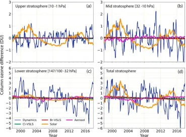
anomaly in the lower stratosphere in 2016 and consequently in the stratospheric and total column. However, the additional year of 2017 shows a strong positive anomaly of around 3 DU in the lower stratospheric and total columns. Therefore, this lengthened time series changes the appearance of a recent downward trend in lower stratospheric column ozone and suggests, rather, a more important role for atmospheric variability.

[image:4.612.220.532.91.525.2]

The results of the control model simulation in Figure 1 tend to track the observed variations in ozone very well at the different stratospheric levels and for the total columns. This includes reproducing the large nega-tive anomaly in the lower stratosphere in 2016 and the posinega-tive anomaly in 2017 which, in Figure 1, is only covered by the column observations. The performance of our model appears to be in contrast with the com-parisons of nudged Whole Atmosphere Community Climate Model and SOlar Climate Ozone Link CCMs

Figure 1.Anomaly in column ozone (DU) averaged from 60°S–60°N for (a) upper stratosphere (10–1 hPa), (b) middle strato-sphere (32–10 hPa), (c) lower stratosphere (147/100–32 hPa), (d) total stratosphere, and (e) total column for 1998–2017 from TOMCAT control simulation CNTL. (a)–(d) Also show results from the BASIC data set (Ball et al., 2018) for 1998–2016. (e) also shows observations from GOME-SCIAMACHY-GOME-2, GOME-SCIAMACHY-OMI-GOME-2 Essential Climate Variable, and Solar Backscatter Ultraviolet Radiometer NOAA merged ozone data for 1998–2017. The anomalies

(5)

presented in Ball et al. (2018) and the associated supporting information. The reasons for this are not clear to us, but we note that our CTM uses a direct application of meteorological reanalysis data in a procedure that has been extensively tested against atmospheric tracer observations over many time scales. In contrast, nudged CCMs are only relaxing toward a particular meteorological state and the results can still be affected by other dynamical model terms. It is also important to note that the performance of off-line or nudged models can vary with different meteorological data sets.

[image:5.612.180.575.90.548.2]

The comparisons in Figure 1 are averaged over a wide latitude range, which may be masking some differ-ences between the ozone variations at tropical and middle latitudes and in addition are dominated by tropi-cal ozone when applying area weighted zonal means. Also, the observations for the stratospheric levels do not extend through 2017. Therefore, Figure 2 shows comparisons of ozone anomalies observed by the

(6)

MLS and the model for four pressure levels between 100 and 10 hPa for the northern and southern midlatitudes. Figures S3 and S4 show the equivalent absolute mixing ratio comparisons and similar anomaly comparisons for the tropics, respectively. The MLS data show that the time variations shown in Figure 1 for the lower stratosphere are different in various latitude regions. Figures 2 and S3 show that the 2017 increase in ozone occurs most strongly in the southern hemisphere (SH). Again, the model appears to track the observed anomalies very well over this period, in particular in the past few years. The poorest agreement between the model and MLS occurs at certain times at the lower altitudes in the SH, where the model overestimates the amplitude of the observed anomalies in, for example, 2006/2007 at 100 hPa and 2012/2013 at 46 hPa. Nevertheless, these comparisons give us conﬁdence that the model is able to capture the observed variability in ozone and that we can thus use it to quantify the contributions from different processes which determine this variability.

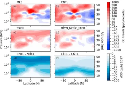
[image:6.612.94.519.88.378.2]

Figures 3a–3d show results from a simple ordinary least squares linear trend analysis on the MLS data and 3 model runs over the time period 2005–2017. The MLS observations show an increasing trend in the upper stratosphere due to stratospheric cooling and decreasing chlorine (e.g., Harris et al., 2015). In the middle and lower stratospheres the MLS observations show an increase in the SH and a decrease in the north, especially in the polar regions. This pattern of trends is well reproduced by the control run CNTL. The strong north-south asymmetry is similar to that derived in studies of stratospheric age-of-air over this period (e.g., Mahieu et al., 2014; Ploeger et al., 2015; Stiller et al., 2017). We are not attempting to derive robust trends over this short time period or attribute the causes of the trends, but we simply want to demonstrate that the model is able to reproduce the main features of the observed ozone variations. The results from run fDYN (Figure 3c) show the trend resulting from changes in chemistry, aerosols, and the solar cycle only over the period 2005–2017 (but with constant aerosol after 2014). The largest trends shown in Figure 3c, due to dynamics, have been removed, and there is an increasing trend almost everywhere. The trend in Figure 3d

(7)

is due only to changes in model chemistry, that is, prescribed mainly halogen-containing anthropogenic gases. This shows a clear increasing trend in ozone in the upper stratosphere due to declining chlorine. In the lower stratosphere, there is a large positive trend at SH midlatitudes, likely related to decreasing loss at the edge of the Antarctic ozone hole, though depletion at the pole is saturated and shows a near-zero trend.

4.2. Cause of Ozone Variations

Figure 4 shows the contributions of different model processes to changes in partial column ozone from 60°S–60°N from 1998 to 2017. The largest absolute variations occur in the lower stratospheric (and total) column where ozone is more abundant (see also Figures S5 and S6). Over all three levels the largest variations over this time period are caused by meteorology (temperature and winds). This includes large variations of up to ±5 DU in the lower stratosphere and the switch from the negative to positive anomaly in 2016/2017. The next largest impact over this time period is from the 11-year solar cycle in the upper and middle stratospheres.

[image:7.612.191.560.90.363.2]

For all altitude regions, and the total column, Figure 4 shows that the impact of the estimated trends in chlori-nated VSLS is small—less than 0.5 DU in the total column. Similarly, the impact of an assumed 0.5 ppt/decade increase in natural brominated VSLS has a small effect, though larger than for VSLS-Cl. Figures 3e and 3f illus-trate the effect of VSLS chlorine and bromine species, respectively. This is quantiﬁed from the difference in modeled ozone in 2017 between pairs of simulations with and without the respective VSLS trends. The addi-tional VSLS chlorine acts to deplete ozone in the upper stratosphere and high-latitude lower stratosphere. Bromine is only important in the lower stratosphere. The maximum impact is at high latitudes, but it has a larger impact at tropical latitudes than chlorine. The impact of VSLS halogens is larger under elevated SAD loading from volcanic eruptions. However, these panels show that with the current chemistry included in the model, halogenated VSLS do not have an especially large leverage to destroy ozone in the tropical lower stratosphere compared to other regions during this relatively short period, even considering the assumption

(8)

of constant aerosol after 2014 in the model simulations. This has to be borne in mind when looking for the ﬁngerprint of their impact on ozone loss.

5. Discussion and Conclusions

The results presented here update the work of Ball et al. (2018) in three important ways. First, in 2017 obser-vations of ozone in the extrapolar lower stratosphere show a large positive anomaly, especially in the SH. Inclusion of this additional year in the observational time series changes the interpretation of the ozone behavior from one of a downward trend to one of larger variability.

Second, we show that the observed variations in stratospheric ozone can be reproduced by a 3-D model and are therefore largely consistent with our understanding. While we cannot determine the cause of dynamical variations which are the main driver of the observed ozone changes, we can say that there appear to be no major shortcomings in the performance of the model.

Third, using a detailed stratospheric chemical model and realistic assumptions about the trend in chlorinated VSLS, we can exclude this as a possible cause of signiﬁcant lower stratosphere ozone depletion over the past decade or so based on known chemistry. Chlorine-catalyzed ozone depletion is relatively inefﬁcient in the extrapolar lower stratosphere in the absence of enhanced aerosol SAD and so is unlikely to cause large changes on this time scale. Even the assumption of a much larger chlorine VSLS trend would not produce an impact in our model.

Ball et al. (2018) suggested that positive trends in tropospheric ozone (together with positive trends in the upper stratosphere) may have compensated for the decline in lower stratosphere to result in near-zero observed total ozone trends (Weber et al., 2018). This was also discussed in Shepherd et al. (2014). As our study suggests a smaller trend in lower stratospheric ozone, this implies that positive tropospheric ozone trends are not required to explain the recent changes seen in the partial stratospheric columns as well as in total ozone.

Overall, the results presented here conﬁrm that ozone in the extrapolar lower stratosphere is largely under dynamical control, particularly over short time scales of a few years. The impact of chemical changes occurs on longer time scales. With our off-line CTM we are not able to diagnose the cause of dynamical variations and distinguish between variability and trends. CCM results have shown that ozone in the tropical lower stra-tosphere is sensitive to trends in tropical upwelling, which is predicted to lead to smaller column ozone values by the end of this century (Eyring et al., 2010). The results of Ball et al. (2018) and the work presented here show that there can be much variability associated with these expected long-term trends. Therefore, there is an important need for continued monitoring of ozone proﬁles throughout the lower stratosphere to detect and understand changes such as this.

References

Alsing, J., & Ball, W. (2017).“BASIC composite ozone time-series data”, Mendeley Data, v2. https://doi.org/10.17632/2mgx2xzzpk.2 Arfeuille, F., Luo, B. P., Heckendorn, P., Weisenstein, D., Sheng, J. X., Rozanov, E., et al. (2013). Modeling the stratospheric warming following

the Mt. Pinatubo eruption: Uncertainties in aerosol extinctions.Atmospheric Chemistry and Physics,13, 11,221–11,234. https://doi.org/ 10.5194/acp-13-11221-2013

Ball, W. T., Alsing, J., Mortlock, D. J., Rozanov, E. V., Tummon, F., & Haigh, J. D. (2017). Reconciling differences in stratospheric ozone composites.Atmospheric Chemistry and Physics,17(20), 12,269–12,302. https://doi.org/10.5194/acp-17-12269-2017

Ball, W. T., Alsing, J., Mortlock, D. J., Staehelin, J., Haigh, J. D., Peter, T., et al. (2018). Evidence for a continuous decline in lower stratospheric ozone offsetting ozone layer recovery.Atmospheric Chemistry and Physics,18(2), 1379–1394. https://doi.org/10.5194/acp-18-1379-2018 Chipperﬁeld, M. (2006). New version of the TOMCAT/SLIMCAT off-line chemical transport model: Intercomparison of stratospheric tracer

experiments.Quarterly Journal of the Royal Meteorological Society,132(617), 1179–1203. https://doi.org/10.1256/qj.05.51

Chipperﬁeld, M. P., Bekki, S., Dhomse, S., Harris, N. R. P., Hassler, B., Hossaini, R., et al. (2017). Detecting recovery of the stratospheric ozone layer.Nature,549(7671), 211–218. https://doi.org/10.1038/nature23681

Coddington, O., Lean, J., Pilewskie, P., Snow, M., & Lindholm, D. (2016). A solar irradiance climate data record.Bulletin of the American Meteorological Society,97(7), 1265–1282. https://doi.org/10.1175/BAMS-D-14-00265.1

Coldewey-Egbers, M., Loyola, D. G., Koukouli, M., Balis, D., Lambert, J.-C., Verhoelst, T., et al. (2015). The GOME-type total ozone essential climate variable (GTO-ECV) data record from the ESA climate change initiative.Atmospheric Measurement Techniques,8(9), 3923–3940. https://doi.org/10.5194/amt-8-3923-2015

Dee, D., Uppala, S., Simmons, A., Berrisford, P., Poli, P., Kobayashi, S., et al. (2011). The ERA-Interim reanalysis: Conﬁguration and performance of the data assimilation system.Quarterly Journal of the Royal Meteorological Society,137(656), 553–597. https://doi.org/10.1002/qj.828 Dhomse, S., Chipperﬁeld, M. P., Feng, W., Hossaini, R., Mann, G. W., & Santee, M. L. (2015). Revisiting the hemispheric asymmetry in

mid-latitude ozone changes following the Mount Pinatubo eruption: A 3-D model study.Geophysical Research Letters,42, 3038–3047. https://doi.org/10.1002/2015GL063052

Acknowledgments

(9)

Eyring, V., Cionni, I., Bodeker, G. E., Charlton-Perez, A. J., Kinnison, D. E., Scinocca, J. F., et al. (2010). Multi-model assessment of stratospheric ozone return dates and ozone recovery in CCMVal-2 models.Atmospheric Chemistry and Physics,10(19), 9451–9472. https://doi.org/ 10.5194/acp-10-9451-2010

Garane, K., Lerot, C., Coldewey-Egbers, M., Verhoelst, T., Koukouli, M. E., Zyrichidou, I., et al. (2018). Quality assessment of the ozone_cci climate research data package (release 2017)—Part 1: Ground-based validation of total ozone column data products.Atmospheric Measurement Techniques,11, 1385–1402. https://doi.org/10.5194/amt-11-1385-2018

Harris, N. R. P., Hassler, B., Tummon, F., Bodeker, G. E., Hubert, D., Petropavlovskikh, I., et al. (2015). Past changes in the vertical distribution of ozone—Part 3: Analysis and interpretation of trends.Atmospheric Chemistry and Physics,15(17), 9965–9982. https://doi.org/10.5194/ acp-15-9965-2015

Hossaini, R., Chipperﬁeld, M. P., Montzka, S. A., Leeson, A. A., Dhomse, S., & Pyle, J. A. (2017). The increasing threat to stratospheric ozone from dichloromethane.Nature Communications,8, 15962. https://doi.org/10.1038/ncomms15962

Hossaini, R., Chipperfield, M. P., Montzka, S. A., Rap, A., Dhomse, S., & Feng, W. (2015). Efficiency of short-lived halogens at influencing climate through depletion of stratospheric ozone.Nature Geoscience,8(3), 186–190. https://doi.org/10.1038/ngeo2363

Hossaini, R., Chipperﬁeld, M. P., Saiz-Lopez, A., Harrison, J. J., Glasow, R. v., Sommariva, R., et al. (2015). Growth in stratospheric chlorine from short-lived chemicals not controlled by the Montreal Protocol.Geophysical Research Letters,42, 4573–4580. https://doi.org/10.1002/ 2015GL063783

Mahieu, E., Chipperﬁeld, M. P., Notholt, J., Reddmann, T., Anderson, J., Bernath, P. F., et al. (2014). Recent northern hemisphere hydrogen chloride increase due to atmospheric circulation change.Nature,515(7525), 104–107. https://doi.org/10.1038/nature13857 Navarro, M. A., Atlas, E. L., Saiz-Lopez, A., Rodriguez-Lloveras, X., Kinnison, D. E., Lamarque, J. F., et al. (2015). Airborne measurements of

organic bromine compounds in the Paciﬁc tropical tropopause layer.Proceedings of the National Academy of Sciences of the United States of America,112(45), 13,789–13,793. https://doi.org/10.1073/pnas.1511463112

Oram, D. E., Ashfold, M. J., Laube, J. C., Gooch, L. J., Humphrey, S., Sturges, W. T., et al. (2017). A growing threat to the ozone layer from short-lived anthropogenic chlorocarbons.Atmospheric Chemistry and Physics,17(19), 11,929–11,941. https://doi.org/10.5194/acp-17-11929-2017

Ploeger, F., Riese, M., Haenel, F., Konopka, P., Müller, R., & Stiller, G. (2015). Variability of stratospheric mean age of air and of the local effects of residual circulation and eddy mixing.Journal of Geophysical Research: Atmospheres,120, 716–733. https://doi.org/10.1002/2014JD022468 Shepherd, T. G., Plummer, D. A., Scinocca, J. F., Hegglin, M. I., Fioletov, V. E., Reader, M. C., et al. (2014). Reconciliation of halogen-induced

ozone loss with the total ozone column record.Nature Geoscience,7(6), 443–449. https://doi.org/10.1038/ngeo2155

Solomon, S., Ivy, D. J., Kinnison, D., Mills, M. J., Neely, R. R., & Schmidt, A. (2016). Emergence of healing in the Antarctic ozone layer.Science,

353(6296), 269–274. https://doi.org/10.1126/science.aae0061

Stiller, G. P., Fierli, F., Ploeger, F., Cagnazzo, C., Funke, B., Haenel, F. J., et al. (2017). Shift of subtropical transport barriers explains observed hemispheric asymmetry of decadal trends of age of air.Atmospheric Chemistry and Physics,17(18), 11,177–11,192. https://doi.org/10.5194/ acp-17-11177-2017

Strahan, S. E., & Douglass, A. R. (2017). Decline in Antarctic ozone depletion and lower stratospheric chlorine determined from Aura Microwave Limb Sounder observations.Geophysical Research Letters,45, 382–390. https://doi.org/10.1002/2017GL074830 Weber, M., Coldewey-Egbers, M., Fioletov, V. E., Frith, S. M., Wild, J. D., Burrows, J. P., et al. (2018). Total ozone trends from 1979 to 2016

derived fromﬁve merged observational datasets—The emergence into ozone recovery.Atmospheric Chemistry and Physics,18(3), 2097–2117. https://doi.org/10.5194/acp-18-2097-2018

Weber, M., Dikty, S., Burrows, J. P., Garny, H., Dameris, M., Kubin, A., et al. (2011). The Brewer-Dobson circulation and total ozone from seasonal to decadal time scales.Atmospheric Chemistry and Physics,11(21), 11,221–11,235. https://doi.org/10.5194/acp-11-11221-2011 Werner, B., Stutz, J., Spolaor, M., Scalone, L., Raecke, R., Festa, J., et al. (2017). Probing the subtropical lowermost stratosphere and the tropical

upper troposphere and tropopause layer for inorganic bromine.Atmospheric Chemistry and Physics,17(2), 1161–1186. https://doi.org/ 10.5194/acp-17-1161-2017