8-23-2018
Low-Shot Learning for the Semantic Segmentation
of Remote Sensing Imagery
Ronald Kemker
Follow this and additional works at:https://scholarworks.rit.edu/theses
This Dissertation is brought to you for free and open access by RIT Scholar Works. It has been accepted for inclusion in Theses by an authorized administrator of RIT Scholar Works. For more information, please [email protected].
Recommended Citation
M.S. in Electrical Engineering, Michigan Technological University, 2011 A dissertation submitted in partial fulfillment of the
requirements for the degree of Doctor of Philosophy in the Chester F. Carlson Center for Imaging Science
College of Science
Rochester Institute of Technology August 23, 2018
Signature of the Author Accepted by
CERTIFICATE OF APPROVAL
Ph.D. DEGREE DISSERTATION
The Ph.D. Degree Dissertation of Ronald Kemker has been examined and approved by the dissertation committee as satisfactory for the
dissertation required for the Ph.D. degree in Imaging Science
Dr. Christopher Kanan, Dissertation Advisor Dr. Pengcheng Shi, External Chair
Dr. Carl Salvaggio Dr. Michael Gartley Date
Ronald Kemker Submitted to the
Chester F. Carlson Center for Imaging Science in partial fulfillment of the requirements
for the Doctor of Philosophy Degree at the Rochester Institute of Technology
Abstract
Deep-learning frameworks have made remarkable progress thanks to the creation of large annotated datasets such as ImageNet, which has over one million training images. Although this works well for color (RGB) imagery, labeled datasets for other sensor modalities (e.g., multispectral and hyperspectral) are minuscule in comparison. This is because annotated datasets are expensive and man-power intensive to complete; and since this would be impractical to accomplish for each type of sensor, current state-of-the-art approaches in computer vision are not ideal for remote sensing problems. The shortage of annotated remote sensing imagery beyond the visual spectrum has forced researchers to embrace unsupervised feature extracting frameworks. These features are learned on a per-image basis, so they tend to not generalize well across other datasets. In this disser-tation, we propose three new strategies for learning feature extracting frameworks with only a small quantity of annotated image data; including 1) self-taught feature learn-ing, 2) domain adaptation with synthetic imagery, and 3) semi-supervised classification. “Self-taught” feature learning frameworks are trained with large quantities of unlabeled imagery, and then these networks extract spatial-spectral features from annotated data for supervised classification. Synthetic remote sensing imagery can be used to boot-strap a deep convolutional neural network, and then we can fine-tune the network with real im-agery. Semi-supervised classifiers prevent overfitting by jointly optimizing the supervised classification task along side one or more unsupervised learning tasks (i.e., reconstruc-tion). Although obtaining large quantities of annotated image data would be ideal, our work shows that we can make due with less cost-prohibitive methods which are more practical to the end-user.
like to thank Kushal Kafle and Tyler Hayes for being a sounding board during my time here and for putting up with my antics in the lab. Fourth, I would like to thank the count-less number of people from previous assignments that have invested so much time into my development and made this opportunity possible. I would like to give a special shout-out to all of my military and civilian mentors, including Mike Roggemann, Chris Mid-dlebrook, Glen Archer, Nik Subotic, Tyler Erickson, Colin Brooks, Joel LeBlanc, John Valenzuela, Frank Scenna, Brian McKellar, Andrew Hoff, Ian Cameron, Wendy Kun-kle, Carl Brenner, Jeffrey Kwok, Paul Sebold, Michael Grogan, Michael Belko, Bobby Bankston, and the many others that have and continue to shape my personal and profes-sional career. Good luck to all of you, and your families, in your future endeavors.
Finally, Christine and I would both like to thank all of the friends that we have met here, especially the US/Canadian Air Force students and their families. You have provided a community that made our time here a bit easier and more enjoyable. Good luck to all of you and I hope that our paths cross again really soon!
Author Publications
†indicates that a modified version of this publication is included in this dissertation.
Refereed Publications
† Kemker, R., Luu, R., and Kanan C. (2018) Low-Shot Learning for the Semantic Segmentation of Remote Sensing Imagery. To appear in theIEEE Transactions on Geoscience and Remote Sensing (TGRS). 10.1109/TGRS.2018.2833808.
† Kemker, R., Salvaggio C., and Kanan C. (2018) Algorithms for Semantic Seg-mentation of Multispectral Remote Sensing Imagery using Deep Learning. ISPRS Journal of Photogrammetry and Remote Sensing - “Deep Learning for Remotely Sensed Data”. 10.1016/j.isprsjprs.2018.04.014.
• Kemker, R.and Kanan, C. (2018) FearNet: Brain-Inspired Model for Incremental Learning. In theProceedings for the Sixth International Conference for Learning Representations.
• Kemker, R., McClure, M., Abitino, A., Hayes, T., and Kanan, C. (2018) Measuring Catastrophic Forgetting in Neural Networks. In the Proceedings for the Thirty-Second Association for the Advancement of Artificial Intelligence (AAAI).
† Kemker, R.and Kanan C. (2017) Self-Taught Feature Learning for Hyperspectral Image Classification. IEEE Transactions on Geoscience and Remote Sensing (TGRS), 55(5): 2693-2705. 10.1109/TGRS.2017.2651639.
Workshop Papers
• Hayes, T.L., Kemker, R., Cahill, N.D., and Kanan C. (2018) New Metrics and Experimental Paradigms for Continual Learning. In Computer Vision and Pattern Recognition (CVPR) Workshop: Real World Challenges and New Benchmarks for Deep Learning in Robotic Vision.
Submitted/In-Review
Dedication iii
Dissertation Title & Abstract iv
Acknowledgements v
Author Publications vi
Table of Contents viii
List of Figures xii
List of Tables xvi
1 Introduction and Motivation 1
1.1 Context . . . 1
1.1.1 Self-Taught Learning . . . 1
1.1.2 Domain Adaptation . . . 2
1.1.3 Semi-supervised Learning . . . 3
1.2 Objectives . . . 3
1.3 Dissertation Layout . . . 4
1.3.1 Chapter 2: Self-Taught Feature Learning for Hyperspectral Image Classification (Objectives #1 and #2) . . . 4
1.3.2 Chapter 3: Algorithms for the Semantic Segmentation of Remote Sensing Imagery (Objective #2 and #3) . . . 5
1.3.3 Chapter 4: Low-Shot Learning for the Semantic Segmentation of Remote Sensing Imagery (Objective #4) . . . 5
2.2.1 Multi-scale ICA (MICA) . . . 14
2.2.2 Stacked Convolutional Autoencoders (SCAE) . . . 17
2.3 Experiments and Results . . . 19
2.3.1 HSI Datasets . . . 20
2.3.2 Experimental Setup . . . 22
2.3.3 Experimental Results . . . 25
2.3.4 Additional Experiments . . . 31
2.4 Discussion and Conclusions . . . 36
3 Algorithms for Semantic Segmentation of Multispectral Remote Sensing Im-agery using Deep Learning 39 3.1 Related Work . . . 42
3.1.1 Semantic Segmentation of RGB Imagery with Deep Networks . . 42
3.1.2 Deep-Learning for Non-RGB Sensors . . . 43
3.1.3 Semantic Segmentation of High Resolution Remote Sensing Im-agery . . . 44
3.1.4 MSI Semantic Segmentation Datasets for Remote Sensing . . . . 45
3.1.5 Deep Learning with Synthetic Imagery . . . 46
3.2 Methods . . . 47
3.2.1 Synthetic Image Generation using DIRSIG . . . 47
3.2.2 Fully-Convolutional Deep Networks for Semantic Segmentation . 49 3.2.3 Comparison Semantic Segmentation Algorithms . . . 53
3.3 RIT-18 Dataset . . . 56
3.3.1 Collection Site . . . 56
3.3.2 Collection Equipment . . . 57
3.3.3 Dataset Statistics and Organization . . . 58
3.4.1 Pre-Training the ResNet-50 DCNN on Synthetic MSI . . . 60
3.4.2 DCNN Fine-Tuning . . . 60
3.5 Experimental Results . . . 61
3.5.1 RIT-18 Results . . . 61
3.5.2 Band Analysis for RIT-18 . . . 65
3.6 Discussion . . . 65
3.7 Conclusion . . . 67
4 Low-Shot Learning for the Semantic Segmentation of Remote Sensing Im-agery 69 4.1 Related Work . . . 72
4.1.1 Self-Taught Feature Learning . . . 72
4.1.2 Semi-Supervised Learning . . . 73
4.2 Methods . . . 74
4.2.1 Multi-Loss Convolutional Autoencoder . . . 74
4.2.2 Semi-Supervised Multi-Layer Perceptron Neural Network . . . . 76
4.2.3 Adaptive Non-Linear Activations . . . 77
4.3 Experimental Setup . . . 78
4.3.1 Data Description . . . 78
4.3.2 Training Parameters . . . 80
4.4 Experimental Results and Discussion . . . 83
4.4.1 Single- vs. Multi-Loss CAE . . . 83
4.4.2 Stacked Feature Representations . . . 84
4.4.3 Multi-Sensor Fusion . . . 85
4.4.4 State-of-the-Art Comparison . . . 86
4.4.5 Dissimilarity Between Learned Features . . . 88
4.5 Conclusion . . . 91
5 Conclusion 92 A RIT-18: Dataset Creation Details 107 B RIT-18: Class Descriptions 110 B.1 Water/Beach Area . . . 110
B.2 Vegetation . . . 110
B.3 Roadway . . . 111
2.1 ICA filters learned from color (RGB) imagery. Most of the filters resem-ble Gabor filters. The green-red, dark-light, and yellow-blue opponency are an emergent phenomenon. . . 12 2.2 Our self-taught learning model using multiscale ICA (MICA) filters. This
framework learns low-level feature extractors from one (or more) hyper-spectral dataset(s) and then applies them to a separate target dataset. Mul-tiple datasets with varying GSDs can be used to make the filters scale invariant. . . 15 2.3 A visualization of the learned 15×15ICA filters from the Indian Pines
dataset. It was generated by summing across the spectral dimension of the filters (hundred of bands). Despite summing across all spectral di-mensions, this visualization still resembles the Gabor-like filters found in primary visual cortex. . . 17 2.4 This figure shows the CAE modules used in this chapter. The refinement
layer combines features from different parts of the network to provide a better reconstruction. . . 19 2.5 A two-layer stacked convolutional autoencoder. This figure shows how
a pre-trained network can extract features from labeled data and classify them. . . 20 2.6 The ground truth maps for Indian Pines 2.6(a), Salinas Valley 2.6(b), and
Pavia University 2.6(c) HSI datasets. . . 21 2.7 The classification maps for the Indian Pines dataset. Figures a-c were
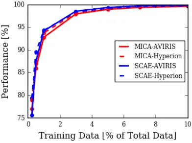
gen-erated with the SCAE-AVIRIS filters while Figures d-f were gengen-erated with the SCAE-Hyperion filters. These class maps correspond, respec-tively, to the following three training sets: 5% training data, 10% training data, and a training set commonly found in literature[1]. . . 27
the MICA-Hyperion filters. These class maps correspond to the following three training sets: 1% training data, 5% training data, and 50 samples per class respectively. . . 31 2.11 Results for the Salinas Valley dataset in terms of kappa statistic as a
func-tion of percent training samples per class. . . 32 2.12 The classification maps for the Pavia University dataset. Figures a-c were
generated with the SCAE-AVIRIS filters while Figures d-f were generated with the SCAE-Hyperion filters. These class maps correspond, respec-tively, to the following three training sets: 5% training data, 10% training data, and a training set commonly found in literature [2]. . . 34 2.13 Results for the Pavia University dataset in terms of kappa statistic as a
function of percent training samples per class. . . 35 2.14 This figure shows that the learned MICA filter bank is scale-invariant. The
solid lines represent the overall (red) and mean-class (blue) accuracies for the original data. The dashed lines represent the overall (red) and mean-class (blue) accuracies for the re-sized data. . . 36 2.15 This figure shows the classification performance of the Salinas Valley
dataset as the GSD is artificially changed through image resizing in terms of overall accuracy (OA), mean-class accuracy (AA), and kappa statistic (κ). The training set was fixed at 50 samples per class. . . 37 3.1 Our proposed model uses synthetic multispectral imagery to initialize a
3.4 Our Sharpmask model. The spatial dimensions of each module’s output are provided to illustrate that the refinement layer combines features from the feed-forward network (convolutional blocks) and the upsampled fea-tures in the reverse network to restore the original image dimensions. The output is a class probability matrix for each pixel. . . 50 3.5 Sharpmask refinement with batch normalization. This layer learns mask
refinement by merging features from the convolutionFiand segmentation
Mi networks. . . 51 3.6 Network Architecture incorporating RefineNet modules for semantic
seg-mentation. . . 52 3.7 RefineNet architecture. . . 53 3.8 Tetracam Micro-MCA6 mounted on-board the DJI-S1000 octocopter prior
to collection. . . 57 3.9 Class labels for RIT-18. . . 59 3.10 Class-label instances for the RIT-18 dataset. Note: The y-axis is
logarith-mic to account for the number disparity among labels. . . 59 3.11 Experimental results for Sharpmask and RefineNet models. These images
are small patches taken from the test orthomosaic. . . 64 4.1 Our proposed SuSA architecture for semantic segmentation of remote
sensing imagery. For feature extraction, SuSA uses our SMCAE model, a stacked multi-loss convolutional autoencoder that has been trained on un-labeled data using unsupervised learning. For classification, SuSA uses our semi-supervised multi-layer perceptron (SS-MLP) model. . . 70 4.2 MCAE model architecture. Dashed lines indicate where the mean-squared
error lossLj is calculated for layerj, and solid lines are the feed-forward
and lateral network connections where information is passed. The refine-ment layers (Fig. 2.4 are responsible for reconstructing the downsampled feature response. . . 74 4.3 Refinement layer used in CAE and MCAE. . . 76 4.4 The stacked multi-loss convolutional autoencoder (SMCAE) spatial-spectral
feature extractor used in this paper consists of two or more MCAE mod-ules. The red lines denote where features are being extracted, transferred to the next MCAE, and concatenated into a final feature response. . . 77 4.5 The semi-supervised multi-layer perceptron (SS-MLP) classification
4.10 Classification maps for SuSA on the Indian Pines and Pavia University datasets from the IEEE GRSS Data and Algorithm Standard Evaluation website. . . 90 A.1 Orthomosaic Processing Pipeline . . . 107 A.2 Difference between manufacturer’s affine transformation and our
perspec-tive transformation. The registration error in the affine transformation looks like a blue and red streak along the top and bottom of the parking lines, respectively. . . 108 C.1 The SCAE model used in this paper. Architecture details for each CAE
are shown in Fig. C.2. . . 113 C.2 The convolutional autoencoder (CAE) architecture used in SCAE. This
CAE is made up of several convolution and refinement blocks. The SCAE model in this paper uses three CAEs. . . 114 D.1 Heatmap visualization of the confusion matrices for all four models. Each
row is normalized to itself to highlight the most common errors. . . 116 D.2 Training (red) and validation (blue) loss and accuracy plots for
2.1 The convolutional autoencoder model used for this chapter wherez is ei-ther the number of spectral bands in the input image (first CAE) or the number of features extracted from the previous CAE (subsequent CAEs). The ‘Refinement 1’ layer is the feature response that will be passed to other CAEs and classified. Each convolutional layer consists of a convo-lution followed by batch normalization and ReLU activation. The refine-ment layer is outlined in Section 2.2.2. . . 23 2.2 The classification results for MICA and SCAE on the Indian Pines dataset.
The three training sets include #1) 5% per class, #2) 10% per class and #3) 50 samples per class (15 for smaller classes). We compare against state-of-the-art algorithms found in literature. Some statistics, including standard deviations, were not provided by the authors, so they could not be included. . . 26 2.3 The classification results for MICA and SCAE on the Salinas Valley dataset.
The three training sets include #1) 1% per class, #2) 5% per class and #3) 50 samples per class. We compare against state-of-the-art algorithms found in literature. Some statistics, including standard deviations, were not provided by the author, so they could not be included. . . 29 2.4 The classification results for MICA and SCAE on the Pavia University
dataset. The three training sets include #1) 5% per class, #2) 10% per class, and #3) a standard training set commonly found in literature. We compare against state-of-the-art algorithms found in literature. Some statistics, including standard deviations, were not provided by the author, so they could not be included. . . 33
2.7 RSA for SCAE-AVIRIS trained with an identical network initialization. The results are presented as the mean and standard deviation R2 on the test data from 10 cross-validation folds. This table shows R2 values for
predicting a column from a row. . . 36 3.1 Benchmark MSI semantic segmentation datasets, the year they were
re-leased, the sensor that collected it, its ground sample distance (GSD) in meters, and the number of labeled object classes (excluding the back-ground class). Our RIT-18 dataset is in bold. . . 46 3.2 Collection parameters for training, validation, and testing folds for RIT-18. 57 3.3 Data Collection Specifications . . . 58 3.4 Per-class accuracies as well as mean-class accuracy (AA) on the
RIT-18 test set. The two initializations used for our Sharpmask and RefineNet models include random initialization (Rdm) and a network initialized with synthetic data (Sim). We compare our results against the benchmark clas-sification frameworks listed in Section 3.5. . . 63 3.5 The effect of band-selection on mean-class accuracy (AA). For
compari-son, the last entry is the experiment from Table 3.4 which used all six-bands. 65 3.6 Performance of RefineNet-Sim on the RIT-18 test set using 4-band (VNIR)
and the full 6-band images. These results include per-class accuracies and mean-class accuracy (AA). . . 66 4.1 Various HSI sensors used in this paper to train and evaluate our SMCAE
4.5 Classification results on the Pavia University dataset using a single CAE and MCAE model trained on unlabeled AVIRIS data. These results were generated by training SS-MLP onLlabeled samples per class. Best per-formance for each experiment is in bold. . . 84 4.6 Classification performance using features extracted from SMCAE models
that were trained with data from different HSI sensors. . . 86 4.7 Results of low-shot learning experiment where the training set contains
onlyL=10 samples per class. . . 87 4.8 Performance comparison of SuSA against the other semi-supervised and
self-taught learning frameworks discussed in this paper. . . 88 4.9 Classification results for the Indian Pines and Pavia University datasets
from the IEEE GRSS Data and Algorithm Standard Evaluation website. . 89 4.10 Dissimilarity between the feature responses from all three SMCAE
object detection, semantic segmentation, etc. These breakthroughs have been made pos-sible by advancements in computer hardware (e.g. graphical processing units (GPUs), more efficient learning optimization schemes [3], fast and effective non-linear activations (e.g. rectified linear units (ReLU)), and massive labeled datasets such as ImageNet[4] and MSCOCO[5]. Although computer vision has made significant progress over the past several years, these frameworks still require large labeled datasets to learn discriminative features that generalize well.
1.1.1
Self-Taught Learning
The ImageNet Challenge uses an object recognition dataset that contains 1.2 million train-ing images distributed across 1,000 object classes. This dataset was considered by the computer vision community to be particularly challenging; and in 2012, the authors in [6] released the AlexNet DCNN which crushed the competition. This network-architecture opened the door to even deeper networks that have continued to push state-of-the-art de-velopment on the ImageNet challenge[7–9]. These DCNN frameworks have also been re-purposed to learn additional tasks with orders-of-magnitude less labeled data[10, 11].
Although deep-learning frameworks have been remarkably successful with color (RGB) imagery, supervised deep-learning frameworks for non-RGB sensors tend to not perform as well. This is because there is not an ImageNet-sized dataset for non-RGB image modal-ities such as multispectral (MSI) and hyperspectral imagery (HSI). Previous attempts to train DCNN frameworks to classify HSI resulted in mediocre performance because there are not enough samples to learn generalized features, so remote sensing researchers have embraced unsupervised spatial-spectral feature extractors such as stacked autoencoders. Although these frameworks have historically achieved state-of-the-art performance on in-dividual datasets, no work has demonstrated that these features transfer across multiple datasets/sensors. A real-time deployable framework should not learn a feature representa-tion on a per-image basis because of time and memory constraints, so it will need extract generalized features that are also discriminative enough to perform well across many im-ages.
In our work, we used self-taught learning to build spatial-spectral feature extractors for HSI classification. Instead of learning features that are specific to a single labeled dataset, self-taught learning uses large quantities of unlabeled data to learn discriminative features that generalize well. Once the framework is learned, it can be deployed to work across a variety of different datasets.
1.1.2
Domain Adaptation
The self-taught learning paradigm works well for some remote sensing scenes; however, very high resolution imagery requires the discriminative power of DCNN-based semantic segmentation frameworks. These models use combinations of convolution and spatial downsampling (pooling) layers that allow for the network to learn semantic information from large-scale scenes and to form associations between different objects present in the scene.
optimized to classify individual pixels and reconstruct the image data.
1.2
Objectives
This dissertation will address the training of supervised machine- and deep-learning frame-works with relatively small quantities of annotated remote sensing imagery (i.e. low-shot learning). The main objectives of our work include:
1. Develop universal feature extracting frameworks from large quantities of unlabeled data that work well across multiple datasets and sensors (i.e. self-taught learning).
(a) Evaluate the transferability of low- and high-level features built by self-taught learning frameworks (Chapters 2 and 4)
(b) Demonstrate that the discriminative power of these frameworks are more pow-erful when trained on large quantities of unlabeled data versus on the labeled data alone (Chapter 2 and 4)
(c) Demonstrate that these generalized features transfer across sensors (Chapter 2 and 4)
2. Establish new training/testing methodologies that enable the development of de-ployable classification frameworks for remote sensing imagery
(a) Identify issues with current training/testing methodologies in remote sens-ing literature which can affect the future deployability of these classification frameworks. (Chapter 2)
3. Develop universal feature extracting frameworks from large quantities of synthetic data (i.e. domain adaptation). (Chapter 3)
(a) Evaluate performance on new benchmark established in Chapter 3
(b) Demonstrate the utility of our learning strategy when model capacity increases 4. Develop modular self-taught feature learning paradigm for the semantic
segmenta-tion of remote sensing imagery. (Chapter 4)
(a) Improve original self-taught learning frameworks from Chapter 2 by incorpo-rating multiple reconstruction losses throughout the framework.
(b) Evaluate the discriminative power of these learned features learned and com-pare it to previous feature extraction methods presented in Chapter 2.
(c) Develop semi-supervised classification framework that works well with small quantities of annotated image data.
(d) Demonstrate that the improved feature extraction framework and a semi-supervised classifier yield state-of-the-art performance for the semantic segmentation of non-RGB remote sensing imagery.
1.3
Dissertation Layout
This dissertation consists of five chapters, including the introduction (Chapter 1) and con-clusion (Chapter 5).
1.3.1
Chapter 2: Self-Taught Feature Learning for Hyperspectral
Image Classification (Objectives #1 and #2)
1.3.2
Chapter 3: Algorithms for the Semantic Segmentation of
Re-mote Sensing Imagery (Objective #2 and #3)
Deep convolutional neural networks (DCNNs) have been used to achieve state-of-the-art performance on many computer vision tasks (e.g., object recognition, object detection, se-mantic segmentation) thanks to a large repository of annotated image data. Large labeled datasets for other sensor modalities, e.g., multispectral imagery (MSI), are not available due to the large cost and manpower required. In this chapter, we adapt state-of-the-art DCNN frameworks in computer vision for semantic segmentation for MSI imagery. To overcome label scarcity for MSI data, we substitute real MSI for generated synthetic MSI in order to initialize a DCNN framework. We evaluate our network initialization scheme on the new RIT-18 dataset that we present in this chapter. This dataset contains very-high resolution MSI collected by an unmanned aircraft system. The models initialized with synthetic imagery were less prone to over-fitting and provide a state-of-the-art baseline for future work.
1.3.3
Chapter 4: Low-Shot Learning for the Semantic Segmentation
of Remote Sensing Imagery (Objective #4)
gen-erate image annotations. Low-shot learning algorithms can make effective inferences despite smaller amounts of annotated data. In this paper, we study low-shot learning us-ing self-taught feature learnus-ing for semantic segmentation. We introduce 1) an improved self-taught feature learning framework for HSI and MSI data and 2) a semi-supervised classification algorithm. When these are combined, they achieve state-of-the-art perfor-mance on remote sensing datasets that have little annotated training data available. These low-shot learning frameworks will reduce the manual image annotation burden and im-prove semantic segmentation performance for remote sensing imagery.
1.4
Novel Contributions
Chapter 2: Self-Taught Feature Learning for Hyperspectral Image Classification
The main contribution of this chapter was to introduce the self-taught learning paradigm to the remote sensing community. We trained spatial-spectral feature extracting frame-works on large quantities of unlabeled hyperspectral imagery (HSI). The large quantities of data allow our frameworks to learn discriminative features that can transfer across datasets.
We used two feature extracting frameworks to demonstrate that our self-taught learn-ing paradigm is capable of transferrlearn-ing features across multiple datasets by achievlearn-ing state-of-the-art classification results on the Indian Pines, Salinas Valley, and Pavia Uni-versity datasets. One of these frameworks uses independent component analysis to build low-level feature extracting filters that resemble Gabor patterns (i.e. bar/edge detectors). The other is a stacked convolutional autoencoder framework that is capable of extracting deep spatial-spectral features from image data. We demonstrated that features from both frameworks can be transferred across different sensors through band-resampling.
We identified two problems with how HSI classification is currently performed in the remote sensing community. First, training and testing folds are traditionally built from the same HSI cube. This is ok with spectral-only classification; but if we want to include neighboring pixel information, there is a high chance of overlap between training and testing data. This can artificially inflate performance. Second, training/testing folds are built by randomly sampling available labeled data, and the results are reported as the mean/standard-deviation ofN runs.
Chapter 3: Algorithms for the Semantic Segmentation of Remote Sensing Im-agery
segmenta-available through the IEEE Geoscience and Remote Sensing Society (GRSS) evaluation server. This will standardize evaluation and push state-of-the-art development.
Chapter 4: Low-Shot Learning for the Semantic Segmentation of Remote Sens-ing Imagery
We introduced the semantic segmentation framework SuSA (self-taughtsemi-supervised
autoencoder). SuSA is designed to perform well on MSI and HSI data where image an-notations are scarce.
We developed the stacked multi-loss convolutional auto-encoder (SMCAE) model for spatial-spectral feature extraction in non-RGB remote sensing imagery. SMCAE uses unsupervised self-taught learning to acquire a deep bank of feature extractors. SMCAE is used by SuSA for feature extraction.
We propose the semi-supervised multi-layer perceptron (SS-MLP) model for the se-mantic segmentation of non-RGB remote sensing imagery. SuSA uses SS-MLP to clas-sify the feature representations from SMCAE, and SS-MLP’s semi-supervised mecha-nism enables it to perform well at low-shot learning.
We demonstrate that SuSA achieves state-of-the-art results on the Indian Pines and Pavia University datasets hosted on the IEEE GRSS Data and Algorithm Standard Evalu-ation website.
1.5
Related Publications
Portions of this dissertation have been published in the following outlets:
• Kemker, R., Salvaggio, C, and Kanan C. (2017) High-Resolution Multispectral Dataset for Semantic Segmentation.arXiv preprint arXiv:1703.06452.
• Kemker, R., Salvaggio C., and Kanan C. (2017) Algorithms for Semantic Seg-mentation of Multispectral Remote Sensing Imagery using Deep Learning. ISPRS Journal of Photogrammetry and Remote Sensing - “Deep Learning for Remotely Sensed Data”. 10.1016/j.isprsjprs.2018.04.014.
wavelets [14–16], extended morphological profiles [17], morphological attribute profiles [18], extended multi-attribute profiles (EMAP) [1], and rotation invariant spatial-spectral feature representations [19]. These features have major limitations and often require a great deal of tuning to get them to work well on a particular dataset. An alternative ap-proach is to train an algorithm that learns how to extract useful features directly from the pixels. Deep convolutional neural networks (CNNs) have been widely adopted in computer vision for this purpose, but they require large labeled datasets to train; other-wise, they will work poorly on test data. Existing labeled HSI datasets for remote sensing are minuscule in comparison to the color (RGB) datasets used in computer vision. This problem is compounded by the far greater dimensionality of pixels in HSI compared to RGB, making it difficult to use supervised feature learning techniques on today’s HSI datasets. However, unsupervised feature learning can be used because these techniques do not require labels. A variation of this approach is self-taught learning [20], which uses unsupervised learning to train a model by extracting features from large unlabeled datasets. The self-taught model is then applied to a target labeled dataset. The assumption behind self-taught models is that the features they learn to extract are generalizable, i.e., they will work well across datasets if their underlying natural statistics are similar. In
this chapter, we study two distinct self-taught learning algorithms for classifying pixels in HSI.
A number of researchers have used unsupervised learning to extract features from HSI data. The earliest of these did this by learning linear combinations of individual pixels using principal component analysis (PCA) [21] and independent component anal-ysis (ICA) [22–25]. These methods were pixel-specific, and did not include information about the neighborhood around the pixel. As the ground sample distance (GSD) for HSI improved, it was shown that spatial and spectral features could be combined to improve classification performance [26]. A number of algorithms have been used to extract spatial-spectral features from HSI data, including stacked autoencoders [2, 27–31], dictionary learning [32, 33], and ICA [34]. These methods discover salient information buried in the data.
The majority of published unsupervised feature learning frameworks involve learning spatial-spectral features from a single HSI dataset, breaking these feature responses up into test and train data, and then classifying that dataset [2, 15, 35–37]. In some cases, the features are learned on both training and testing data, which may skew results compared to what can be expected when the system is deployed [15, 36]. In self-taught learning for HSI classification, three steps are needed: 1) learn a set of filters from dataset #1, 2) use these filters to generate features from dataset #2, and then 3) classify dataset #2. Self-taught learning frameworks are more representative of an operational or deployed system since the test data is not used for unsupervised feature extraction or classifier training.
common algorithms for unsupervised feature learning in RGB images arek-means [38], sparse coding[39–41], and ICA [42, 43], with ICA generally yielding the best results in the literature.
Figure 2.1 shows filters learned using ICA on natural color images [44]. Each filter resembles Gabor filters that have been widely used to model simple cells in the human visual cortex. Red-green, blue-yellow, and light-dark opponency is an emergent phe-nomenon with ICA filters learned from RGB images, and this same kind of opponency is found in the human visual system [43]. The ICA algorithm used is a sparse coding algorithm that was designed to separate a signal into its statistically independent (non-Gaussian) components. ICA builds sparse features from whitened data by learning a set of orthonormal basis vectors.
ICA has been heavily used for HSI data analysis problems, including spectral unmix-ing [25, 45], target detection [46], clusterunmix-ing [34] (sometimes called unsupervised classi-fication), and classification [22, 23]. While spectral features learned from HSI data with ICA have been widely used, little work has been done to learn spatial-spectral features from neighborhood pixel information.
Figure 2.1: ICA filters learned from color (RGB) imagery. Most of the filters resemble Gabor filters. The green-red, dark-light, and yellow-blue opponency are an emergent phenomenon.
will also learn higher-level features not present in ICA. SAEs have become extremely prevalent in HSI classification literature [27, 28] including sparse [2], denoising [29], and convolutional [30, 31].
2.1.2
Self-Taught Learning
Traditional supervised classification methods use only labeled data, which is often scarce or difficult to obtain. To compensate, several alternative frameworks have been proposed that harness unlabeled data or data from other datasets. Semi-supervised methods use both labeled and unlabeled data from a dataset [54]. A commonly used semi-supervised approach in remote sensing is active learning. Active learning uses an initial prediction from a classifier to feed more training data back into the classifier [55–57]. Transfer-learning frameworks exploit labeled data from other datasets to improve the performance of the supervised classifier. The additional labeled data does not necessarily need to share class labels with the original dataset, but it should be sufficiently representative of the data that will be classified [58–60]. For RGB image analysis in computer vision, training CNNs on very large labeled datasets and then using them on smaller labeled datasets has been enormously successful.
EMAPs were used to automatically extract spatial-spectral features and classify the In-dian Pines and Pavia University datasets. In [15], the authors used combinations of three-dimensional Gabor wavelets to extract spatial-spectral features from the Indian Pines dataset. These fused filters reduced the number of redundant features, resulting in more discriminative features. Other papers have extended these successes by fusing large com-binations of different spatial-spectral features. One of the most successful papers iterated through 54 different sets of spectral (raw spectrum, PCA, linear discriminant analysis (LDA), and non-parametric weighted feature extraction) and spatial (morphological pro-files, Gabor, grey-level co-occurrence matrices (GLCMs), and segmented GLCMs) fea-tures [36]. This chapter still holds some of the best results for the Salinas Valley and Pavia University datasets; however, each of their state-of-the-art results were achieved with a different combination of spatial-spectral features. This highlights a need for methods that can extract features that generalize across datasets with minimal tuning.
Unsupervised feature learning frameworks require less tuning than hand-crafted fea-tures. These methods learn a set of spatial-spectral filters by analyzing natural scenes. Some of the most successful methods are sparse coding algorithms and stacked-sparse autoencoders (SSAEs). Spatially-weighted sparse coding uses neighboring pixel infor-mation to improve the performance of spectral unmixing in HSI data [33]. The author used the dominant end-member to classify a given pixel, achieving an impressive perfor-mance on the Indian Pines dataset. In [35], the author used SSAEs to extract deep features from the three labeled datasets featured in this chapter. Other frameworks have been de-veloped to automatically tune spatial-spectral filters that were previously hand-crafted to provide the optimal class separation [63]. While ICA has been extensively used for un-supervised spatial-spectral feature learning with RGB imagery, less work has been done with HSI data and most of it is concentrated solely on spectral features of a single pixel and ignore neighborhood information [22–25, 34].
spatial-spectral features from a single data source; however, these filters may not be representative of spatial-spectral features found in other datasets. In [2], the author transferred a set of filters learned from one HSI dataset onto another. Both of these datasets had the same GSD and were imaged by the same sensor, so the ability of the features to generalize to other sensors or GSDs is unclear.
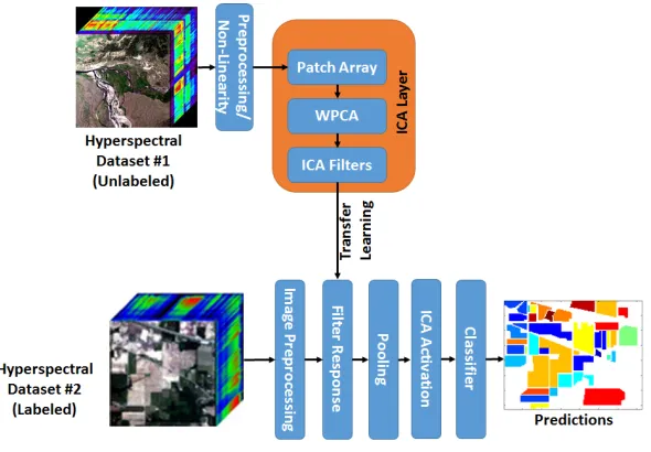
2.2
Self-Taught Learning Frameworks
We propose two distinct self-taught learning frameworks. MICA uses ICA to learn a shallow filter bank at multiple scales. SCAE is a deep neural network approach, which can potentially learn richer non-linear features than MICA. We use models with shal-low and deep feature representations to demonstrate the utility of our self-taught training methodology. Each model is trained on multiple unlabeled HSI datasets to add spatial-spectral variation to filters learned by the models. After training, both models are then used to extract features from the three labeled datasets, which are then fed to a classifica-tion algorithm. In this secclassifica-tion, we give high-level descripclassifica-tions for both models. Specific implementation details are provided in Section 2.3.
Acquiring large quantities of unlabeled HSI data is straight-forward thanks to gov-ernment and university sponsored websites containing open-source airborne/satellite im-agery. For this chapter, we used unlabeled data from the Airborne Visible / Infrared Imaging Spectrometer (AVIRIS) and Hyperion HSI sensors. The goal is to show that we can use self-taught learning to train a model that can extract features which generalize across datasets and sensors.
2.2.1
Multi-scale ICA (MICA)
Our proposed MICA model, illustrated in Figure 2.2, will learn a set of low-level feature extracting filters at multiple scales. When ICA is applied to image data, it tends to learn bar/edge, gradient, and corner detectors. MICA obtains robustness to multiple scales because it is trained on datasets collected at different altitudes. For example, a horizontal bar filter will detect the edge of a house or the outline of a long highway. These objects may be captured at different scales, but the same filter may respond similarly to them.
pro-Figure 2.2: Our self-taught learning model using multiscale ICA (MICA) filters. This framework learns low-level feature extractors from one (or more) hyperspectral dataset(s) and then applies them to a separate target dataset. Multiple datasets with varying GSDs can be used to make the filters scale invariant.
duces better behaved first-order natural image statistics [64]. This kind of transforma-tion is common when learning filters using ICA in RGB, LMS, and monochrome col-orspaces [42, 43, 61, 62, 65]. These functions resemble transformations done in the retina to help the human visual system handle large changes in luminance. Typically, a mono-tonically increasing function is used, with its shape resembling a logarithm. Here, we used the cumulative distribution function (CDF) of an exponential distribution for this pre-processing step, which others have also used with ICA [65]:
ri = 1−exp(−λi|xi|) (2.1)
wherexi is theispectral band of pixelx∈Rz, andλiis a parameter fit to the pixels from
band i using the unlabeled datasets. In preliminary experiments, we found this worked better than using two alternative functions that used logarithms [42, 61].
[image:34.612.181.476.122.327.2]anzp2 ×kN patch arrayR. Whitened PCA (WPCA) is then used to whiten the data and
reduce the dimensionality:
X=D−12ETR (2.2)
whereXis the whitened patch array,Eis the eigenvectors of the covariance matrixRRT, andDis a diagonal matrix containing the corresponding eigenvalues of theEmatrix [42]. Consistent with others [43,62,66], the first principal component (PC) is discarded because it mainly corresponds to the brightness across patches, and the corresponding eigenvalue is orders of magnitude larger than the other PCs, which hinders the ability of ICA to learn discriminative features. These steps result in X being a d ×kN patch array, where d
specifies the reduced dimension where d zp2. The value for d is found using cross-validation.
Next, ICA is used to learn ad×dlinear transformation matrixAfrom the whitened data, which makes the data linearly statistically independent. Our spatial-spectral filters are built by multiplying the ICA transformation matrixAwith the WPCA transformation, i.e., W=AD−12ET, whereWwill be ad×zm2 matrix, where the rows ofWcontain
the filters. Each row ofWis then reshaped to the correct spatial dimension, producing a collection of dfilters of size p×p×z [43]. A visualization of the filters learned using this procedure is shown in Figure 2.3. These low-level ICA feature extractors include Gabor-like bar/edge detectors, image gradients, and various spatial textures. Convolving am×n×zHSI with the learned filter bank, while using symmetric border padding, will yield am×n×darray of feature responses.
Subsequently, mean-pooling is applied to the feature response array to incorporate translation robustness into MICA. We convolve each channel of the ICA feature responses with ana×amean pooling filter. We used padding to preserve the spatial dimensions of the ICA filter response map.
Finally, we increased the discriminative utility of the MICA feature responses by ap-plying a non-linear function to them. Previous work has shown that the discriminative power of ICA filters for images can be increased by taking the absolute value of the filter responses and then applying a CDF-like function [43, 61, 67]. Following [61], we apply the CDF of an exponential distribution to the ICA filter responses
gi = 1−exp(−λi|qi|) (2.3)
where qi is the mean-pooled feature response of channel i and λi is the learned scale
parameter of the exponential distribution. Theλi parameters were fit using the unlabeled
Figure 2.3: A visualization of the learned15×15ICA filters from the Indian Pines dataset. It was generated by summing across the spectral dimension of the filters (hundred of bands). Despite summing across all spectral dimensions, this visualization still resembles the Gabor-like filters found in primary visual cortex.
2.2.2
Stacked Convolutional Autoencoders (SCAE)
As a form of deep neural network, SCAE can extract higher-level features than the ones extracted by MICA. SCAE is made up of several autoencoders, so it is important to un-derstand how they operate.
An autoencoder is a type of neural network that can be trained in an unsupervised manner to learn an encoded representation of the data. A typical autoencoderf is given byˆx=f(x),wherexis the input. It is trained to try to makeˆxas close toxas possible, i.e., to learn an identity function. Typically, an autoencoder will have internal constraints so that the hidden layers of its neural network will learn interesting features, e.g., sparsity constraints or a bottle neck. After training, the output of the hidden layers can be used as an alternative encoding of the data. While an autoencoder could be trained end-to-end as a deep network, which is often done when using bottle-neck constraints, each autoencoder in an SAE is typically trained individually. An autoencoder with a single hidden layer is given by
Recoveringˆxis then given by
ˆ
x=σ(W0h+b0) (2.5) whereW0is typically constrained such thatW0 =WT.
A CAE is an autoencoder variation in which the hidden layers are convolutional lay-ers [52]. This allows them to efficiently process image data. The output of a convolutional hidden layer is given by
H=σ(W∗X), (2.6) where∗denotes the convolution operation,Xis the input (e.g., a 3-tensor HSI image),W is a learned filter bank (a 4-tensor), andHis the output feature response map (a 3-tensor). For brevity, we have dropped the biases in the equations.
Autoencoders, including CAEs, can be stacked to learn a hierarchical features [30, 31, 52, 53]. When this is done with CAEs, it gives rise to the SCAE. The output of layerkin an SCAE is then given by
Hk=σ Wk∗Hk−1, (2.7) whereH0 =X. Each layer in an SCAE is trained individually to minimize reconstruction
error and then its encoding is used as the input to the next CAE layer.
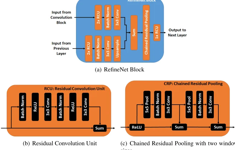
In this chapter, our SCAE uses three stacked CAE models; but as shown in Figure 2.4, the hidden layers we use are more complex than traditional CAEs. The feed-forward network resembles a traditional CNN architecture by incorporating max-pooling layers, which requires our model to upsample for reconstruction. In Figure 2.4, convolution #3 is a fully-connected layer followed by refinement modules [68], which are used to reconstruct the image. These modules use skip connections to merge low-level features from the feed-forward network with the high-level semantic features at the end of the network. This is followed by an upsampling operation until the image has been restored to its original dimensionality. As shown in Figure 2.4, each refinement module contains three separate convolution layers with trainable weights.
As shown in Figure 2.5, the feature responsesHk from each CAE are concatenated
and mean-pooled to introduce translation invariance. These features are then made unit length by dividing by the L2-norm. Since the dimensionality is much higher than the
Figure 2.4: This figure shows the CAE modules used in this chapter. The refinement layer combines features from different parts of the network to provide a better reconstruction.
2.3
Experiments and Results
We evaluated MICA and SCAE against three standard HSI benchmark datasets: Indian Pines, Salinas Valley, and Pavia University. The ground truth maps are shown in Figure 2.6. Section 2.3.1 discusses these datasets and the training sets that we will use to compare our frameworks against.
Section 2.3.2 lays out the specific network architectures proposed for this chapter and any other relevant information regarding training and evaluation. Section 2.3.3 lists the experimental results for both MICA and SCAE on the three benchmark datasets. Section 2.3.4 highlights some additional experiments that justify some of the decisions made for our proposed models.
Figure 2.5: A two-layer stacked convolutional autoencoder. This figure shows how a pre-trained network can extract features from labeled data and classify them.
2.3.1
HSI Datasets
We used unlabeled data from the AVIRIS and Hyperion HSI sensors to train our self-taught learning frameworks. We trained two MICA and SCAE models from each of the unlabeled data sources; MICA-AVIRIS, MICA-Hyperion, AVIRIS, and SCAE-Hyperion. We used three unlabeled datasets to train the MICA models and 20 datasets to train SCAE.
AVIRIS is an airborne sensor operated by NASA’s Jet Propulsion Laboratory. It has 224 visual/near-infrared (VNIR) and short-wave infrared (SWIR) spectral bands. The GSD varies with the elevation in which the data was collected.
Hyperion is a HSI sensor located on NASA’s EO-1 satellite. Hyperion data contains 242 VNIR/SWIR spectral bands; however, this experiment only used the 198 calibrated bands. The GSD of each HSI dataset is 30.5 meters, which is larger than all of the labeled datasets used in this chapter. The AVIRIS and Hyperion data is radiometrically calibrated using gain factors provided by NASA.
We denote the dimensionality of each labeled dataset by # of pixels × # of pixels
× # of bands. Bands that were in the atmospheric absorption region or bands with low signal-to-noise ratio (SNR) were removed.
Figure 2.6: The ground truth maps for Indian Pines 2.6(a), Salinas Valley 2.6(b), and Pavia University 2.6(c) HSI datasets.
104-108, 150-163, and 220-224 were removed due to atmospheric absorption or low SNR. The ground-truth contains 16 classes of different crops and crop-mixtures. Indian Pines has a GSD of 20 meters. Our self-taught learning algorithms were compared against three common training sets including #1) 5% per class[15], #2) 10% per class[33], and #3) a common training set containing 50 samples per class (except with a few smaller classes where 15 samples are reserved for training[1]).
Salinas Valley, Figure 2.6(b), is a512×217×204dataset that contains 16 ground-truth classes related to crops at different stages in their growth. The original dataset has 224-bands, but bands 108-112, 154-167, and 224 were removed due to atmospheric absorption or low SNR. The GSD for Salinas Valley is 3.7 meters. Our algorithms were compared against three standard training sets including #1) 1% per class[35], #2) 5% per class[36], and #3) 50 samples per class [36].
Pavia University, Figure 2.6(c), is a610×610×103dataset that was collected during a campaign flown over Northern Italy. The original dataset was band-resampled from 115 bands to 103 bands. Pavia University has 9 ground truth classes containing a mixture of man-made and natural scenery. The GSD for Pavia University is 1.3 meters. Our algo-rithms were compared against three common training sets including #1) 5% per class[36], #2) 10% per class[16], and #3) a custom training set commonly used in literature [2].
Spectrometer (ROSIS) sensor which only operates in the VNIR spectral range.
2.3.2
Experimental Setup
MICA Setup and Parameters
The MICA ICA filter size is fixed tom = 15across every dataset, which worked well in preliminary experiments. MICA’s mean pooling layer uses a11×11filters. We trained MICA using unlabeled datasets that came from different sensors. MICA-AVIRIS is solely trained with data from the AVIRIS sensor and MICA-Hyperion solely from data from the Hyperion sensor. In both cases, the filters were created by extracting 5,000 random patches from each of the three unlabeled datasets (15,000 patches total). The unlabeled AVIRIS datasets are orthorectified, so these rotated images have gaps in the corners with no data, and we did not extract patches from these empty regions. This quantity of data was sufficient to learn low-level bar/edge filters since these features can be found in most scenes.
SCAE Setup and Parameters
We trained two separate SCAE networks from AVIRIS (SCAE-AVIRIS) and Hyperion (SCAE-Hyperion) data. Each SCAE network stacks three CAEs with an identical archi-tecture. This architecture is outlined in Table 2.1. The last hidden layer of the preceding CAE becomes the input of the following CAE.
Each convolution module in Table 2.1 uses convolution followed by batch normaliza-tion and ReLU activanormaliza-tion. Batch normalizanormaliza-tion is a regularizanormaliza-tion technique that speeds up and stabilizes training by reducing internal covariate shift [73]. Every convolutional layer is randomly initialized with a zero-mean normal distribution [74].
The only pre-processing step for the unlabeled data is subtracting the channel mean and dividing by the channel standard deviation. This mean and standard deviation is stored and applied to the labeled data. SCAE was trained by extracting 2,000 16×16
Convolution 2 m2 × n
2 ×512 3×3×512
Max Pooling 2 m4 × n
4 ×512 2×2
Convolution 3 m4 × n
4 ×512 3×3×512
Max Pooling 3 m8 × n
8 ×512 2×2
Convolution 4 m8 × n
8 ×1024 1×1×1024
Refinement 3 m4 × n
4 ×512 3×3×512
Refinement 2 m2 × n
2 ×512 3×3×512
Refinement 1 m×n×256 3×3×256
Output m×n×z N/A
Each CAE was trained independently using the Adam optimizer with Nesterov momen-tum [3] and a mean-squared-error cost function. We used an initial learning rate of 2e-3 and dropped the learning rate by a factor of 10 (four times) as the validation loss plateaued. After learning its filters, each labeled dataset is passed through the SCAE network. These feature responses are concatenated, fed through a 5×5mean-pooling layer, and normalized with theL2-norm. WPCA is used to reduce the dimensionality of the feature
Band-Resampling
Band-resampling is used to maximize large quantities of unlabeled, open-source data. For MICA, filters are learned from the unlabeled data and then resampled to match the spectral bands of the target (labeled) data. For SCAE, the network is trained on the unlabeled data and the labeled data is resampled so it can be passed through the network. When deployed, unlabeled data from the sensor would be used to build these feature extracting frameworks.
Band-resampling could also be useful to take advantage of existing training data. For example, if we increased the spectral resolution of our sensor, we may be able to upsample existing labeled datasets in order to increase the quantity of annotated data. Labeled data is expensive and difficult to come by.
Classification
The training/testing sets were built by randomly sampling the feature responses generated by our MICA and SCAE frameworks. The number of samples extracted for training data was selected based on current state-of-the-art solutions found in literature, and a plot for each labeled dataset was generated to illustrate mean per-class accuracy as a function of percent of training samples. These feature responses were classified using a radial basis function SVM (RBF-SVM). Cross-validation was used to determine the optimal penalty term C and kernel width (γ) hyperparameters. For MICA, the feature responses were flipped across the horizontal axis to augment the training data.
The peak performance for the MICA framework in Section 2.3.3 was achieved by us-ing a different number of learned filters, which corresponds to the number of PCs retained during Section 2.2.1. If there are too many PCs, then the learned ICA filters will be noisy and less discriminative. We found that the ideal number differed for each labeled dataset, since they all cover different spectral bands and have a different quantity of labeled data available. For a deployable system, where the size of the image and spectral bands are fixed, the number of filters can be easily determined through cross-validation and fixed for future classification. In this chapter, we cross-validated by a step-size of 5 filters to determine the optimal quantity; however, adding or removing a few filters will not have a major impact on classification performance.
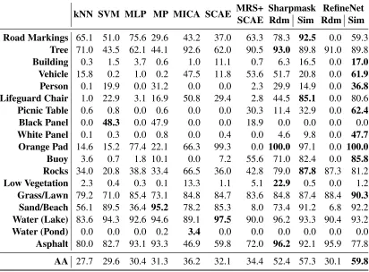
selected because it takes both overall and mean-class accuracy into account. Finally, we provide classification maps for the three state-of-the-art comparisons for each dataset.
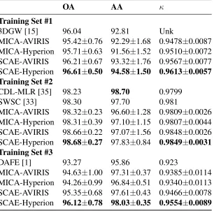
Indian Pines
Table 2.2 compares MICA and SCAE to state-of-the-art solutions for the Indian Pines dataset found in literature. We used the first 210 feature extracting filters for the MICA framework. The first training set, 5% training data, is compared against a spatial/spectral feature extraction method that uses three-dimensional Gabor wavelets (3DGW) [15]. The second training set, 10% training data, is compared against a spatially weighted sparse coding (SWSC) unmixing approach [33]. The third training set, 50 samples per class (except 3 smaller classes that use 15 samples per class), is compared to a paper that uses extended morphological attribute profiles for supervised feature extraction (DAFE) [1]. Contextual deep learning multinomial logistic regression (CDL-MLR) had a percent higher mean class accuracy for the second training set. Our classifier was cross-validated by using overall accuracy as the metric, and our algorithm yielded state-of-the art results for this metric. Overall, our self-taught learning frameworks, especially SCAE, proved to be more discriminative than the algorithms listed above.
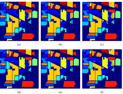
Figure 2.7 shows classification maps for the three training sets in Table 2.2 using our SCAE models. The majority of the errors reside in the pixel edges between classes, espe-cially between contiguous classes. Possible causes include adjacency effect and feature blurring with the mean-pooling layer. The errors between frameworks are not consistent, suggesting that ensembling may improve classification performance.
per class (15 for smaller classes). We compare against state-of-the-art algorithms found in literature. Some statistics, including standard deviations, were not provided by the authors, so they could not be included.
OA AA κ
Training Set #1
3DGW [15] 96.04 92.81 Unk
MICA-AVIRIS 95.42±0.76 92.29±1.68 0.9478±0.0087 MICA-Hyperion 95.71±0.63 91.56±1.52 0.9510±0.0072 SCAE-AVIRIS 96.21±0.67 93.32±1.76 0.9567±0.0077 SCAE-Hyperion 96.61±0.50 94.58±1.50 0.9613±0.0057 Training Set #2
CDL-MLR [35] 98.23 98.70 0.9799 SWSC [33] 98.30 97.70 0.981
MICA-AVIRIS 98.32±0.23 96.60±1.28 0.9809±0.0026 MICA-Hyperion 98.31±0.39 97.10±1.15 0.9807±0.0044 SCAE-AVIRIS 98.66±0.22 97.07±1.56 0.9848±0.0026 SCAE-Hyperion 98.68±0.27 97.83±0.84 0.9849±0.0031 Training Set #3
DAFE [1] 93.27 95.86 0.923
MICA-AVIRIS 94.63±1.00 97.31±0.37 0.9385±0.0114 MICA-Hyperion 94.26±0.99 96.84±0.51 0.9340±0.0113 SCAE-AVIRIS 95.35±0.68 97.61±0.43 0.9466±0.0078 SCAE-Hyperion 96.12±0.78 98.03±0.35 0.9554±0.0089
on larger GSD imagery, which is why there is a slight improvement on smaller training sets.
[image:45.612.172.478.204.506.2](d) (e) (f)
Figure 2.7: The classification maps for the Indian Pines dataset. Figures a-c were gen-erated with the AVIRIS filters while Figures d-f were gengen-erated with the SCAE-Hyperion filters. These class maps correspond, respectively, to the following three train-ing sets: 5% traintrain-ing data, 10% traintrain-ing data, and a traintrain-ing set commonly found in literature[1].
Salinas Valley
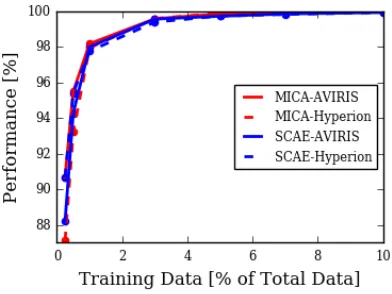
Figure 2.8: Results for the Indian Pines dataset in terms of kappa statistic as a function of percent training samples per class.
the HSI data with features from morphological profiles and segmented GLCM features. The third training set combines the features from the second training set along with Gabor and non-segmented GLCM features. MICA and SCAE both exceeded all earlier methods. Figures 2.9 and 2.10 show the classification maps for the three training sets in Table 2.3 using both our SCAE and MICA models respectively. The results indicate that our self-taught learning frameworks perform well on the fine-grain material identification task (lettuce at different growth stages and fallow conditions). The small error that is present mostly resides in the untrained grapes and untrained vineyards classes, which may have similar spectral characteristics.
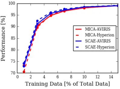
The kappa statistic for the Salinas Valley dataset is shown in Figure 2.11. Both of our frameworks work well for the Salinas Valley dataset, even with a low number of training samples. The close performance between MICA and SCAE indicates that low-level spatial-spectral features from MICA may be sufficient for this particular dataset.
SCAE-Hyperion 97.98±0.36 98.41±0.30 0.9776±0.0040
Training Set #2
GLCM+ [36] 98.61 Unk Unk
MICA-AVIRIS 99.87±0.03 99.82±0.12 0.9985±0.0008 MICA-Hyperion 99.90±0.05 99.88±0.06 0.9989±0.0005
SCAE-AVIRIS 99.75±0.06 99.69±0.09 0.9972±0.0007 SCAE-Hyperion 99.75±0.07 99.71±0.08 0.9973±0.0008
Training Set #3
GLCM+ [36] 95.41 Unk Unk
MICA-AVIRIS 97.15±0.56 98.57±0.29 0.9683±0.0062 MICA-Hyperion 95.95±0.66 98.34±0.24 0.9549±0.0073 SCAE-AVIRIS 98.06±0.45 98.94±0.22 0.9784±0.0050
SCAE-Hyperion 97.50±0.54 98.85±0.22 0.9722±0.0060
Pavia University
(a) (b) (c) (d) (e) (f)
Figure 2.9: The classification maps for the Salinas Valley dataset. Figures a-c were gen-erated with the AVIRIS filters while Figures d-f were gengen-erated with the SCAE-Hyperion filters. These class maps correspond, respectively, to the following three train-ing sets: 1% traintrain-ing data, 5% traintrain-ing data, and 50 samples per class.
Figure 2.12 shows the classification maps for the three training sets in Table 2.4 using SCAE features. There are only minor errors, which include confusing shadows for trees and bare soil for meadows.
Figure 2.10: The classification maps for the Salinas dataset. Figures a-c were generated with the MICA-AVIRIS filters while Figures d-f were generated with the MICA-Hyperion filters. These class maps correspond to the following three training sets: 1% training data, 5% training data, and 50 samples per class respectively.
2.3.4
Additional Experiments
Scale-Invariance of MICA
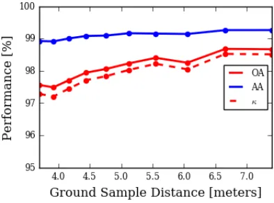
Earlier, we stated that the MICA filter-band is somewhat scale-invariant. Despite all three labeled datasets having different GSDs, MICA performed well on them. This is because some of the filters learned by MICA-AVIRIS and MICA-Hyperion resemble Gabor-type edge detectors at various sizes. One of these filters can work well at detecting a building from an image taken by an airborne sensor and could work just as well at detecting a long road imaged by a satellite sensor. MICA-AVIRIS is even more scale-invariant because it learns filters from a variety of datasets taken at different GSDs.
To prove our hypothesis, we re-sized the Indian Pines data and ground-truth map by half the original size. As a fair comparison, we used the same MICA-AVIRIS filters discussed in Section 2.3.3. In Figure 2.14, we see that re-sizing the image had a minimal impact on the classification performance, which could indicate that the filters work just as well across different scales. The minor differences in performance are likely due to re-size interpolation errors.
clas-Figure 2.11: Results for the Salinas Valley dataset in terms of kappa statistic as a function of percent training samples per class.
sification performance when the GSD of the Salinas Valley dataset is artificially changed through image re-sizing. During this experiment, the training size was fixed at 50 samples per class. There was a minor increase in performance due to image blurring; however, the overall performance of the MICA filter bank indicates that there is some resistance to scale-invariance.
Representation Similarity Analysis
How similar are the features learned across sensors and models? To address this question, we performed a representation similarity analysis (RSA) [75, 76] to compare the features extracted by the MICA and SCAE frameworks across sensors. RSA is a quantitative measure used by neuroscientists to assess the similarity of features from multiple models (or sources). Since MICA and SCAE have different dimensionality, we used reduced-rank regression (RRR) [77, 78] to do our RSA analysis. RRR is ordinary least-squares (OLS) regression with a low-rank constraint. This approach allows us to build a linear regression model from feature representation X to feature representation Y. We can then assess goodness of fit on test data to determine how well Y’s features can be reconstructed from X’s. If this can be done well, then X is considered to contain the same feature information as Y. Note that Y may only contain a subset of the features in X, so this regression analysis must be done from Y to X as well.
[image:51.612.225.421.130.277.2]SCAE-Hyperion 99.41±0.15 99.01±0.31 0.9921±0.0021
Training Set #2
3DSW [16] 99.30±0.12 98.63±0.23 0.9907±0.0016 MICA-AVIRIS 99.70±0.07 99.39±0.17 0.9961±0.0009 MICA-Hyperion 99.78±0.08 99.51±0.18 0.9971±0.0010 SCAE-AVIRIS 99.88±0.05 99.77±0.12 0.9984±0.0006
SCAE-Hyperion 99.81±0.06 99.65±0.13 0.9975±0.0008
Training Set #3
[image:52.612.172.477.204.491.2]SSAE [2] 98.63±0.17 97.64±0.22 0.9822±0.0013 MICA-AVIRIS 99.69±0.11 99.72±0.09 0.9957±0.0014 MICA-Hyperion 99.72±0.12 99.79±0.11 0.9962±0.0016 SCAE-AVIRIS 99.85±0.06 99.89±0.06 0.9980±0.0008 SCAE-Hyperion 99.88±0.05 99.87±0.06 0.9984±0.0006
Table 2.5: A comparison of the filter transfer learning experiment done in [2] and our MICA and SCAE models. The training set included 50 samples per class.
OA AA κ
SSAE [2] 91.96±0.87 93.52±0.42 0.9025±0.0112 MICA-AVIRIS 92.87±1.11 94.79±0.64 0.9067±0.0142 MICA-Hyperion 93.92±1.38 95.58±0.64 0.9203±0.0177 SCAE-AVIRIS 94.30±1.13 96.82±0.54 0.9253±0.0145 SCAE-Hyperion 95.84±0.94 96.56±0.51 0.9451±0.0123
from X’s. First the regularized OLS regression is computed, i.e.,
BOLS = X>X+λI −1
(a) (b) (c) (d) (e) (f)
Figure 2.12: The classification maps for the Pavia University dataset. Figures a-c were generated with the SCAE-AVIRIS filters while Figures d-f were generated with the SCAE-Hyperion filters. These class maps correspond, respectively, to the following three training sets: 5% training data, 10% training data, and a training set commonly found in literature [2].
whereX is the data we are fitting,Y is the data we are making the prediction on, andλ
is the L2-regularization penalty term. Then, PCA is performed on YˆOLS = BOLSX to
obtain the firstrPCsUr. The RRR solution is given by
BRRR=BOLSUrU>r, (2.9)
whereBRRRis used as a one-way linear mapping between feature representations.
Table 2.6 shows the coefficients of determination (R2) for the input X and the pre-dicted outputYˆRRR =BRRRX. We performed a 10-fold cross-validation using the MICA
and SCAE feature responses from the Pavia University dataset and reported theR2values
for the test data in terms of mean and standard deviation across all folds. The vertical and horizontal axes are the feature responses we fit and predicted respectively. We cross-validated for the optimal rankrand L2 regularization penalty termλ.
Table 2.6 shows that the low-level MICA features learned from both AVIRIS and Hyperion sensors are very similar to each other. Also, the MICA features can be predicted from the SCAE fairly accurately (R2 >0.9in all cases). However, MICA does a relatively
poor job predicting the output of SCAE. This suggests that SCAE produces many of the feature responses of MICA, but MICA omits some of the higher-level features that SCAE generates.
Figure 2.13: Results for the Pavia University dataset in terms of kappa statistic as a func-tion of percent training samples per class.
Table 2.6: RSA between MICA and SCAE feature responses built from Pavia University (see Section 2.3.4). This table showsR2 values for predicting a column (Y) from a row (X). A value of 1 means a perfect fit. The results are presented as the mean and standard deviation R2 on the test data from 10 cross-validation folds. Because test data is being
studied, the diagonal is not necessarily all 1s.
MICA Framework SCAE Framework
#1 AVIRIS #2 Hyperion #3 AVIRIS #4 Hyperion
#1 1.000±0.000 0.982±0.000 0.411±0.004 0.388±0.006
#2 0.974±0.001 1.000±0.000 0.431±0.004 0.421±0.006
#3 0.921±0.002 0.935±0.002 0.999±0.000 0.740±0.002
#4 0.915±0.002 0.927±0.002 0.730±0.001 0.999±0.000
Figure 2.14: This figure shows that the learned MICA filter bank is scale-invariant. The solid lines represent the overall (red) and mean-class (blue) accuracies for the original data. The dashed lines represent the overall (red) and mean-class (blue) accuracies for the re-sized data.
Table 2.7: RSA for SCAE-AVIRIS trained with an identical network initialization. The results are presented as the mean and standard deviation R2 on the test data from 10 cross-validation folds. This table showsR2values for predicting a column from a row.
Set #1 Set #2 Combined
Set #1 0.9987±0.0000 0.8269±0.0010 0.7966±0.0014
Set #2 0.8157±0.0010 0.9987±0.0000 0.8074±0.0015
Combined 0.8090±0.0011 0.8290±0.0012 0.9987±0.0000
features, but there was only a small decrease in similarity.
2.4
Discussion and Conclusions
state-of-Figure 2.15: This figure shows the classification performance of the Salinas Valley dataset as the GSD is artificially changed through image resizing in terms of overall accu-racy (OA), mean-class accuaccu-racy (AA), and kappa statistic (κ). The training set was fixed at 50 samples per class.
the-art results across all of the datasets. MICA and SCAE can learn filters from datasets with different GSDs making them robust to changes in scale.
The low-level features learned by MICA yielded superior results compared to the deeper stacked autoencoder architectures found in [2, 27–30]. This further demonstrates, as is true in any machine or deep learning problem, that the diversity and quantity of the training data can be just as important as the depth of our network. In most cases, our SCAE model yielded superior performance to our MICA model, showing that higher-level features can be advantageous in some cases.
[image:56.612.225.422.131.277.2]such as parts, objects, and the semantic relationship between pixels and spectral channels. High-level feature extractors will likely have more discriminative power than shallow ones, but they take longer to train and are often slower to run.
As we have demonstrated, self-taught learning can be useful for HSI classification. It al
![Table 2.5: A comparison of the filter transfer learning experiment done in [2] and ourMICA and SCAE models](https://thumb-us.123doks.com/thumbv2/123dok_us/64799.6139/52.612.172.477.204.491/table-comparison-lter-transfer-learning-experiment-ourmica-models.webp)