D a ta A n a ly sis In fr a str u c tu r e
for
G r a v ita tio n a l W ave A str o n o m y
By
Antony Charles Searle
December 2, 2004
D e c la ra tio n
I certify that the work contained in this thesis is my own original research,
produced in collaboration with my supervisor—Dr Susan M. Scott. All ma
terial taken from other references is explicitly acknowledged as such. I also
certify that the work contained in this thesis has not been submitted for any
other degree.
Antony Charles Searle
A c k n o w le d g e m e n ts
It was the best of times, it was the worst of times, it was the age of wisdom, it was the age of foolishness, it was the epoch of belief, it was the epoch of incredulity, it was the season of light, it was the season of darkness, it was the spring of hope, it was the winter of despair, we had everything before us, we had nothing before us, we were all going direct to Heaven, we were all going direct the other way— in short, the period was so fa r like the present period. that some of its noisiest authorities insisted on its being received, for good or fo r evil, in the superlative degree of comparison only.
— Charles Dickens, A Tale of Two Cities. These last few years have been the worst of my life: watching my mother Christine slowly consumed by cancer, my brush with history in Washington on a sunny Tuesday in September, and the very personal war on terror that followed. So special thanks is due to the people who also made these years the best of tim es: 1
Susan Scott (‘for Gochs sake, don’t say thatV), my indefatigable one- woman supervisor, funding body, travel agent, motivator, defender, coach and friend.
David McClelland, for his supervision, and for keeping the whole an tipodean gravitational-wave show on the road.
Those who shared my offices and kept the air crackling with ‘eclectricity’: Mike Ashley (and the Bone of Contention, and Other Tales), Benedict Cusack ('do you think it’s an ostrich farm ?’), Ingrid Irmer (into every generation a Com puter Slayer is born), and Andrew Moylan ('I can’t work out what this thing on my forehead is’). They left ‘Surly’ Searle less so than they found him.
IV
Those at my LIGO homes-away-from-home: at Caltech, Albert Lazzarini (‘American-Indian and Indian-American don't commute. They’re, like, ih.'), Kent Blackburn (‘I might engage in a little biological warfare of my own’), Ed Maros (who insisted the fault lay with Tel), Phil Ehrens (who insisted the fault lay with C + + ), Isaac Salzman (who found the fault), the faultless Peter Shawhan, and the whole LDAS team; at PennState, Sam Finn (‘when I get home at night I need a dog to kick, and [name withheld] can be that dog’) and Patrick Sutton (who drove all day to collect me after September 11. then nearly hit an eighteen-wheeler on the way back); at UT-Brownsville, Joe Romano (simply the nicest g u y ... ’nuff said), Warren Anderson (‘you can’t be that gullible’), and John Whelan (who has said so many things so quickly th at I only remember the gist of them).
Philip Charlton, Australia's ‘mole’ in LIGO data analysis, fits most of the above categories, and is a one-man cultural beachhead.
Anna Weatherly (‘can you say th a t again, slowly?’) for her counsel, Dr Alison McIntyre for an efficacious pharmacopoeia, and Coca-Cola Amatil for putting life’s necessities in a contour bottle.
My friends at the Canberra Speculative Fiction Guild, in particular the asvnchronous Maxine MacArthur, Michael Barry (wink-wink, nod-nod. say- no-more), the punctual Alan Price, and the lycanthromorphilic (?) Robbie Matthews. I’m not sure if they reciprocate: ‘The CSFG would like to ac knowledge the efforts of the following people:... Alan [sic] Searle... for addi tional proofing.’— Elsewhere (ed. Michael Barry), CSFG Publishing.
I don't know Fred Raab very well, but this overheard meta-quote is too good to pass up: ‘So my quote in her thesis is going to be th at LIGO looks like a sewage plant.'
A b s tr a c t
Interferometric gravitational wave observatories are coming on-line around the world, sensitive to infinitesimal ripples propagating through space-time itself. D ata analysis assumes an unusual importance in gravitational wave astronomy; all predicted gravitational wave signals from plausible astrophys- ical scenarios will be at the margins of detectability for current instruments, and even as sensitivities improve, the m ajority of signals will remain in this regime.
The immediate goal of current observatories is to make the first widely- accepted direct detection of gravitational waves; to this end, I have made sig nificant contributions to the d ata analysis systems of leading observatories, spanning design, implementation, testing, and characterisation of compo nents ranging from basic signal-processing to tailored d ata conditioning op erations. These components have been employed to produce several worlds- best direct observational upper limits on gravitational wave phenomena.
C o n te n ts
1 Introduction 1
1.1 Review...
2
1.2 Publications...
4
1.3 Overview...
6
1
D a t a C o n d i t i o n i n g
7
2 The LDAS data conditioning API 92.1 The LIGO Data Analysis System (LDAS) ... 10
2.1.1
A P I s ... 11
2.1.2
Command language... 11
2.2 Design and evolution... 13
2.3 Universal Data Type (U D T )... 16
2.3.1
Implementation... 16
2.3.2
S c a la r ... 18
2.3.3
Sequence... 20
2.3.4
M atrix... 22
2.3.5
M e ta d a ta ... 24
2.4 Signal processing... 25
2.4.1
Mixer ... 26
2.4.2
L in F ilt... 31
2.4.3
R e sa m p le ... 33
2.5 Actions ... 36
2.5.1
Call c h a in ... 37
2.5.2
Call chain fu n ctio n ... 38
2.5.3
m ix ... 38
2.5.4
Simple actions... 40
CONTENTS
viii
2.6 Testing... 41
2.7 Summary ... 45
3 L ine rem oval 47
3.1 Motivation... 49
3.2 D esign... 54
3.3 Characterisation... 57
3.3.1
Injection... 58
3.3.2
Coherence... 71
3.4 Stochastic background SI upper lim it... 74
3.5 Conclusion... 79
II N e tw o rk S im u la tio n
81
4 N etw o r k sim u la tio n 834.1 Geometrical considerations... 84
4.1.1
Interferometric gravitational wave d e te c to rs ...84
4.1.2
Gravitational wave sources... 85
4.1.3
Antenna p a tte rn s ... 85
4.1.4
Implementation... 87
4.1.5
Existing and proposed detectors... 90
4.2 Figures of m e r it ...90
4.3 Summary ... 91
5 G e o g ra p h ica l c o n fig u ra tio n 93
5.1 Detection of binary inspiral events... 94
5.1.1
Waveform and response ... 94
5.1.2
Analysis s tra te g ie s ... 95
5.1.3
Detection r a t e ... 97
5.1.4
Implementation... 98
5.2 R esults... 100
5.3 Conclusion... 104
6 C o n tin u o u s-w a v e so u rces 107
6.1 Introduction... 107
6.2 Methodology ... 107
CONTENTS
ix
6.3 Detection ...110
6.4 Galactic d istrib u tio n ...112
6.5 Conclusion...115
7 Sum m ary and future directions 117
7.1 Data conditioning...117
7.2 Network sim ulation...119
7.3 Conclusion...120
A Line rem over im p lem en ta tio n 121
A.l Band selection... 121
A.2 Output-error m odel... 124
A.3 Interface... 131
B M odel o f galactic p o p u la tio n ... 151
L ist o f F ig u re s
3.1 Lines in the power spectrum of the 4 km LIGO Hanford Ob servatory...48 3.2 LHO (a) 4 km and (b) 2 km interferometers and (c) LLO
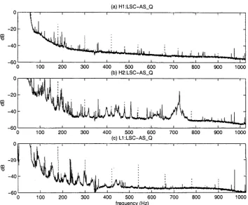
4km interferometer output power spectra (uncalibrated), be fore (dotted) and after (solid) line removal... 51 3.3 (a) Coherence of, and (b) accumulated coherence of, HLLSC-
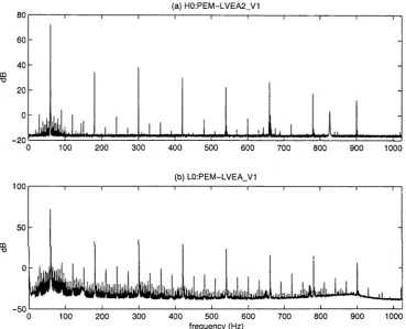
AS_Q and H2:LSC-AS_Q before (dotted) and after (solid) line removal, with the accumulated coherence of H1:LSC-AS_Q and L1:LSC-AS_Q (dashed) provided for reference... 52 3.4 (a) LHO and (b) LLO voltage monitor channel (uncalibrated)
power spectra... 53 3.5 Power spectrum of H1:LSC-AS_Q and added sinusoids before
(dotted) and after (solid) application of line removal to 300 ± 8 Hz with order 8. The power spectrum of the injected sinusoids alone is dashed. The estimation era was GPS 714974400-
714975000 and the line removal era was GPS 714975000-714975600. 60 3.6 Power spectrum of HLLSC-AS-Q and added sinusoids (dashed)
before (dotted) and after (solid) application of line removal to 308 ± 8 Hz with order 8. The estimation era was GPS 714974400-714975000 and the line removal era was GPS 714975000- 714975600. The line lies on the edge of the removal interval, and is only slightly attenuated. Other frequencies are unaffected. 62 3.7 Power spectrum of H1:LSC-AS_Q and added sinusoids (dashed)
before (dotted) and after (solid) application of line removal to 309 ± 8 Hz with order 8. The estimation era was GPS 714974400-714975000 and the line removal era was GPS 714975000- 714975600. The line lies outside the removal interval. No frequencies are significantly affected...63
LIST OF FIGURES
3.8 Power spectrum of H1:LSC-AS_Q before (dotted) and after (solid) application of line removal to 309 ± 8 Hz with order 8. The estimation era was GPS 714974400-714975000 and the line removal era was GPS 714975000-714975600... 64 3.9 Power spectrum of H1:LSC-AS_Q before (dotted) and after
(solid) application of line removal to 300 ± 64 Hz with order 8. The estimation era was GPS 714974400-714975000 and the line removal era was GPS 714975000-714975600. The line is partially removed; note the noise floor has been perturbed. . . 66 3.10 Power spectrum of H1:LSC-AS_Q before (dotted) and after
(solid) application of line removal to 300 ± 6 4 Hz with order 8. The estimation era was GPS 714974400-714975000 and the line removal era was GPS 714975000-714975600. The algo rithm has introduced noise across its band of operation... 67
3.11 Power spectrum of H1:LSC-AS_Q before (dotted) and after (solid) application of line removal to 300 ± 8 Hz with order 1. The estimation era was GPS 714974400-714975000 and the line removal era was GPS 714975000-714975600. The line has been removed to the noise floor; there is little evidence of broadening of the signal... 68 3.12 Power spectrum of H1:LSC-AS_Q before (dotted) and after
(solid) application of line removal to 300 ± 8 Hz w ith order 128. The estimation era was GPS 714974400-714975000 and the line removal era was GPS 714975000-714975600. Note perturbation of the noise floor throughout the line removal band... 69 3.13 Power spectrum of H1:LSC-AS_Q before (dotted) and after
(solid) application of line removal to 300 ± 8 Hz with order 8. The estimation era was GPS 714974996-7149750(00 and the line removal era was GPS 714975000-714975600. Note perturbation of the noise floor throughout the line removal band... 70 3.14 Coherence of (a) H1:LSC-AS_Q. (b) H2:LSC-AS_Q and (c)
L1:LSC-AS_Q with their respective voltage monitor channels. H0:PEM-LVEA2_V 1 and L0:PEM-LVEA_V1. before (dotted) and after (solid) application of the line removal technique de
LIST OF FIGURES xiii
3.15 Power spectra of the prediction for (a) H1:LSC-AS_Q, (b) H2:LSC-AS_Q and (c) L1:LSC-AS_Q (solid). Corresponding power spectra of the channels are provided for reference (dotted). 73
3.16 H1-H2 coherence with (red) and without (blue) the line re moval stage of the stochastic pipeline... 75
3.17 Per-data-segment (x ) and total (horizontal lines) upper limit results with and without line removal, showing no significant differences. The dashed lines are 90% confidence bounds on the (solid line) lim it... 76
3.18 The power spectrum of the injected line (red) compared to that of the 4 km Hanford interferometer (blue)... 77
3.19 Structural comparison of the search’s optimal filter (top) and Hi and H2 spectra (bottom), showing th at deep notches in the filter correspond to spectral lines... 78
4.1 Antenna p attern (F2 4- F 2)(0,(p) of an ideal interferometric gravitational wave detector with arms ex = x and ey = y. . . . 86
4.2 Antenna patterns of existing detectors (a) LIGO Hanford (both instruments), (b) LIGO Livingston, (c) VIRGO, (d) GEO, (e) TAMA and proposed detector (f) AIGO...89
5.1 Relative merit of an additional site to augment the LIGO Liv ingston Observatory in a coincident analysis (lighter is better, contours every 2.5%). The minimum detection rate is 41% of the maxim um ... 101
5.2 Relative merit of an additional site to augment the LIGO Liv ingston Observatory in a coherent analysis (lighter is better, contours every 2.5%). The minimum detection rate is 89% of tie maxim um ... 102
5.3 Relative merit of an additional site to augment a network con- s.sting of the LIGO Hanford (4km) Observatory, the LIGO Livingston Observatory and a 4km LIGO I instrum ent at the VIRGO site, in a coincident analysis (lighter is better, con c u rs every 2.5%). The minimum detection rate is 69% of the
XIV
LIST OF FIGURES
5.4 Relative merit of an additional site to augment a network con
sisting of the LIGO Hanford (4km) Observatory, the LIGO
Livingston Observatory and a 4km LIGO I instrument at the
VIRGO site, in a coherent analysis (lighter is better, contours
every 2.59c). The minimum detection rate is 94% of the max
imum... 104
6.1 Sidereally-averaged response to a uniform distribution of pul
sars of interferometers with varying latitudes and orientations—
effectively the familiar peanut antenna pattern averaged over a
rotation. The responses are independent of longitude; the ver
tical axis of the diagram is the Earth’s axis of rotation. From
left to right, latitudes of 0°, ±30°, ±60° and ±90°. From top
to bottom, orientations of 0, | and | from north. Note that
for the equatorial detector with a y orientation, an antenna
pattern null aligns with the Earth's axis of rotation so that no
sources from that direction could be detected...I ll
6.2 Model for the distribution of galactic pulsars, in celestial co
ordinates... 113
6.3 Detectable fraction (vertical) of a galactic pulsar population
L ist o f L istin g s
2.1 Example LDAS jo b ... 12
2.2 Universal D ata Type class definition... 16
2.3 UDT cast definition... 17
2.4 An impossible Scalar d efin itio n ... 19
2.5 Scalar<T> definition... 19
2.6 Scalar<T> conversions... 20
2.7 Sequence<T> definition... 21
2.8 Sequence<double> functionality... 22
2.9 M atrix<T> definition... 22
2.10 M atrix arithm etic operation... 23
2.11 M atrix proxy class ... 23
2.12 M atrix functionality... 24
2.13 M atrix functionality... 24
2.14 State class d e f in itio n ... 25
2.15 M ixerState class d e fin itio n ... 27
2.16 Mixer class d e f in itio n ... 27
2.17 template method Mixer::apply d e fin itio n ... 28
2.18 UDT method M ix er::ap p ly ... 29
2.19 Helper tem plate method Mixer::applyAs... 29
2.20 LinFilt class d e fin itio n ... 32
2.21 LinFiltState class d e fin itio n ... 32
2.22 Resample class definition... 34
2.23 ResampleState class definition... 35
2.24 Valid d ata conditioning API commands... 36
2.25 CallChain class definition... 37
2.26 CallChain::Function definition...38
2.27 MixFunction class definition... 38
2.28 Mix action evaluator... 39
xvi LIST OF LISTINGS
2.29 Mixer class unit te st... 41
2.30 Mix action (MixFunction class) unit t e s t ...42
2.31 LDAS mixing test jo b ...44
4.1 Compute the response matrix of a gravitational wave detector. 87 4.2 Compute the polarisation basis of a source... 88
4.3 Compute the response of a detector to a given strain... 88
4.4 Compute the response of a real observatory...90
A .l BandSelector class definition... 121
A.2 OEModel interface...124
A.3 OEModel interface (continued)...125
A.4 OEModel interface (continued)...125
A.5 OEModel interface (continued)...126
A.6 OEModel interface (continued)...126
A.7 OEModel interface (continued)...127
A.8 OEModel interface (continued)...127
A.9 OEModel state abstraction... 127
A. 10 OEModel state im plementation... 128
A. 11 OEModel state implementation (continued)...129
A. 12 Progressive model estim ator... 129
A. 13 OEModel linear filter implementation... 130
A. 14 LineRemover interface...131
A. 15 LineRemover im plementation... 134
C h a p te r 1
I n tr o d u c tio n
I f you need to use statistics, you ought to have done a better experiment.
— Lord Rutherford
If only it was that simple. Hundreds of millions of dollars have been poured
into the construction of phenomenally sensitive laser interferometers, kilo
metres long, pushing forward the state of the art in a number of fields and
breaking a litany of world records. Yet even with some of the most sensitive
instruments ever built, the gravitational waves we expect to receive will still
be at the very margins of detectability. Though sensitivities will improve,
the vast bulk of signals will remain in this marginal regime for the foreseeable
future. We cannot merely do a better experiment.
This leaves us with a need to use statistics. With the interferometers
orders of magnitude more sensitive to things as diverse as the alternat
ing current electrical supply, the moon, artillery exercises and tree-felling,
than to the infinitesimal gravitational waves emitted by colliding black holes
in nearby galaxies, the potential for false positives is immense—and unaf
fordable for a field whose very history begins with unsupportable claims.
The leading US-based Laser Interferometer Gravitational wave Observatory
(LIGO) has gone to the extraordinary length of building two vast twin in
struments at opposite corners of the continental United States, so that each
may independently validate any detection by the other. The raw output
of the instruments must be carefully vetoed, conditioned, filtered and com
pared to efficiently detect a signal—and all with a thorough understanding
of how these many processes affect the statistics of, and our confidence in,
the detection. Even with such extraordinary precautions, it is possible that
2 C H APTER 1. IN TRO D U C TIO N
there may be no single, widely agreed-upon moment of discovery—only a growing confidence, perhaps analogous to the recent process of discovery of extra-solar planets.
In this context, this thesis addresses several issues involved in improving the sensitivity of, and confidence in, the results of the emerging field of grav itational wave astronomy. The first is the author's contribution to the LIGO D ata Analysis System (LDAS), including the design, implementation, and— most im portantly—validation of primitive signal processing operations that will condition much of LIGO’s d ata output. The second is the development and—critically—characterisation of a specific data conditioning technique to remove spectral line interference. The third consists of the development of models of the collective sensitivity of a global collaboration of gravitational wave detectors, to determine the sensitivities of existing and future configu rations to a variety of possible sources, and to develop recommendations as to the configuration and expansion of the network. In the latter, the possible contribution of an Australian gravitational wave observatory is given special consideration.
1.1
R e v ie w
In the ‘weak-field lim it’ of general relativity where only small perturbations hßU to the metric of flat space-time rjßL, = diag( —1.1,1,1) are considered, the Einstein equations can be linearised. If we choose to work in the transverse traceless gauge, where the coordinate system is defined by the trajectories of freely-falling test particles, the linearisation produces a wave equation,
(
v
2-?SK=°-
(u)
representing a plane wave of space-time curvature propagating at the speed of light c.
The scale of gravitational waves can be estimated by considering the field equation T = in analogy with Hooke's law P — Eh. The ‘stiffness'
4
1.1. REVIEW
3
Only a literally astronomical expenditure of energy can produce a detectable
gravitational wave.
Until relatively recently, debate raged about the physical reality of grav
itational waves, as to whether any experiment could actually detect them.
Any such experiment would be embedded in space-time, and from the def
inition of the transverse traceless gauge used to formulate the problem, the
passage of a wave will not alter the coordinates of any test particle in the
experiment. However, it is not the coordinates of test particles but rather
the measured distance
j yjg^dx^dx1'
between two freely falling particles
that will be changed as the space-time metric
g
A
i£, =
4-
hßU
is perturbed.
Gravitational wave detection consists of making this measurement.
The first generation of gravitational wave observatories were
resonant
mass detectors
, or
Webber bars.
Webber noted that a gravitational wave
passing through a solid body would change its length, and if the body was
resonant with the gravitational wave, each cycle would coherently add until
a detectable amplitude resulted. Although Webber's claims to have observed
gravitational radiation are discredited, over the intervening decades Webber
bars have grown in size, sophistication and sensitivity—now approaching the
10-21 level in narrow frequency bands—but they have not yet made any
detections.
The current generation of gravitational wave detectors is very different:
based, in a pleasing piece of historical serendipity, on the Michelson interfer
ometer, whose disproval of an aether drift was one of the cornerstone pieces
of experimental evidence for relativity.
A Michelson interferometer consists of a light source (in modern instru
ments, a coherent laser light source), a beam-splitter and two mirrors. Light
enters the beam-splitter, and is split into two beams. Each beam travels
down an ‘arm' of the interferometer, is reflected by an end mirror back to
the beam-splitter. The beam-splitter recombines the returning coherent light,
producing interference fringes. These fringes depend sensitively on the dif
ference in the lengths of the two arms—to a fraction of a wavelength of the
light—making the Michelson interferometer a sensitive measure of distance.
4
CHAPTER 1. INTRODUCTION
be ‘folded7 by adding an additional mirror in each arm to reflect the light
back and forth in the arm for either a fixed (delay line) or statistical (optical
cavity) amount of time, reducing the current generation of interferometers
to more manageable—but still challenging—arm lengths of a few kilometres.
The limiting factors on such a large and sensitive instrument range from
the profound (numerous quantum effects such as the uncertainty in the po
sition of the mirrors) to the absurd (seismic noise from road bumps), and
every attempt is made to limit their effect.
However, once the signal from the output photodetector has been digitised
and recorded, the problem of gravitational wave detection shifts from one of
engineering and experimental physics to the nascent field of data analysis.
The hard-won output of gravitational wave detectors must be scrubbed of
any remaining identifiable noise sources, and scoured for the faintest of grav
itational wave signals. This thesis addresses the problems of how to remove a
particular class of environmentally correlated noise from the output of grav
itational wave detectors, and, looking to the future, examines how best to
combine the output of detectors around the globe as the field moves from
gravitational wave detection to gravitational wave astronomy.
1.2
P u b l i c a t i o n s
Much of the work in this thesis relates to previous publications of its author.
Specifically, Chapter 3 expands upon (2, 4 and 14). and Chapters 4, 5 and
6 expand upon (3). (1. 5. 6. 8 and 9) contain information on the Australian
gravitational wave effort, and in particular the local establishment of a LIGO
Data Analysis System (LDAS) as described in Chapter 2. I am honoured to
have participated in the analysis for, and to be one of the many authors of,
the first LIGO observational results (7 and 10-14).
1. D McClelland. S Scott, M Gray, D Shaddock, B Slagmolen, A Searle,
D Blair, J Lu, J Winterflood, F Benabid, M Baker, ,1 Munch, P
Veitch, M Hamilton, M Ostermeyer, D Mudge. D Ottaway, C Hollitt.
“Second-generation laser interferometry for gravitational wave detec
tion: ACIGA progress",
Class. Quant Grav.
18 4121-4126 (2001).
1.2. PU BLICATIO NS 5
Grossmann Meet. Gen. Rel. (eds. V Gurzadyan, R Jantzen, R Ruffini), World Scientific Singapore, 1919-1920 (2002).
3. A Searle, S Scott and D McClelland, “Network sensitivity to geo graphical configuration” , Class. Quant Grav. 19 1465-1470 (2002).
4. A Searle, S Scott and D McClelland, “Spectral Line Removal in the LIGO D ata Analysis System (LDAS)” , Class. Quant Grav. 20 S721- S730 (2003)
5. J Jacob et al, “A ustralia’s Role in Gravitational Wave Detection” , Pub. Astro. Soc. Aust. 20 223-241 (2003)
6. M Gray et al, “ACIGA: Status R eport” , Proc. SPIE (Gravitational- Wave Detection; eds. M Cruise, P Saulson) 4856 258-269 (2003)
7. B Allen et al, “Upper limits on the strength of periodic gravitational waves from PSR J 1939+2134” , Class. Quant Grav. 21 S671-S676
(2004)
8. S Scott, A Searle. B Cusack and D McClelland, “The ACIGA Data Analysis Programme” , Class. Quant Grav. 21 S853-S856 (2004) 9. L Ju et al, “ACIGA's high optical power test facility” , Class. Quant
Grav. 21 S887-S893 (2004)
10. B A bbott et al, “Detector Description and Performance for the First Coincidence Observations Between LIGO and GEO", Nuc. Inst. .4
517, 154-179 (2004)
11. B A bbott et al, “Setting upper limits on the strength of periodic gravi tational waves from PSR J1939+2134 using the first science d ata from the GEO 600 and LIGO detectors", Phys. Rev. D 69. 082004 (2004) 12. B Abbott et al, “First upper limits from LIGO on gravitational wave
bursts” , Phys. Rev. D 69, 102001 (2004)
13. B A bbott et al. “Analysis of LIGO data for gravitational waves from binary neutron stars", Phys. Rev. D 69. 122001 (2004)
6
CHAPTER 1. INTRODUCTION
1.3
O v e r v ie w
Part I deals with the software infrastructure for the analysis of LIGO data
throughout this decade. Chapter 2 gives an overview of the LIGO Data
Analysis System (LDAS) and details the implementation and validation of
the basic elements of the
data conditioning A PL
including its primitive signal
processing operations. Chapter 3 considers the development of a data condi
tioning tool to remove spectral line interference: its implementation within
the data conditioning API using the functionality of Chapter 2, validation of
its correctness, and characterisation of its ability to improve the recovery of
gravitational wave signals.
P a r t I
D a ta C o n d itio n in g
C h a p te r 2
T h e L D A S d a t a c o n d itio n in g
A P I
Shouldn't acronyms be expanded in titles?
— Katie Weir
The light amplification by stimulated emission of radiation interferometer gravitational-wave observatory data analysis system data conditioning appli cation procramming interface?
— Antony Searle
This chapter is intended to serve a dual purpose: first, to familiarise the reader wit.r the elements of the data conditioning API utilised by the im plementation of the line removal technique in C hapter 3; second, to provide a guide to the 'design and evolution’ of the d ata conditioning API for its future m ahtainers and contributors. The elements referred to in Chapter 3 are largely among those to which the author made substantial contributions, and, happly, are illustrative of the system as a whole.
We begin with a brief survey of LDAS, noting in particular the posi tion and finction of the data conditioning API within it. followed by a dis cussion of the motivating factors behind the d ata conditioning API itself. The devekpment has proceeded in parallel with the commissioning of the LIGO instillments, meeting milestones to facilitate engineering and science 'runs’, incliding 'Mock D ata Challenges’ (MDCs) consisting of integration and stress esting.
10 C H APTER 2. THE LDAS DATA CONDITIONING A P I
The code listings presented in this chapter have been edited (often ex tensively) for clarity. Unless otherwise noted, the original code is publicly available from the LDAS repository [lj. Brief notes on the C + + language have been included in the text as an aid to interpreting the listings; for an authoritative introduction to the C + + language, we recommend [2],
D isclaim er The author is a significant, but not the sole or even primary contributor to the d ata conditioning API, which is a collaborative effort be tween many contributors from LSC institutions, coordinated by the Califor nia Institute of Technology.
2.1
T h e L IG O D a ta A n aly sis S y stem (LD A S)
To search for gravitational wave signals in noisy data optimally (in the theo retical sense) is, in general, computationally expensive. In practice, approx imately optimal methods are used; their sensitivity is limited by available computational cycles, memory or network bandwidth. As the instruments continuously acquire data, this processing must occur in real time, or an unmanageable backlog will result.
The need for continuous real-time computation ruled out the use of gen eral purpose supercomputing resources. Instead LIGO elected to develop a custom system to run on its own hardware.
An LDAS implementation runs on a heterogeneous network of Sun or x86 Linux servers coupled to a Beowulf cluster of inexpensive commodity PCs. LDAS is responsible for acquiring on the order of a terabyte of information from the observatories daily and caching it locally, producing a reduced data set (RDS) for transfer to an archive and other LDAS implementations, and pre-processing the data and managing the specific parallel codes th at search the data for gravitational wave signals.
2.1. THE LIGO DATA ANALYSIS SYSTEM (LDAS)
2.1.1
A P Is
11
LDAS software is implemented as a number of Application Programming In
terface (API) libraries of compiled C++ code, which are called by interpreted
TCL (Tool Command Language [3]) script drivers. The term ‘API’ has also
come to refer to the process relying primarily on a particular API library.
Each API typically resides on a different machine; they communicate with
each other over a network.
LDAS jobs are typically configured as a ‘pipeline’. Data is read into the
system by one API, then passed along to another that processes it and passes
it along to another API.
The
manager
API oversees the LDAS system. It receives incoming user
commands and passes them on to the relevant API. It is responsible for start
ing and stopping the other APIs and regularly polls their state, restarting
any that have crashed or become unresponsive.
The
disk cache
API maintains a list of the data files available to the LDAS
system.
The
frame
API responds to queries for data specified by time and channel,
and queries the disk cache API for the pertinent files. It then reads the files
to extract segments of the channels, concatenates the data together, and, if
necessary, converts the data to the requested sampling rate, before passing
it on.
The
data conditioning
API processes data received from the frame API
before passing it on to the wrapper API (or another target). It uses a flex
ible command language to apply a broad range of built-in signal-processing
actions.
The
wrapper
API manages the parallel search codes, providing a 'wrap
per’ around an off-the-shelf implementation of the Message Passing Interface
(MPI) [4] standard for parallel computation. It provides assistance for the
common tasks of input, output and load-balancing.
(There are other APIs—most notably the database-wrapping
metadata
API—that do not concern us at this time.)
2 .1 .2
C o m m a n d la n g u a g e
12
CHAPTER 2. THE LDAS DATA CONDITIONING API
authentication purposes (the manager API maintains its own structure of user accounts and permissions), and the email address of the user, to which a message containing (the URL to) the results of the job (or a diagnostic mes sage) are sent. Often, the 'user' is in fact a driver program. (Jobs are often w ritten as TCL scripts; when executed they can substitute in values derived from arguments or environment variables and then submit themselves.)
Listing 2.1: Example LDAS job.
IdasJob {
— name acsearle — password ******* —email acsearle@localhost
}{
dataPipeline —framequery {
{ R H {} 714975000-714975001 Adc(Hl:LSC-AS_Q!resample!8!) }
}
—output { ilwd ascii } —aliases { h 1 = HI; }
—datacondtarget { datacond } — algorithms {
x = slice(hl, 0, 1024, 1); # data, start, count, stride output(x,_,x,x,x);
}
The type of job (in this case, dataPipeline) dictates which named options are required.
The —framequery option lists the data th at will be required by the job. (The data type is R, Taw', and the observatory is H. Hanford.) Xo files, {}, are specified; these will be automatically determined by the frame API. The ‘era' requested is the 1 second interval between GPS times 714975000- 714975001. The frame API will seek the Adc (analog-to-digital) channel named H1:LSC-AS_Q (the output of the 4 km interferometer); the postfix
!resample!8! instructs the frame API to downsample the channel by a factor of 8 (in the case of HLLSC —AS_Q. from 16384 Hz to 2048 Hz).
2.2. DESIGN AND EVOLUTION 13
The target for the output of the d ata conditioning API is the data con ditioning API itself, -datacondtarget { datacond }, which causes its output to be w ritten to disk. (To conduct searches the output would be sent to the w rapper API.)
The -o u tp u t format will be ilwd ascii, a human-readable (ASCII-encoded) version of the XML-derivative Internal LightWeight D ata (ILWD) format used by LIGO.
The —algorithms option is where the d ata conditioning API command language is embedded. It consists of a series of C- or MATLAB-like statem ents forming a fully programmable signal-processing pipeline. (In this case, it slices off the first 1024 elements of the input d ata into the variable x and outputs it.) It is the implementation of this functionality th at will concern us for the rest of this chapter.
2 .2
D e s ig n a n d e v o lu tio n
The original design for the d ata conditioning API is encapsulated in [5]. The seeds are to be found there of the issues th at would come to dominate its development.
The data conditioning API library is written in ISO C + + . The rationale given in [5] mentions its C heritage, the (then recent) ANSI/ISO standardi sation of the language, and the benefits of its object-oriented features. The prim ary motivation is one of efficiency: C + + is a compiled language, with m ature optimisers, and typically runs faster and uses less memory than inter preted languages. Moreover, it permits higher-level abstractions (and thus has better prospects for reuse and maintenance) than C while maintaining, bv design, ’95%! of C's performance; this is a consequence of (its designer) S tro u stru p ;s “you don't pay for what you don't use” philosophy [2] and was perhaps the leading factor in its widespread adoption. (Counter-intuitively, the combination of C + + ’s template and inline features can produce code th a t is faster than C, by shifting some computation from run-tim e to compile tim e [6].)
Though the standardisation of C + + represented a great step forward, the standard itself differed significantly from existing practice.1 Some use ful and significant parts of the standard proved pathologically difficult for
14
CHAPTER 2. THE LDAS DATA CONDITIONING API
vendors to implement. It was not until late 2002 th at a compiler was finally released th at could reasonably claim compliance to the standard; the difficul ties experienced by its implementers have been held up as reason to amend certain features in the next iteration of the standard (the C + +-0x standard, expected sometime in the middle of this decade). Throughout the period of development discussed here (2000-2003 inclusive) the GNU C + + com piler used by LDAS has improved dramatically, but much of the code base has been impaired by this shifting foundation. (Perhaps the most obvious sign of this is the persistence of the once-necessary evil of explicit template
instantiations.2)
Compounding the problem of a changing language implementation, the C ++-97 standard also spawned a change in the C + + programming idiom. Meyers laments in his foreword to Alexandrescu [7] th at the C + + commu nity’s understanding of templates has been undergoing ‘'dramatic change” for a decade. Similar changes in thinking on exception specifications and other features have also occurred. These new features and idioms could have been helpful in the design and implementation of LDAS. but most were not even conceived of. let alone widely known, at that time. (Many of these techniques appear in [7] and the useful Boost library [8], some parts of which are proposed for inclusion in C++-0x.)
The LDAS model of an API as a compiled library driven by an inter preted script has several benefits. The library performs specific well-defined tasks quickly and efficiently at the cost of flexibility (in the sense of rapid development). Complementarity, the script may be rapidly altered to make use of th at functionality in different ways.
The data conditioning API inherited this two-tiered model from the de sign of LDAS as a whole, but in its particular case the model caused problems. This framework is most applicable when the functionality of the library is stable, and the interface it presents to the script is correspondingly stable, concise, and well-defined. The requirements placed on the data conditioning API meant th at these conditions were not consistent with reality. The gen erality of the operations required by the data conditioning API—effectively the implementation of a numerically-oriented programming language some what like MATLAB—caused an explosion in the number of data types3 and
2 Not, a search template!
2.2.
DESIGN AND EVOL UTION
15
operations that had to be implemented in C++ and exposed to and handled
by the scripting layer.
It was realised at the first Mock Data Challenge that this model of de
velopment was unsustainable. The first step in fixing the problem was the
rapid development of a ‘universal data type’, so that only one type needed
to be exposed to the scripting layer. It was followed by the adaptation of
existing signal-processing operations to a new call-chain framework that is
effectively a simple
virtual machine.
The involvement of the scripting layer
in the implementation of the data conditioning pipeline was reduced until it
merely parsed input (it still performs an important role in initialisation and
output).
The problem of data typing, or more specifically, the problem of how
to efficiently implement the un-typed data conditioning API command lan
guage in strongly typed C++, came to dominate the implementation, and
has not yet been adequately addressed. Development at the moment relies
at least partially on the brute-force handling of the multiplicity of combina
tions of operations and data types. This leaves the implementation with a
fundamental scalability problem.
It is not readily apparent (to the author, at least) at this time how the
original design could have been implemented in a significantly superior way.
Radical changes in the design could be supposed to fix some or all of the
problems that were encountered, but there would be no guarantee that they
would not introduce their own issues. Part of the problem is due to the well-
known issue of
multiple dispatch
(run-time polymorphic behaviour on more
than one type), an issue not addressed by C++ (or most modern languages).
The adoption of more modern C++ techniques would undoubtedly improve
conciseness and reduce repetition, but would not in itself address the fun
damental scalability issue. No such proposal has yet merited the large-scale
overhaul of what is, after all, a working code base.
It should be noted that the above discussion is in some sense an argument
over aesthetics (though it does affect the practicality of future expansion).
The problems are not apparent to the user, only the developer. In particular,
a stringent testing regimen ensures that the results produced by the data
conditioning API are correct.
16 C H A P T E R 2. THE LDAS DATA CONDITIONING API
2.3
U n iv e r s a l D a t a T y p e ( U D T )
The Frame data format of LIGO and Virgo, and the ILWD format of LDAS. support a wide range of d ata types: 8-, 16-, 32- and 64-bit integers, 32- and 64-bit floating point real numbers, and 64- and 128-bit complex numbers (composed of pairs of reals). The data conditioning API must be capable of operating on all of them, either singly (scalars) or in (homogeneous) arrays (vectors, matrices, and higher dimensional arrays). This means th at LDAS must support over a dozen types. When m etadata is considered—for ex ample, decorating a vector with information declaring it to be a time series of a particular sample rate and start time—the number of types becomes immense.
The ‘universal d ata type’, or UDT, is intended to hide all these types behind a common interface. Only those operations which need to know the exact type of a UDT will have to look beyond the interface. Much of the data conditioning API implementation can remain oblivious to the exact nature of the d ata flowing through it.
2.3.1
I m p le m e n ta tio n
The inheritance mechanism of C + + is exactly the mechanism required for the implementation of UDT. The UDT is a base class exposing those operations common to its derived classes (the data types). Each data type ‘is-a’ UDT,
as a sedan ‘is-a' car: they are said to inherit from it.
The interface of UDT is the intersection of the interfaces of all its pos sible derived classes, and is necessarily ‘thin', consisting only of creation, destruction, copying, and methods to assist in the resolution of the derived class.
Listing 2.2: Universal Data Type class definition.
class UDT
{
public:
virtual ~UDT(); / / destroy
virtual UDT* CloneQ const = 0; / / (deep) copy
template<class T > static bool lsA(const UDT& In); / / is it really
2.3. U NIVERSAL DATA T Y P E (UDT) 17
template<class T > static T & Cast(UDT& In); //a c c e s s it as a type T (or throw an exception)
/ / . . . (omitted)
};
In this listing, the first line opens the definition of class UDT. circumscribed by braces {•••}• The keyword public declares all which follows to be uni versally accessible (the default is private, meaning th at only the class imple m entation itself has access).
The class itself (in the simplified version we present) consists only of methods, and has no data members. A method is a function th at is a member of the class; its full name is prefixed with the class name, as in UDT::Clone, and it can only be invoked on an instance of UDT, as in my_udt.Clone(), in which the method receives my_udt as the implicit ‘zeroth’ argument this.
(The static keyword indicates a method th at is associated with a class, but is not invoked on an instance of th at class.)
The virtual destructor virtual ~UDT() cleanly destroys the UDT instance on which it is invoked. The virtual keyword indicates th at the method may (should) be overridden by derived classes; derived classes will replace the UDT method with a method th at can cleanly destroy the particular imple mentation of th at derived type. Even when the UDT is destroyed in a context th a t knows nothing about the derived type, the correct method will be called.
The deep copy method virtual UDT* CloneQconst = 0 makes a copy of the UDT th at is aware of the particular derived type, just as is the virtual destructor is. The method returns a pointer, UDT*, to a copy of the derived type instance created by the new operator. The const keyword indicates that the original is unaffected by the copying process. The = 0 syntax indicates th at the method may not be supplied by UDT; this makes the method pure virtual and the UDT class abstract—UDT cannot be instantiated, and derived types must override Clone. (Ideally the virtual destructor should also be pure.)
The template<class T > methods IsA and Cast are examples of generic code. Many d ata types may inherit from UDT; we cannot (and should not) write specific code to check each case. Instead we note th at the code to check a particular case differs only in the particular type for which we wish to check. The template keyword allows us to write a generic definition that works for all types by writing it in terms of the template parameter ‘T \ (The
18 C H APTER 2. THE LD AS DATA CONDITIONING A P I
Listing 2.3: UDT cast definition.
template<class T > T & UDT::Cast(UDT& a) \
{
return dynamic_cast<T&>(a); \
}
The Is A c T> method allows us to check if a UDT instance is really an instance of class T (returning a boolean true or false), and the C a st< T > method allows us to access the class T instance itself. If we attem pt to perform a bad cast—if the UDT is not a T—a bad_cast exception is thrown at runtime. This can be avoided by checking first with lsA < T > .
C r i t i q u e
The UDT as presented above is textbook object oriented programming (OOP). As such, it is open to the criticisms of C + + 's implementation of OOP. Clone's use of raw pointers is potentially dangerous: the innocuous statem ent ‘ my_udt .CIone();! is valid but results in a memory leak. The default and copy con structors should be protected (so th at only derived classes may call them) and the assignment operator explicitly left undefined as their default be haviour will make slicing (copying or assigning a more derived class to a less derived class) possible [9]. Other implementations of OOP, for example Java, already have a universal base class from which all classes are defined. C + + eschews this approach as introducing unacceptable overhead; the slicing and pointer issues arise from similar considerations.
The formulation of IsA and Cast as static methods taking a UDT argument rather than plain methods or helper functions is bizarre; however, at one time it was a necessary work-around for an equally bizarre compiler error.
A ’better' UDT would probably adopt the pomter-to-implementation (‘pim ple') idiom. The current arrangement would be wrapped by a new handle class with conventional copying semantics, eliminating the problem of the user dealing directly with slicing and pointers. The handle could be made smart [7, 10] to permit lazy copying, eliminating an issue we will encounter in §2.4.
2.3.2
S calar
repre-2.3. U NIVERSAL DATA T Y P E (UDT) 19
sented at various precisions—yet they all have the same basic requirements. We can represent this commonality using generic coding, templatising Scalar on an unknown type T.
The design of Scalar presents an interesting problem. One choice denied to us is to inherit from the unknown type T, and thus inherit its interface, so th a t an object of type Scalar<T> could be used wheresoe’er a T is expected.
Listing 2.4: An impossible Scalar definition
tem platectypenam e T> class Scalar : / / inherits from
public UDT, / / a n d
public T
{
/ / . . . (omitted)
};
We cannot do this because at least some of the types we will use will be basic, such as int and float, which are not classes and cannot be inherited from. (Making basic types full classes would impose performance overhead in common cases. Java, for example, faces the same trade-off, but makes the opposite decision.) Moreover, even for the types th at are classes (complex <f ! oat > and complex<double>) derivation is problematic as they were not intended to be used as base classes, do not have virtual destructors, and thus have the potential for undefined behaviour.
Instead we must rely on implicit and explicit conversions between Scalar < T > and the type T:
Listing 2.5: Scalar<T> definition.
template<typename T> class Scalar :
public UDT
{
public:
explicit Scalar(T); / / explicit conversion from T
virtual ~Scalar(); / / override
virtual Scalar* CloneQ const; / / override
operator T&(); / / implicit conversion to T
operator const T&() const; / / implicit conversion to const T
20 C H APTER 2. THE LDAS DATA CONDITIONING A P I
void SetValue(const T&); / / mutator
/ / . . . (omitted) private:
T m_value; / / encapsulated value
};
The constructor accepting a T defines a conversion from an instance of T to an instance of Scalar<T>. As T matches almost any type (precisely, any copy- constructible type) it is declared explicit to prevent its implicit application by the compiler in situations where the programmer did not explicitly request it. An implicit conversion such as this would allow anything to be converted into its Scalar equivalent, which ‘is-a’ UDT; this would subvert the process of compile-time error checking.
The implicit conversion to a reference to the encapsulated T instance is defined by operator T& (and its const variant; which version is called depends on the context). As it is implicit, the compiler has license to convert a Scalar<T> to a T wherever it finds it expedient to do so; most commonly where a Scalar<T> is passed as an argument to a function expecting a T.
Listing 2.6: Scalar<T> conversions.
Scalar<complex<double> > z(complex<double>( —1., 0.)); / / explicit conversion from complex to scalar
sqrt(z); / / implicit conversion from scalar to complex to use complex square root
z.realQ; / / error: ‘real’ undeclared
complex<double>(z).real(); / / conversion made explicit
Implicit conversion does not occur everywhere that we might hope; for ex ample, complex<T> defines methods real and imag that we cannot invoke on a Scalar<complex<T> > without explicitly invoking the conversion.
For this reason, we also provide traditional accessor and mutator methods to get and set the wrapped value. Note that GetValue does not change the value, and is thus const: SetValue does change the value, and is non-const.
2.3.3
S e q u e n c e
2.3. UNIVERSAL DATA TYPE (UDT)
21The basic C++ sequence type is the array. Inherited from C, it is an
inconvenient and perilous language construct. The C ++ Standard Tem
plate Library (STL) supplies a wide range of container types to replace it;
its
valarray<T> [2]is targeted at numerical computation. The C++ stan
dard allows implementers unusual latitude in the
valarray<T>specification
to facilitate the implementation of aggressive optimisation. It provides fast
vector arithmetic and BLAS (Basic Linear Algebra Subprograms)-like [11]
subsequences.
As
valarray<T>is a class, we may inherit from it as well as
UDTwhen
we design
Sequence<T>,an option which we had to reject for
Scalar<T>.(Note that
valarray<T>does not include a virtual destructor, so unfortu
nately there is the potential for undefined behaviour in the unlikely event
of a user destroying a
Sequence<T>as a
valarray<T>.)This way,
Sequence < T >automatically inherits most of
valarray<T>’sinterface, such as the
subscript
operator[]’ and the
sizemethod. (Unlike many
OOPlanguages
C + + supports inheritance from multiple base classes.)
Listing 2.7:
Sequence<T>definition.
template ctypename T>class Sequence : public UDT,
public valarray<T> {
public:
Sequence(size_t n); / /
construct with n (default) elements
Sequence(const T& x, size_t n); / /
construct with n copies of x
Sequence(const valarray<T>&:); / /
implicit conversion from valarray
virtual ~Sequence(); / /
override
virtual Sequence* CloneQ const; / /
override
/ / ...
(omitted)
};
22
CHAPTER 2. THE LDAS DATA CONDITIONING API
The inherited functionality allows us to invoke all the methods of
valarray <T>on
Sequence<T>:Listing 2.8:
Sequence<double>functionality.
Sequence<double> a(3); / / asequence of 3 elements
a[a.size() — 1] = 1.0; / /
set the last element
2.3.4
M a tr ix
There is no type in the STL representing an
nx
mmatrix; we follow the
suggestion in Stroustrup
[2]and implement a generic
Matrix<T>class using
a packed
valarray<T>of
nmelements.
Listing 2.9: Matrix<T> definition.
template<class T>class Matrix :
public UDT
{
public:
Matrix(size_t rows, size_t columns); / /
rows— by—columns matrix
virtual “MatrixQ; / /
override
virtual Matrix* CloneQ const; / /
override
size_t rows() const; / /
accessor
size_t columnsQ const; / /
accessor
/ / . . .
(omitted)
private:
valarray<T> m.data; / /
representation
size_t m_rows; / /
dimensions
size_t m_columns;
};
Internally the representation is straightforward: two
size_ts(non-negative in
tegers) represent the dimensions
nand
mof the matrix; the elements are
packed into a
valarray<T>(the packing is
Fortran-rather than C-ordered
to facilitate the use of
C Lapack (12]).The dimensions are set on construc
tion and may be checked with the
rows()and
columnsQaccessors.
2.3. UNIVERSAL DATA TYPE (UDT)
23
Listing 2.10: Matrix arithmetic operation.
Matrix&operator+=(const
Matrix& right){
/ / ...
(check dimensions)
m.data + = right.m_data; / /
use valarray +=
return *this;
/ /self—reference
}
/ / ...
(arithmetic operators)
To support C++-style subscripting of a
Matrix<T>instance, as in
A[i][j],we must implement an
operator[]
method. This is not a trivial undertaking,
as
operator[]
must return a
proxy object
representing a row (or column) of
the
Matr ix<T>,with its own
operator]]
that finally returns a reference to
a
Matr ix<T>element. The STL class
slice_array<T>,a proxy object for
sub-array slices of
valarray<T>,is almost ideal for our purposes, but unfor
tunately its copy-constructor is private, preventing any methods but those
of its
friend
valarray<T>from returning it. Instead we implement member
class
Matrix<T>:: proxy .array,with essentially the same interface as
slice_array < T > ,leveraging
slice_array<T>internally, to access rows and columns of the
matrix. The
sliceclass (another
valarray<T>helper class) stores the start
index, stride, and number of elements of the array slice.
Listing 2.11: Matrix proxy class
1
class
proxy_array{
friend class
Matrix<T>;public:
operator const
valarray<T>()const;
/ /conversion
proxy_array&
operator=(const
valarray<T>&); / /assignment
T&
operator]]
(size_t); / /subscripting
const
Toperator[](size_t
i)const;
/ /const subscripting
proxy_array&
operator-h=(const
valarray<T>& right); / /arithmetic
/ / ...
(arithmetic operators)
private:
valarray<T>& m_data; / /
reference to matrix elements
slice m_slice;
/ / subarray parameters
};
proxy_array row(size_t); / /
reference a row
24 C H APTER 2. THE ID A S DATA CONDITIONING A P I
proxy .array column(size_t); / / reference a column
const proxy .array column(size.t) const;
proxy .array operator]] (size.t); / / synonym for row
const proxy .array operator]] (size.t) const
The proxy .array forwards assignment and arithm etic operations to the indi vidual elements of the matrix. The m utators row, column and operator]] all return proxy.arrays referencing the corresponding subset of the matrix; the proxy.array itself behaves like a valarray<T> whose elements are embedded in the Matrix<T>. Users will typically never see the proxy.array.
Listing 2.12: Matrix functionality. Matrix<double> A(3, 3); / / 3x3 matrix
A[l] = 1. ; / / centre row set to [1 1 1]
A[l][1] = 0.; / / centre element set to 0
A number of non-member operators are also supplied for Matrix<T>.
Listing 2.13: Matrix functionality.
tem platectypenam e T > Matrix<T> operator+(const Matrix<T>& left, const Matrix<T>& right)
{
return Matrix<T>(left) + = right; / / add to a copy and return that }
/ / (...) arithmetic operators
Higher-dimensional arrays have not yet been required (at the interface level) in the data conditioning API.
2.3.5
M e ta d a ta
Many of the series used in the data conditioning API are time series; m eta data about these series, like their sampling rate and start time (from which the sample times can be computed) are useful in many contexts. In the case of a Fourier transform, the time series m etadata can be used to calibrate the frequency resolution of the transformed series, which can then be stored as frequency series metadata.