Problems in prediction

P ro b le m s in P r e d ic tio n

A n d re w J a m e s R ieck

November, 2001

A thesis submitted for the degree of Doctor of Philosophy of The Australian National University.

© Andrew James Rieck 2001

All rights reserved. This work may be reproduced in whole or in part, by any means possible, without the permission of the author,

D e c la ra tio n

This thesis emanates from Andrew Rieck’s research only, with all other material explicitly refer­ enced. Andrew Rieck declares that the results contained in this thesis have not been submitted for any other degree.

A c k n o w le d g e m e n ts

As for any project, I am grateful to those people who provided moral and technical support during this undertaking. Special and deeply personal thanks go to J. T., A. J., A. P., C. N., P. F., M. M., P. M., and my supervisor, Professor Peter G. Hall.

A b s tr a c t

The role of predictive inference is to provide indicative information about a predictand. Typically, this takes the form of a predictor or a prediction region. While the former provides an unambiguous point specification for the predictand, the latter can be perceived to be more informative since its construction is conjoined with prior probability assignment for the predictand.

This thesis defines and reviews the construction and properties of prediction regions. Paramet­ ric and nonparametric populations are considered. Methods used to construct prediction regions with identical canonical form are predominantly assessed via coverage error properties.

For a nonparametric population, methods used to construct prediction intervals are suggested for reducing coverage error. The jackknife and smoothed bootstrap are investigated for calibration of prediction intervals; the jackknife performs poorly in that it increases coverage error by an order of magnitude, while the smoothed bootstrap is successful at further reducing coverage error.

C o n te n ts

D e c la r a tio n

A c k n o w le d g e m e n ts

A b s tr a c t in

1 I n tr o d u c tio n

2 P a r a m e tr ic A p p r o a c h e s

2.1 Pivotal T ran sfo rm atio n s... 2.2 Predictive Likelihood... 2.2.1 Sufficiency Based Predictive Likelihood 2.2.2 Approximate Predictive Likelihood . . . 2.3 Predictive F u n c tio n s ... 2.4 Predictive Densities ... 2.5 Coverage Error and C alib ra tio n ...

3 N o n p a r a m e tr ic A p p r o a c h e s

3.1 Independent and Identically Distributed Sample 3.1.1 Studentised M e t h o d ... 3.1.2 Quantile Estimation M e th o d s... 3.1.3 Predictand S t a t i s t i c ... 3.2 Regression and Structural M odels...

4 N o n p a r a m e tr ic P r e d ic t io n I n te r v a ls

6 10 16 16 22 24 26 34

45 45 49 51 58 60

C o n te n ts v

4.1.1 One Order Statistic ... 68

4.1.2 Interpolation among Two Order S ta tis tic s ... 69

4.1.3 Interpolation among Three Order S ta tis tic s ... 70

4.1.4 Interpolation among Four Order S ta tistic s... 74

4.2 Prediction Interval C a lib r a tio n ... 76

4.2.1 Failed Jackknife C alibration... 77

4.2.2 Smoothed Bootstrap C a lib ra tio n ... 79

4.3 Theoretical P r o p e r tie s ... 82

4.3.1 Statement and Proof of Theorem 4 . 1 ... 82

4.3.2 Statement and Proof of Theorem 4 . 2 ... 93

4.3.3 Statement and Proof of Theorem 4 . 3 ... 99

4.3.4 Statement and Proof of Theorem 4 . 4 ... 103

5 N u m e r ic a l E v a lu a tio n a n d P r o p e r tie s o f P r e d ic t io n I n te r v a ls 123 5.1 Coverage Error A p p ro x im a tio n ... 124

5.2 Approximation of Additive Tuner E s tim a to r s ... 125

5.3 Numerical P ro p e rtie s... 129

A T a b le s 139

L ist o f F ig u re s

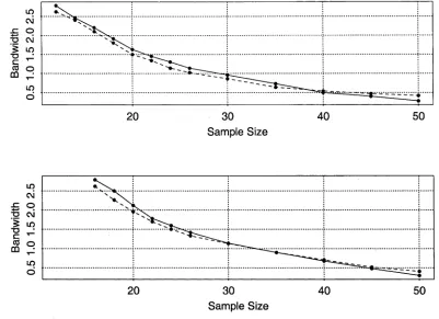
5.1 Optimal Bandwidths. Plotted are bandwidth values that minimise absolute coverage error for a standard normal population, various values of sample size, n, and nominal coverages a — 0.9 and 0.95 for the former and latter plot, respectively. Bandwidths ^N,Q2,a (dashed line) and /iN,Q3,a (solid line) are appropriate for prediction intervals ^ac,Q2,q and Xac,Q3,q, respectively... 130 5.2 Coverage Errors. Values of coverage error for prediction interval Zq i)Q, when the

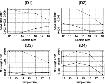
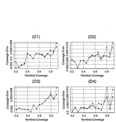
population model P is given by D l, D2, D3, and D4, the sample size n is given by 12, 14, 16, and 18, and nominal coverage a = 0.9... 133 5.3 Coverage Errors. Values of coverage error for prediction interval Xq2,q (dashed line)

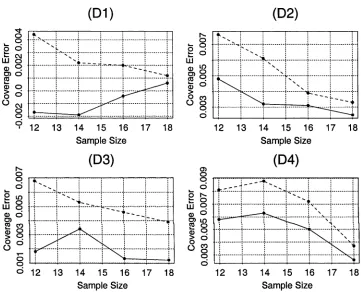
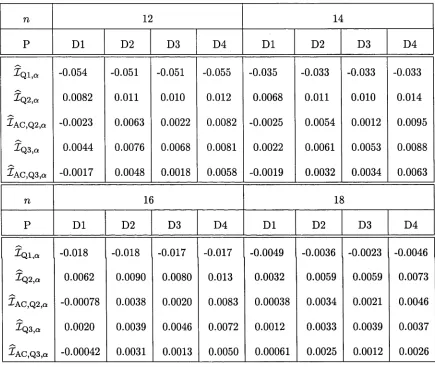
and Xac,Q2,q (solid line), when the population model P is given by D l, D2, D3, and D4, the sample size n is given by 12, 14, 16, and 18, and nominal coverage a = 0.9. 134 5.4 Coverage Errors. Values of coverage error for prediction interval Xq3)Q (dashed line)

and Zac,Q3,q (s°lid line), when the population model P is given by D l, D2, D3, and

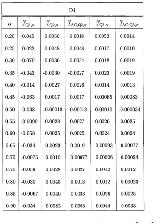
D4, the sample size n is given by 12, 14, 16, and 18, and nominal coverage a = 0.9. 135 5.5 Coverage Errors. Values of coverage error for prediction interval Xql a when the

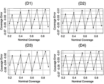
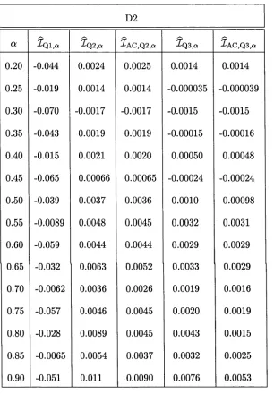
population model P is given by D l, D2, D3, and D4, and the sample size n = 12, for various values of nominal coverage... 136 5.6 Coverage Errors. Values of coverage error for prediction intervals Zq2,q (dashed line)

and ZAc,Q2,a (s°lid line), when the population model P is given by D l, D2, D3, and D4, and the sample size n = 12, for various values of nominal coverage... 137 5.7 Coverage Errors. Values of coverage error for prediction intervals Xq3)Q (dashed line)

and 2^ac,Q3,q (solid line), when the population model P is given by D l, D2, D3, and

C hapter 1

In trod u ction

The probability distribution function is a fundamental concept in statistics. If X is an

m-dimensional random vector on a probability space (Q ,P, P), its probability distribution function

F (Chow and Teicher, 1997, Section 6.3) allows probabilities associated with X to be found from the relationship

P ( X £ A) = J l A(x)dF(x)

for any A G P m, the class of m-dimensional Borel sets, where x G Mm and

Ia(z) =

for x 0 A,

for x G A.

Therefore knowledge of the function F allows the construction of a region, denoted by P Q, such that P { X G 7Za ) — Olfor any a G (0,1). When X is a random variable the region lZa may reduce to an interval Xa which analogously satisfies P ( X G Xa ) = a.

Suppose th at the sample X — (Xi, X2, ... , X n)T denotes a sequence of n observed data points

which are assumed to be drawn from a population which has the predictand X as an as yet unrealised future observation with an unknown probability distribution function F. The prediction problem, as discussed in this thesis, is the construction of a region or an interval, denoted by iZa

or Xa respectively, which depend on the sample X, n, and a only, such that

P ( X G 77q ) = a or P ( X G Xa ) = a ( 1 . 1 )

Construction of a prediction region or interval can be divided into parametric and nonpara- metric approaches. For a parametric approach, the predictand X is assumed to have a probability distribution function from one of the known parametric families of distributions, for example the normal distribution with mean /i and variance a 2. The sample X is then used to construct a prediction region or interval which does not depend on the unknown parameters of the parametric family. The construction occurs via a pivotal transformation, or a predictive likelihood, function or density. For a nonparametric approach, less rigid assumptions are made about the distribution of the predictand X . Although in the most severe case it will be assumed that various higher order derivatives of F are bounded in an appropriate neighbourhood and that E(\\X\\l) < oo for l sufficiently large, the objectivity of the sample X alone will be used to conduct predictive infer­ ence (more than would be the case if F were constrained to lie in a given parametric family of distributions).

Construction of a prediction region or interval proceeds by using the sample X "to estimate population quantities. For a parametric population an exact cn-level prediction region or interval can be constructed whenever an appropriate pivotal transformation exists. For a nonparametric population an exact one-sided a-level prediction interval can be constructed whenever the level a = i / ( n + 1), where the integer 1 < i < n, under appropriate population assumptions. To investigate the properties of a proposed prediction region or interval an amenable alternative to (1.1) is required.

For a proposed prediction region and interval, 7Za and l a respectively, which depends on the sample A, n, and a only, one natural extension of (1.1) is obtained by allowing

P [ X £ TZa) = öl T CLn and jP(A £ I Q) = o; T

where an and bn are the coverage errors of 7Za and ZQ, respectively, and typically an, bn —> 0 as n —> oo. The orders of an and bn then represent bounds on the rate, in an asymptotic sense, at which the nominal level a is attained when the amount of information, in this case the sample size n, is large. The nominal cn-level prediction region and interval 1Za and I Q, respectively, may then be liberal or conservative for fixed n.

3

identifying canonical forms are, for example, a one-sided prediction interval (assuming the predic- tand is a random variable), or a prediction region obtained by profiling a function which depends on the sample X and a. The type of canonical form determines how the probability mass a should be shared, in an asymptotic sense for a nominal «-level prediction region, throughout the probability space.

An outline of this thesis is as follows:

Chapter 2 defines and reviews the methods used to construct a nominal «-level prediction region or interval for a parametric population. One method uses pivotal transformations to construct an exact «-level prediction region for a location-scale population. Other methods rely on the definition of a predictive likelihood, function or density which are analogous, in certain regards, to the conditional probability density function of the predictand given the sample, except that they depend on the sample and « only and not on any unknown population parameters.

Chapter 3 defines and reviews the methods used to construct a nominal «-level prediction in­ terval for a nonparametric population. Firstly, methods based on an independent and identically distributed sample are discussed. These include a Studentised method and quantile estimation methods for a predictand and the percentileT and accelerated bias-correction methods for a pre­ dictand statistic. Secondly, methods are proposed for regression and structural models.

Chapter 4 defines quantile estimation methods used to construct nominal a-level prediction intervals for a nonparametric population. The quantile estimates are constructed from interpolation among quantiles of the empirical distribution function (or equivalently, interpolation among order statistics). Two forms of predictive interval calibration, the jackknife and smoothed bootstrap, are investigated.

Chapter 5 investigates, for small sample sizes, the numerical properties of coverage error for prediction intervals defined in Chapter 4. The convergence of numerical approximations is also considered.

4

The complement of the set S is denoted by S c. For example, if £ C Q then

ec = {u e n

u <££}.

Let {an : n > 1} and {bn : n > 1} denote a real and a positive real sequence, respectively, of constants. Then an = o(l) if an —> 0 as n —> oo, and an = 0(1) if |an | < C whenever n > no for some positive real constant C and a fixed integer no greater than one. Additionally, an = o(bn) if and only if an/bn = o(l), and an = 0(bn) (an is of order bn) if and only if an/bn = 0(1).

Let {An : n > 1} denote a sequence of random variables. Then A n = op( 1) (An converges in probability to zero) if for every e > 0

P (\A nI > e) = o(l),

and An = Op( 1) if for every e > 0 there exists S(e) £ (0, oo) such that

P{jA n| > 6(c)) < e

whenever n > no- Additionally, An = op(bn) if and only if An/bn = op( 1), and An = Op(bn) (An is of order bn in probability) if and only if A n/bn = Op( 1).

If Q denotes a population quantity, then Q denotes the version of Q in which the population quantity has been replaced by an estimator determined by the sample X. Following this prescrip­ tion, a generic theoretical (in that it depends on population quantities) a-level probability region or interval is denoted by lZa and XQ, respectively, with the corresponding generic nominal (in that population quantities have been replaced by sample quantities) cr-level prediction region or interval denoted by lZa and Za , respectively.

Note also that no distinction is made between a probability mass function and a probability density function; the latter is used throughout.

5

indices i, j , and k run from 1 to n then,

n

aik^kji = 'y ^ Q'ikbkjii i,k=l

n

azbl = Y ^ b \ i=1

&i,jk d~ (kj ik d* Q'k^jii

and

n

d- bijk y ^ {tti,jk d- Oj,ik d- O'kji d" bijk)• i,j,k=l

Additionally, for given m and with R = r \ r2 • • • rn denoting an arbitrary index set,

y H ( Ri, R2, ■.. , Rm )

R / m

will indicate the sum of H (R \ , R2, ... ,Rm) over all partitions of R into m blocks with order

carrying no significance.

Following Magnus and Neudecker (1999, pp. 87, 100), if f ( x , y) G M with x e f f and

C hapter 2

P a r a m e tr ic A p p ro a c h e s

In this chapter, parametric approaches to the problem of constructing a prediction region are de­ fined and reviewed. In a Bayesian framework this construction is via the conditional posterior predictive density; in a Frequentist framework this construction is via either a pivotal transforma­ tion or a predictive likelihood, function or density. If in a Bayesian framework the correct prior probability distribution is assumed, it is always possible to construct an exact a-level prediction region; an exact a-level prediction region is available in a Frequentist framework whenever a piv­ otal transformation exists, while a nominal a-level prediction region is derived when a predictive likelihood, function or density is employed.

Let the n x m sample matrix X = (X i, X2, . . . , Xn)T denote a sequence of n random vectors which are of length m and in general dependent. Denote a realisation of the sample matrix X by j: = {x\,X2, • • • , xn)T, where Xi denotes a realisation of the random vector Xi for i = 1, 2, . . . , n, and the probability density function of X by /* (? ; 9), where the parameter vector 9 £ 0 is of length

k and 0 is the parameter space. Let the predictand X denote an as yet unrealised future random vector, not necessarily of the same length as Xi, which is in general dependent on the sample matrix

X. Denote a realisation of X by x and assume that the joint probability density function of the sample matrix X and the predictand X is given by f(x, X){hx 5 #) and that the probability density function of X is given by f x (x;0). Additionally, let f x \ x ( x \ 9 \ i ) = ; 0 )//* (y ; 0)ls(y) denote the conditional probability density function of X given X = y, where S denotes the support of f x

7

probability density function f ( x , x ) ( h x 'i&o) allows the construction of an exact cn-level prediction region 7Za , which is derived via the sample matrix X and a G (0,1) only, and satisfies

P ( X e

n a)

j j

When X is a random variable and the prediction region lZa reduces to the one-sided prediction interval

a — ( OO? Qa\i (2.2)

where it is assumed th at qa £ R depends on the sample matrix X and a only, requirement (2.1) is sufficient to uniquely define Xa. In this case, qQ is given by the conditional a-th quantile of X given X — y and satisfies f x \ x ( x ‘,Oo\ X) dx = a. In general, further specification of how the probability mass a is shared throughout the probability space is required for 1Za to be uniquely defined. To illustrate this claim by example, let

lia = { x '■ f x \ x ( x ',do\X) > ca } (2.3)

be defined by profiling the conditional distribution of the predictand X given the sample matrix X. The real number ca should be selected such that 7Za satisfies (2.1). Then 7Za is uniquely defined by selecting cQ such that

f f x \ x ( x ’i^ o \ X ) d x = a.

Jna

In general, the prediction interval Xa = (—oo,qa] and the prediction region lZa will depend on the true parameter vector 9q. Methods used to construct an <a-level prediction region 1Za in a Bayesian and Frequentist framework when the parameter vector 6 is unknown, proceed as follows.

8

prediction regions, which are not pertinent to this thesis and rely on the specification of a util­ ity function or on general notions of coverage, the interested reader is referred to Aitchison and Dunsmore (1975), Bolfarine and Zacks (1992), and Geisser (1993).

Since the conditional posterior predictive density does not depend on the unknown parameter vector 0, the construction of a prediction region in a fully Bayesian framework proceeds in an analogous way to the case when the unknown parameter vector 9 is known and given by 9q.

Details associated with the referred to construction of a prediction region are as follows.

Let the random parameter vector 9 be coupled with the prior probability density function f(9). Using a form of Bayes’ Theorem the conditional posterior predictive density of X given X = j, f ( x I y), satisfies

f ( x \ i ) =

j

where

m«)m

f { 9 U ) -

Hr )

and

/ ( * M ) = / x i * ( * ; 0 | r ) , / ( r | 0 ) = / *(?; «), / ( r ) = I f (r\ e)f(e)d9. (2.5)

The conditional posterior predictive density can be used to construct an a-level prediction region. Two methods are as follows.

Set 7Za = {x : f ( x \ X ) > cQ} where the nonnegative real constant cQ is selected such that fj^ f { x \ X ) d x = a. When X is a random variable, set Xa = ( —00,qa], where qa denotes the

<a-th quantile of the conditional posterior predictive density of X given X — y and satisfies f l ao o f ( x \ X ) d x = a. Then, setting /( x ,y |0 ) = /(* ,* )(z, ? 5 0) and f { x , f ) = f /(x ,y | 9)f{9) d9, it follows that

P ( X G H a) = j j In a ( x ) f ( x , t ) dxdi = J J l j i a ( x ) f { x \ l ) f ( t ) d x d i = a J = a

9

While the prior probability density function for the parameter vector 9 allows the calculation of an exact a-level prediction region, it also goads the statistician towards alternative approaches which do not require a prior probability density function to be specified. While in some instances logical considerations may guide selection of the prior probability density function, there is, in general, no agreement on specification of a prior probability density function. It will be seen below that the conditional posterior predictive density influences the methods which are proposed in a Frequentist framework where it is assumed the parameter vector 9 is an unknown constant vector that can be estimated via the sample matrix X.

Frequentist Framework. The remainder of this chapter will concentrate on various methods used to construct an o-level prediction region in a Frequentist framework. The discussion is organised as follows.

Section 2.1 illustrates a pivotal transformation from which an exact a-level prediction region can be constructed whenever the sample X and the predictand X belong to a location-scale population.

An alternative method is to define a function of the sample X and the predictand X which is used in an analogous way to the conditional distribution of X given X = j:, assuming the parameter vector 9 has known true value #o, to construct a nominal a-level prediction region (see (2.2) or

(2.3)). Candidates for the former function are reviewed as follows.

Section 2.2 introduces various predictive likelihoods. The sufficiency based predictive likeli­ hoods obviate the presence of the parameter vector 9 by conditioning with respect to a sufficient statistic. In contrast, the approximate predictive likelihood is derived from an asymptotic ex­ pansion of the conditional posterior predictive density, where it is assumed that the prior density of the parameter vector 9 is constant on its support. Alternatively, the approximate conditional predictive likelihood and the modified profile predictive likelihood are based on the joint probabil­ ity density function of X and A, f (x , x ) ( h x '•> •> where the parameter vector 9 is replaced by an estimator based on the sample X and the predictand A , thereby following an indirectly proposed technique of Berger and Wolpert (1984).

2.1 P iv o t a l T r a n s fo r m a tio n s 10

of the exact one-sided a-level prediction interval that is based on the sample X only.

Section 2.5 investigates the explicit coverage error calculation for derived prediction regions of various methods. Analytic and bootstrap calibration of a prediction region are also considered; a predictive density is retrospectively determined from the analytic calibration of a one-sided prediction interval and is a function of the sample X and a only.

P roperties o f a P red ictive Likelihood, Function or Density. Consider now the properties which may be intrinsic to a predictive likelihood, function or density. Let p { x; y) denote any func­ tion of the predictand X and the sample X which may be used to construct predictive regions. The relative conceptual advantages of p ( x; y) over various competitors can be assessed via invari­ ance properties in conjunction with the computational convenience and coverage error properties of its derived prediction region. Invariance properties categorise the derived similarities in p ( x; y)

resulting from changes to the parameter vector 6, the sample X or the predictand X. Three such changes occur when 0, X, and X are replaced by h\ (6), /12(A), and /13(A), respectively, where hi, /12, and /13 are smooth one-to-one transformations. Should p(x;y) remain unchanged if the parameter vector 6 is replaced by h\{9) in the joint probability density function f (x, x){h x 5 •)> the sample X is replaced by /12(A) in p ( x; •), or the predictand X is replaced by /13(A) in p(-; y), then

p(x;y) is said to be parameter, sample, or predictand invariant, respectively. Additionally, p(x;y)

is referred to as being scale invariant when it is predictand invariant with /13(A) — cA for some real constant c / 0.

2.1

P iv o t a l T r a n sfo r m a tio n s

This section illustrates how a pivotal transformation can be utilised to construct an exact a-level prediction region for a parametric population; a detailed account of this method will be given for a location-scale population. A condition which explicitly determines a property of a prediction region is also discussed.

2.1 P iv o t a l T r a n s fo r m a tio n s 11

for all 0 £ 0 . In this way, g does not depend on the parameter vector 6. The notion of a pivotal

transformation was first introduced by R. A. Fisher (Fisher, 1934; Fisher, 1935); note that Fisher’s definition differs from contemporary usage (Barnard, 1985).

When the predictand X is a random variable, Barndorff-Nielsen and Cox (1994) stress the importance of the pivotal transformation g(X, X) being monotone in X for almost all X. While monotonicity is not an essential requirement, it does allow the convenient construction of a pre­ diction region through an appropriate quantile of g ( X , X) in conjunction with its inversion with respect to X. When the pivotal transformation is not monotone in X, more specialised techniques of inversion may be required for prediction region construction (Reiss, 1989, Appendix 1).

To demonstrate a pivotal transformation, let the sample X — (X\, X2, ... , Xn)T denote n

independent and identically distributed random variables from a normal population which has probability density function given by f ( x) = exp{^(:r — g)2/ CTq}/ (cro\/27r) with unknown mean g

and known variance o\ > 0. The predictand X is independent of the sample X but drawn from the same population. Set X = n ~ l Xi and

Then g is a pivotal transformation since it has a standard normal distribution for all g G R Let za denote the a -th quantile of a standard normal distribution function. Then, since g is monotone in AT, it follows that

X - X

is an exact one-sided a-level prediction interval for the predictand X since

If in addition the normal population also has an unknown variance a 2 > 0, set

n

£2

= («- 1)-1 y y x j - X

)2

and

X - X

2.1 P iv o ta l T r a n s fo r m a tio n s 12

Then g is a pivotal transformation since it has Student’s t distribution with n —1 degrees of freedom for all 0 = (/i, cr2)T.

Let t a>n- i denote the o-th quantile of Student’s t distribution function with n — 1 degrees of freedom. Then, since the function g is monotone in X , it follows that

l a = ( — 0 0, X + + n~l ,

is an exact one-sided a-level prediction interval for the predictand X .

A more general parametric class than the set of all normal populations is the set of all location-scale populations of a given type. If IT is a random variable from a location-location-scale population it has a probability density function

= a ~ l h{ ( w - aO /ct},

where both fi and a > 0 are real unknowns, w denotes a realisation of the random variable IT, and h is a known probability density function.

Let the sample X = (X i, X2, . . . , X n)T denote n independent and identically distributed ran­

dom variables drawn from a location-scale population. Again the predictand X is independent of

X but drawn from the same population. Let 1 denote the column vector of length n (the sample

size of X) whose components all equal one. Then the joint probability density function of X and X is given by

= (J~n~l h{ { x - //)/<7}n?=1/i{(rci - M)/cr}.

Observe that Y = cr~l ( X — g l ) and Z = o ~ l (X — fi) have a joint probability density function (not depending on /i and a) given by

f(Y,z){y,z) = h(z)TV}= l h(yi),

where y — (2/1,2/25 • • • ,2/n)T and z denotes a realisation of the random vector Y and the random

variable Z, respectively.

Consider the random vector transformation of (Tt,Z )t to (R, S, T, t / T)T, with

Y = S( T1 + U), Z — S ( T + R) (2.7)

subject to

2.1 P iv o t a l T r a n s fo r m a tio n s 13

where i?, S', and T are random variables, U = (t / i , C/2, • * • , £7n)T is a random vector, and Ü =

(Lfi, U2, • • • , Un-2)t . Note th a t two components of U are determ ined by the restrictions specified

at (2.8). Furtherm ore, the transform ation specified by (2.7) and (2.8) is equivalent to

S

R = ^ ( X - X )

n 1/ 2cr

A

= ^ ( X - X ) .

The joint density of R, S, T, and Ü is given by

f{R,S,T,0)(r> *> *> “ ) = i,, ---1f{Y,Z){«(<1 + u), s(t + r)} ,

I un a n —1|

where u = (ui,U2, . . . , u n ) T and u — (w i,tt2, . . . , u n_2)T denotes a realisation of the random

vectors U and U, respectively. The conditional probability density function of iü, S, and T given

U = u is

f(R,S,T)\u(r i s ^ \ ß ^ G \ u )

snf ( Y, z) {s{t l + u) ,s {t + r)}

f Z o f o ° f - oosnf ( Y, z ) { s ( t l + u ) , s ( t + r ) } d r d s dt

And the marginal distribution of R given U = u is obtained by integrating over s and t, and given by

, , ,

/^o/o°°sn/(K,Z){s(a

1

/«“

+ «),«(* + r)}

which does not depend on p and a\ therefore, conditional on U = u, R is a pivotal transform ation for the predictand X .

Let Fr \ u (r \ u) — f R \ u i w \ u ) dvo denote the conditional distribution function of R given

U = u and denote by va the a -th quantile of FR \u(r \ u). Since R is monotone in X (see (2.9)) it follows th a t

Xa — (—00, X + n l/ 2S v a] (2.10)

is an exact one-sided cr-level prediction interval since

P ( X 6 l a ) = P ( R < Va) = E { F m (Va |C/)} = a . (2.11) The former result is derived from the tower property of conditional expectation. T h at is, let (17, T , P) denote the underlying probability space where Q\ and Q2 are cr-algebras with Q\ C Q2 C

T . Then for a generic random variable X on the former probability space, it can be shown th at

2.1 P iv o ta l T r a n s fo r m a tio n s 14

with probability one, see Chung (1974, Chapter 9), Williams (1991), and Chow and Teicher (1997, Chapter 7). To derive (2.11) take Q\ = {0,f2}, Qi = cr(U) at (2.12).

One way to rectify the arbitrary shape of a two-sided prediction interval is via probability centering. That is, the probability of the predictand X not exceeding the lower end-point of Xa equals the probability of the predictand X exceeding the upper end-point. Following this convention, where X and X defined as at (2.10), an exact two-sided o-level prediction interval for the predictand X is given by

J Q = [X + n ~ 1/2S v {1_ay 2, X + n ~ 1/2Sv(l+a)/ 2\. (2.13)

When h(w) = exp(—w2/2) is the standard normal density, (2.13) specialises to

l a = [X + n 1^25't(i_Q)/2>n—l, X T n S t ^ +ay

2,n-i]-A generalisation of the notion of probability centering in one-dimension, when a pivotal distri­ bution for the random vector predictand X exists or otherwise, is proposed by Beran (1993). The nominal a-level prediction region for the predictand X is of the form

7la = {x : Z(u, x) < ca (it, X), Vit € (7), (2-14) where Z = (Z (u, X ), Vu € C) is a random process with index set U which is assumed to be a metric space. For some constant ß(a,6) the critical values ca (u, X) are selected such that

P ( X €

n a\X)

and

where

sup IP ( X € K a,u\ X ) - ß ( a , 0 ) \ = o p(l), (2.16) ueu

= {x : Z (u ,r) < ca (u ,T )} , u G U.

Note that (2.15) compels, via the Mean Convergence Criterion (Chow and Teicher, 1997, Section 4.2),

P ( X G 77.q ) = q + o(l).

2.1 P iv o ta l T r a n s fo r m a tio n s 15

To elaborate, let the n x m sample matrix X = (Xi, X2, . .. , X n)T denote n independent and identically distributed random vectors from an ra-variate normal population with m x 1 mean vector fi and m x m variance matrix E with m < n. The predictand X is a random vector which is independent of the sample matrix X but drawn from the same population. Set X = n~1

and S2 = (n — l ) “ 1 — X) ( Xi — X )T. Then (Anderson, 1958, Theorem 5.2.2) it follows that

( X - X )t(5 2) - ‘ (V - X)~ {(1 + « - ') ( « - 1 )m }/(n - rn)Fm,„_m is a pivotal transformation for the predictand X, where Fm^n- m has an F distribution with m and

n — m degrees of freedom. Therefore,

Ha = { x \ ( x - X )T(S2)_1(ir - X) < dQ,m,n } (2.17)

is an exact a-level prediction region, where dQ)m,n = {(1 + n~l )(n — 1 ) m} / ( n — m )FQjm5n_m and

Fa,m,n—m denotes the cv-th quantile of an F probability distribution function with m and n — m

degrees of freedom.

Let U = {u G Km : ||n|| = 1} denote the ( m— l)-sphere in IRm centered at the origin. Analogous to results in Miller (1981, Chapter 2), (2.17) is equivalent to

7Za = {x : x < X + u TS 2 u d ^ n , V u € 17}.

The prediction region 7Za for the predictand X is the intersection of the uncountably many pre­ diction half-spaces

K a,u = {x ■ uTx < uTX + u ^ x u d l / ^ n}, u G U,

with

P ( X € F a \X) — a = op(l)

and

sup

ueu P ( x e

Ha,u

\x)

- ^ [{ G -1 ( a ) } 1/2] = 0,(1),

2.2 P r e d ic tiv e L ikelihood 16

Under appropriate regularity conditions the critical value ca (u ,X) can be selected such that the corresponding prediction region 1Za satisfies both (2.15) and (2.16) (Beran, 1993).

In principle, a pivotal transformation for the predictand X allows the construction of an exact «-level prediction region. However pivotal transformations are not available for a large class of problems (Barndorff-Nielsen, 1980, Examples 6 and 7). To amend this situation, various asymptotic approaches are considered which specify nominal «-level prediction regions that are constructed via a predictive likelihood, function or density as defined in Section 2.2, Section 2.3, and Section 2.4.

2.2

P red ictive Likelihood

Parametric inference for the parameter vector 9 may be based on the parametric likelihood. This section introduces various versions of predictive likelihood which are conceptually perceived as a form of likelihood for the predictand X. In Subsection 2.2.1 the notion of sufficiency is advanta­ geously used to construct predictive likelihoods which do not depend on the unknown parameter vector 6. Motivation for one predictive likelihood based on sufficiency is obtained from the pre­ dictive inference version of the relationship between the parametric likelihood in a Frequentist framework and the conditional probability density of 6 given X = y in a Bayesian framework. In Subsection 2.2.2 predictive likelihoods are proposed which do not depend on sufficiency. The ap­ proximate predictive likelihood is derived from the asymptotic expansion of the posterior predictive density with constant prior. The approximate conditional predictive likelihood and the modified profile predictive likelihood replace 9 in /( * ,x)(?5 x \9) by an estimator based on the sample X and the predictand X.

2.2 .1 S u fficien cy B a se d P r e d ic tiv e L ik elih o o d

Reiterating, the sample matrix X = ( X\ , X2 , ... , Xn)T has probability density function

fx{y,&)-In a Frequentist framework, parametric inference for the unknown parameter vector 9 may be based on

2.2 P r e d ic tiv e L ik elih ood 17

the parametric likelihood of 9 (BarndorfF-Nielsen and Cox, 1994). An exact «-level likelihood-based confidence region for the parameter vector 9 takes the form

7?cl,q = {0 : L {9\i ) > cl,q}, (2.18) where CL,a is a nonnegative real number selected such that P(9q € Pch,a) — &•

In a Bayesian framework, parametric inference for the parameter vector 6 is based on

f ( e lr) = f ( r \ 6) f ( 0) /(f )

the conditional probability density of 6 given X = f, where f { f \ 9) and /(f ) are defined at (2.5), and f (0) denotes the prior probability density function of 9. An exact «-level Bayesian-based confidence region for 9 takes the form

Kcb,q = {0 : f{9 |f) > cb)Q}, (2.19) where Cß,a is a nonnegative real number selected such that P(9q € PcB,a) —

The Bayesian conditional probability density can be written as

/( 0 |? ) = 0 ife 0 )L (0 ;f), (2.20)

where ^i(f,ö) = f { 9 ) / f (f). Hence the role of the parametric likelihood L{9 ; f) in the construction of both the likelihood and Bayesian based confidence regions, given by (2.18) and (2.19), respectively, is made explicit. Therefore, following a convention of Hinkley (1979), it could be expected that a predictive likelihood for the predictand X, denoted by f), should satisfy the factorisation

/ ( z |? ) = 02(?,z)p l(z;?), (2.21) where g<i is determined by the marginal prior distributions of X and X , and f ( x | f ) is the conditional posterior predictive density defined at (2.4). In this way the parametric likelihood L{9 \ f) and the predictive likelihood p i ,( x; f ) exhibit analogous roles in relation to their appropriate conditional Bayesian posterior densities (compare (2.20) and (2.21)). On a historical note, it may have been the widespread acceptance of parametric likelihood as a general method for parametric inference that prompted (2.21) to be seen as a fundamental identity which should be satisfied by a predictive likelihood.

2.2 P r e d ic tiv e L ik elih ood 18

is said to be sufficient for X if the conditional distribution of X given T = t does not depend on the unknown parameter vector 9 for all t. When the underlying population is continuous, causing the non-uniqueness of the conditional probability density, an alternative definition of sufficiency is required to circumvent technical difficulties. The interested reader is referred to Barndorff-Nielsen (1978), Barndorff-Nielsen and Cox (1994), and Lehmann (1997a, 1997b). Additionally, a sufficient statistic T = T( X) is said to be minimal sufficient if for any sufficient statistic S there exists a function h such that T = h(S) with probability one; the existence of minimal sufficient statistics has been shown by Bahadur (1954, 1957). Hinkley (1979, 1980) uses the notion of sufficiency to define a predictive likelihood which does not depend on the unknown parameter vector #, as follows.

Consider the case where the sample X and the predictand X are independent. Furthermore, assume the existence of minimal sufficient statistics for ( X , X ) f X, and X which are denoted by i?, S', and T, respectively, where it is assumed that jR, S, and T provide an appropriate reduction. Additionally, assuming t is uniquely defined by r and s, Hinkley (1979) defines the predictive likelihood for the predictand X as

Pslh(z;?) = f x \ s { t \ s ) f x \ T ( x \ t ) f s \ R{ s \ r { s , t ) } , (2.22) where f x \ s ( t I s) denotes the conditional probability density function of X given S = s, f x \ r ( x I £) denotes the conditional probability density function of X given T = t, and | ^{s | r(s, t)} denotes the conditional probability density function of S given R — r. According to Bjprnstad (1990), Pslu{x ; ?) may be simplified in a fully discrete setting to give

Psli(z; j) = f ( x , x ) \ R{ hx \ r{s, t )} , (2.23)

where f(x, x) \ /?{?>x I r (s ? £)} denotes the conditional probability density function of ( X , X ) given R = r. Additionally, when the minimal sufficient statistic T equals the predictand X, the predictive likelihood proposed by Lauritzen (1974), and defined by p s L L ( ^ ; y ) = fx\R.{x \r )i 1S identical to

PSL\ { X ; ? ) • However, when the minimal sufficient statistic T does not equal X there exist counter­

examples (Bjprnstad, 1990, Example 3) in which it is shown that psLi{x ',t) and psll(^;?) are in

general not identical.

2.2 P re d ictiv e L ikelihood 19

X denoted by R and S, respectively, where it is assumed that R and S provide an appropriate

reduction. Additionally let T be a function of (S', X ) such that

1. R is determined by (S, T), and,

2. the minimal sufficient reduction of X is determined by (S, T).

Assume that the function r(s, t ) has a unique inverse which equals £(r, s ) for each fixed value of s. Then Hinkley (1979) defines the predictive likelihood for the predictand X as

where fx\(S,T)(x \ s ^) denotes the conditional probability density function of X given (S,T ) =

While Hinkley (1979) and Lauritzen (1974) develop predictive likelihoods pslh and psll? re­

spectively, by employing sufficiency in a direct sense, Butler (1986) considers a circuitous approach, as follows.

Suppose the sample X and the predictand X are dependent with probability density function given by where 9 is the unknown parameter vector. Assume the existence of the minimal sufficient statistic for (A, X) which is denoted by R. Additionally, assuming that R( X, X) provides a reduction for (A, X ), denote by u(y, x) the vector of orthogonal coordinates in the (y, x)-space which is locally orthogonal to r(y, x) for all y and x such that the transformation from (y, x) to (r, u) is one-to-one. The former transformation allows the joint probability density of X and X ,

f(x,x){Zix 'i@)i t° be decomposed into two components. One will involve the unknown parameter

vector 6, while the other will not. To identify this decomposition, let

Pslh(z;?) = / * I s (j

I

I

{s,t).

J = d r / d ( f , x) (2.25)

and

K = chi/<9(y, x)

2.2 P re d ictiv e L ik elih ood 20

given by

d e t ( S ä ) = d e t ( J j T ) 1 / 2 ’ (2-26)

where I and 0 denote the identity and zero matrix, respectively, of appropriate dimension. This follows from the fact that the determinant of a matrix is unchanged by transposition and that the determinant of a product of matrices equals the product of the determinants (Kreyszig, 1999). Using (2.26) the joint probability density f(x, x) (??x > $) can be expressed as

h i ( r , u ; 6 ) h 2{r ;0),

where

* ( r ,„ ;0) = d e t( J J T)-1/2 ;«}

} R\ r ; 0)

and

M r ; 0 ) = /« (r;6 l), (2.27)

with f n ( r ; 6) denoting the probability density function of R which depends on the unknown para­ metric vector 0.

Since R is the minimal sufficient statistic for ( X, X) ,

h i ( r , u ; 0 ) = det( JJ T)~1/2 ^ = det( J J T)~1/2 f(x,x)\R(h x k)

is more appropriately denoted by h\(r, u) because it does not depend on the unknown parameter vector 6. Therefore, Butler (1986) defines the predictive likelihood for the predictand X as

Pslb(^;?) = det( J f(x,x)\R(h x lr ) = d e t( J J T)“ 1/2p s n (^ ;? ), (2.28) where Psli(^ ;? )5 introduced by Bjprnstad (1990), is defined by (2.23).

Since any one-to-one transformation of a minimal sufficient statistic is minimally sufficient, it follows th at the predictive likelihoods pslh and psLi depend on the choice of the minimal sufficient statistic R. Alternatively, the predictive likelihood introduced by Butler (1986) and denoted by Pslb (see (2.28)) is invariant with respect to the choice of minimal sufficient statistic R. This

2.2 P re d ictiv e L ikelihood 21

Neudecker, 1999), J = W J , where W = dr/ dr and J is the Jacobian of R (see (2.25)). Suppose that R is used as the minimal sufficient statistic for ( X , X ) . Then

Pslb(z;?) = d e t ( J J T) i / 2/ ( " ’A)(? ” ^

- det(JT) - 1 d e t ( J J T)~1/ 2 / ( ^ - ^ ,| — J k \ r i 6 )

= d e t ( J J T)~1/2/ ( ^ f )(y,^ -~ ,

i w ; #)

which denotes the predictive likelihood of Butler (1986), given by (2.28), with R used as the minimal sufficient statistic for (X, X). Furthermore, as stressed in Bjprnstad (1990), the predictive likelihood psLi (see (2.23)) is parameter and scale invariant. Therefore, since (2.28) specifies the relationship between the predictive likelihoods pslb and psLb if follows that pslb is also parameter

invariant.

Attention will now be directed at finding a factorisation, as specified by (2.21), following the convention of Hinkley (1979). Let f { x | j:) denote the posterior predictive density determined using the prior probability density function f(6) of the parameter vector 0. Then, assuming X and X are dependent, it follows that

f j x ^ i n r \ m e ) d e

f ( r \ 0) f f ( t \ 9 ) f ( 0 ) d 9

= PSLi(x;f)777. (2.29)

Hence a factorisation for the predictive likelihood psLi is specified.

Assume the sample matrix X and the predictand X are independent, with R, S, and T defined as at (2.22), where R has the same dimension as T. Let f(s,R)(s i r >$) denote the joint probability density function of S and R, and let f(s,T)is ,£;#) denote the joint probability density function of S and T. Let dr / dt denote the Jacobian matrix of r with respect to t. Then it follows that

p s l h(z;j) f x{y, 0) f x{x-, 0)

fR(r \6) det (dr/ dt )' Therefore, in a similar way to (2.29), it follows that

2.2 P r e d ic tiv e L ikelihood 22

Hence a factorisation for the predictive likelihood pslh is specified.

As stated by Barndorff-Nielsen (1980), while using sufficiency for predictive likelihood is “ex­ pedient in eliminating the parameter the method seems lacking in primitive motivation.” The contrived nature of sufficiency based predictive likelihood is not its only impediment. Notice that both definitions of predictive likelihood given by (2.24) and (2.28) rely on the existence of a min­ imal sufficient statistic. Pitcher (1957) and Landers and Rogge (1972) consider instances where no minimal sufficient statistic exits; therefore, the restrictive nature of any version of predictive likelihood based on sufficiency is exposed.

2 .2 .2 A p p r o x im a te P r e d ic tiv e L ik elih o o d

This subsection proposes versions of predictive likelihoods which do not depend on the notion of sufficiency; hence they will have wider applicability. Davison (1986, 1990) derives a predictive likelihood by using asymptotics to obviate the appearance of the unknown parameter vector 9 as follows.

Recall that in a Bayesian framework, as previously discussed at the beginning of this chapter, predictive inference for the predictand X would be based on the posterior predictive density func­ tion f ( x | y), given by (2.4), should a prior probability density f (0) for the Ar-dimensional parameter vector 6 be available. Assuming the sample X and the predictand X are dependent, the posterior predictive density function f ( x | y) can be expressed in the form

f { x U ) = f~ W 1 ’ ( 2 ' 3 0 )

where

f ( r , x ) = [ f ( t , x I e)f (e)dß, /(?) = [ f ( i \ 0) f ( e ) d e , (2.31)

f ( h x \ 0) = / ( * , * ) and /(y |0 ) = /* (y ;0 ).

Suppose that the integrand for /(y), indexed by (2.31), has a well-defined mode as a function of 9 and that lo g /(y |0 ) and log/(0) are twice continuously differentiable functions of 9. Then, using Laplace’s method for integrals (de Bruijn, 1981; Bleistein and Handelsman, 1986; Barndorff- Nielsen and Cox, 1989) the integral denoted by /(y) can be expanded as an asymptotic series. Proceeding with this technique it may be shown that

2.2 P re d ictiv e L ikelihood 23

where 0 denotes the mode of the integrand for /(y) obtained as the solution of the set of equations dlog f x { t; 0)/ d9+dl og f (9) / d9 = 0, and 1(6) denotes the k x k Hessian matrix of — log{ f x i t; 0)} — log{f(6)} (Magnus and Neudecker, 1999).

Additionally, suppose that the integrand for f ( x , y), indexed by (2.31), has a well-defined mode as a function of 9 and that log /(y, x \ 9) is a twice continuously differentiable function of 9. Then, an asymptotic series can be determined for the integral /(y, rr), again using Laplace’s method for integrals, which takes the form

f ( l , x ) = (2tt)pI2 d e t { l x (9x)} l/2f ( x , x ) i hx ; 9x)f ( 9x){l + Op(n x)}, (2.33) where 9X is the mode of the integrand for /(y, x) obtained as the solution of the set of equa­ tions dlog f (x, x){h x' ,9)/d9 -f dlog f (9) / d9 = 0, and Ix{9) denotes the k x k Hessian matrix of — log{ f ( x, x) i hx 'i9)} — log{f(9)}. An asymptotic expansion of the posterior predictive density function f ( x | y) is obtained by substituting (2.32) and (2.33) into (2.30), and is given by

d e t { i ( e ) } l/2f iXiX)(f,x-,ex) f ( e x)

f i x|y) =

det { i x ( 9 x) } 1/2M r J ) f ( 0 )

{l -f Op(n (2.34)

Davison (1986) defines the approximate predictive likelihood for the predictand X as det { J (0 )} 1/2/(* ,* ) (y, a: ;0X)

P M > ( z ; y )

det { j x (9x) } ll2f x (y,9)

(2.35)

where J(9) and J x {9) denote the observed information matrices (Barndorff-Nielsen and Cox, 1994, p. 25) which are defined as the Hessian matrices, with respect to the unknown parameter vector 0, of — log{/;r(y; 0)} and — log{f(x,x)ih x 5 0)}> respectively. Note that (2.35) represents the leading term of the asymptotic series at (2.34) when the prior probability density of the parameter vector 0 is constant for all 0 G 0 ; hence the approximate predictive likelihood PAp(^;y) is obtained from the leading term of the asymptotic series determined by the expansion of

f , x ;

6

f f x (t-,8)dS ■

In a similar spirit to Davison (1986), two predictive functions are introduced by Butler (1989). The first is referred to as the approximate conditional predictive likelihood for the predictand X and is defined by

P A P ß ( z ; y )

f{x, x)(hx;Öx) det { Jx{ 9x) } l/2

det { j ( e x) j ( e ) J Y /2

2 .3 P r e d ic t iv e F u n c tio n s 24

where 9X = arg ma,x0f(x,X){h x ; 9) and J(9) = d2f (x, x){h x 5 #)/<9#<9(y, x)T. The second is re­ ferred to as the modified profile predictive likelihood for the predictand X, and, assuming the transformation taking (X, 9) to ( X , 9 x ) is one-to-one, is defined by

Pm p{x-,i) = f (x, x)(hX]Ox) det {Jx(<9x)} ~1/2det(X ), (2.37)

where 9 — arg max0/ ^ ( j : ; 9) and K = d9/d9xr . The modified profile predictive likelihood is the predictive analogue of the so called modified profile likelihood of Barndorff-Nielsen (1983).

When the sample X and the predictand X have a joint probability density function

f ( x , x ) ( h v , 9 ) = exp {9Tt({, x) - c{9) - d({, x)}

belonging to a regular exponential family, for functions t, c and d, it can be shown (Butler, 1989, Lemma 1) that papb is a saddlepoint approximation of pslb (see (2.28)) since pa pb(^ ; y) oc PSLB(z;y){l + 0 ( n -1 )}, where the 0 ( n _1) term depends on x. Additionally, suppose the sample X — (X i, X2,. . . , X n)T denotes n independent and identically distributed random vectors from a

population with probability density function f x { x ’,9) = exp {9Tq(x) — c(9) — d(x)} belonging to a regular exponential family, for functions 9, c and d. Then, if the predictand X is independent of the sample X but drawn from the same population, pmp (see (2-37)) is the leading term from the asymptotic expansion, derived using Laplace’s method of integrals, of the posterior predictive density function f ( x | y) when the prior probability density function of the parameter vector 9 is given by f(9) oc det { Jx{ 9x)} or is constant on E ( X) = dc/d9.

Both predictive likelihoods pap and pmp are invariant under scale changes of the predictand X, while papb and pmp are parameter invariant. It should also be stressed that when 9 is not a function

of {x,9x) (Bjprnstad, 1990, Example 4) the predictive likelihood pmp cannot be constructed for predictive inference. Of the predictive likelihoods considered in this section, pap and papb are of wide applicability even though they have complimentary invariance properties.

2.3

P red ictiv e Functions

2 .3 P r e d ic t iv e F u n c tio n s 25

Let Y denote a random vector with probability density function given by /y (p ;$ ) where the unknown parameter vector 6 6 0 is a member of the parameter space 0 with y denoting a realisation of Y. Barnard (1949) assesses the verisimilitude of the pair (y,0) via an absolute odds-function T(p,$). Three absolute odds-functions are given by

* 1 M ) = / y ( » ; 0 ) , *2(s/, g ) =

SUP y j Y \ y \ 0 )

and _{'M y,#) =} f Y ( v \ 0 ) sup 0/ r ( y ; # ) ' Assuming the sample X and the predictand X are independent, Mathiasen (1979) assesses the verisimilitude of the triple (y, x,0) using the function Y(y, x,6) = 4>(y, 0)T(x, 6). In general, a generic prediction function, p(x;y), is then defined by setting

p ( *5?) = sup Y(y, x, 6). e

When the absolute odds-function T is given by T i, T2, and T3, the derived predictive functions are

Pl(z;?) = s \ i pf x{ x; 0) f x (y,0), 6

p p(®;y) sup

9

f x { x; 0) f x{ y, 0) \

supx f x ( x; 0) supf f x (y; (9) / ’ and

Pf{x ; y) = sup

e

f f x{ x\ 6) f x{ y, 0) \

I supe f x {x]6) supfl/* (y ;0 ) J ’ (2.38) respectively.

Using the axiomatic framework of Mathiasen (1979), along with a slightly different approach for predictive function construction, Barndorff-Nielsen (1978) considers a whole class of predictive functions of which the likelihood predictive function for the predictand X, defined by

Plp{x-,i) = sup <f x{ r, 0) f x { x; 0)

sup Xf x( x; 0)

is a member. The distributional form of plp was shown by Barndorff-Nielsen (1980) to be concor­ dant with classical solutions, for example, those obtained from pivotal transformation considera­ tions.

2 .4 P r e d ic tiv e D e n s itie s 26

Pf, and plp generalise to

Pl(z;j) = s u p /(* x ) (y ,z;0 ),

e

Pp(x ’,t) = sup

e

pF{x-,l) = sup

e

________f(X,X){h x ; 0)________ supy / * ( y ; 0) supx|? 50 1 ?) ' ________f { x , x ) ( hx ; 9 )________ . sup0 /* (y ; 0) supe f x\ x ( x; 9 | y) and

t \ ( f { x, x) ( hx, 9) \

Pl f{x ; j ) = su p < ^ --- T2— 7— 5 7 - r >.

e

Set ^ = arg max g f f x ^ i h x \9); then the predictive functionpl may be represented as p l(^c ; j) =

f ( x,x)(?5x ; 0x)- From this observation, the intrinsic involvement of the predictive function pl in the predictive likelihoods given by Pa p, Papb and p m p, see (2.35), (2.36), and (2.37), respectively, is evident. It should be noted that pl is scale and parameter invariant and so is desirable as a

predictive function per se.

Not all the former predictive functions can be used for predictive inference for all parametric populations. For example, let the sample X denote n independent and identically distributed random variables from a normal population with unknown mean p and variance a2, and suppose the predictand X is a random variable which is independent of X but drawn from the same population. Then the predictive function pp given by (2.38) is not defined because supö /x ( ^ ;0 ) = oo. Note also that in the case when pp is well defined, pl is also well defined, and thus acts as a competitor.

2.4

P red ictive D ensities

This section proposes the use of two types of predictive density for predictive inference. The first type is derived by directly constructing an estimator of f x \ x(x ; 00 |j), the true conditional probability density function of the predictand X given the sample X = y, using the sample only. The second type is derived from retrospection; asymptotic considerations of the upper end-point of a nominal one-sided <a-level prediction interval imply an appropriate generating density which is based on the sample only. These approaches are delineated as follows.

2.4 P re d ictiv e D en sities 27

maximum likelihood estimate of based on the sample A, by 9 = arg max0/^ ( j:; 9). An estimator of f x \ x ( x 5 0O I?) (Rao? 1975), referred to as the estimative conditional predictive density for the predictand A and defined by

PE(z;y) = f x \ x { x \ 0 \ i ) , (2.39)

is obtained by replacing the unknown parameter vector 9 by 9.

If X and X are independent, (2.39) is referred to as the estimative predictive density for the predictand A, specialises to

Pe(s ;?) = f x { x ’,0), (2.40)

and represents an estimator of fx{ x; 9o) : the probability density function of the predictand A, where the unknown parameter vector 9 is replaced by 9.

Kalbfleisch and Sprott (1970, 1972), Aitchison and Dunsmore (1975), Butler (1986), and Bjprnstad (1990) contend that when the sample size n is small or the relative dimension of 9

is large, pe will be a poor choice for predictive inference. An approach which acknowledges the random characteristic of 0, the plug-in estimate employed for pg, is as follows.

Denote by /^ (-; 9) the probability density function of the maximum likelihood estimate 9 based on the sample A, which is assumed to be independent of the predictand A. Then, as an estimator for f x { x ; #o)5 Harris (1989) proposes the parametric bootstrap predictive density for the predictand A, which is given by

Pp b(z ; ? ) =

J fx(x;’d)fg(‘d\9)d'd,

or equivalently,

Pp b(z ;?) =

J

and can be verbalised as follows: the parametric bootstrap predictive density for the predictand A is expressed as the expected value of pe at (2.40) in which the unknown parameter vector 9 is replaced by the maximum likelihood estimate 9.

2 . 4 P r e d i c t i v e D e n s i t i e s 2 8

(1995) considers an approximation to (2.41) that is obtained through asymptotic arguments and delineated as follows.

Suppose the maximum likelihood estimate 9 = arg maxö/^-(j:; 9) conjoined with an ancillary statistic A, constitutes a sufficient statistic for the sample X; that is, A has a distribution which does not depend on the unknown parameter vector 9 (Barndorff-Nielsen and Cox, 1994, Section 2.5). Therefore, without loss of generality, the sample X is represented by (0, A) and the log- likelihood /($;y) = log f x ( y , 9 ) may be written as 1(9 \ 9, a), where a denotes a realisation of the ancillary statistic A. This follows from the factorisation theorem (Barndorff-Nielsen and Cox, 1994, Section 2.3): essentially, a necessary and sufficient condition for (0,A) to be sufficient for 9 is that for all j: and 0 6 0 ,

/*(y;0) = 9 0 , a\ 9) h( i )

for some functions g(9, a ; 9) and h(f). Without loss of generality, g(9, a; 9) = A^(9, a ; 9) the joint probability density function of 9 and A. To advance calculations, it is advisable, (Barndorff-Nielsen and Cox, 1994) to replace f^(0]9), the probability density function of the maximum likelihood estimator 9 employed in (2.41), by fg(0]9\a), the conditional probability density function of 9 given the ancillary statistic A = a, to obtain

Pp b(z ■, i) =

J

Assume that the sample X = (X i,X2, . . . , A n)T denotes n independent and identically dis­ tributed random variables drawn from a population with probability density function fx(x-,9), where 9 is the unknown parameter vector, and the predictand X is independent of X but drawn from the same population. Barndorff-Nielsen (1983) (Barndorff-Nielsen and Cox, 1994, Chapter 6) considers as an approximation to f ^ ( 9; 9 \ a) the probability density function f~(9 ; 9 \ a) defined by

f § 0 ] 91 a) = c(6»,a)det(i)1/2 exp {1(9 ; 9, a) - l ( d \ 9, a)}, where c(0, a) is a normalising constant selected such that

; 9 I a) d9 = 1

(2.43)