Hyper-local geographically weighted regression: extending GWR through local model selection and local bandwidth optimization

RESEARCHARTICLE

Hyper-local geographically

weighted regression: extending

GWR through local model selection

and local bandwidth optimization

Alexis Comber*

, Yunqiang Wang*

, Yihe Lü

, Xingchang

Zhang

, and Paul Harris

1_{School of Geography, University of Leeds, UK}

2_{State Key Laboratory of Loess and Quaternary Geology, Institute of Earth Environment, Chinese}

Academy of Sciences, Xi’an, China

3_{State Key Laboratory of Urban and Regional Ecology, Research Center for Eco-Environmental}

Sciences, Chinese Academy of Sciences; Joint Center for Global Change Studies; University of Chinese Academy of Sciences, Beijing, China

4_{Institute of Soil and Water Conservation, Chinese Academy of Sciences and Ministry of Water}

Resources, Yangling, China

5_{Sustainable Agricultural Sciences—North Wyke, Rothamsted Research, UK}

Received: February 7, 2018; returned: May 31, 2018; revised: June 4, 2018; accepted: July 9, 2018.

* co-corresponding authors

linear regression, standard GWR, and hyper-local GWR models of STN and STP and high-lights the different locations at which covariates are identified as significant predictors of STN and STP by the different GWR approaches and the spatial variation in bandwidths. The hyper-local GWR results indicate that the STN processes are more non-stationary and localized than found via a standard application of GWR. By contrast, the results for STP are more confirmatory (i.e., similar) between the two GWR approaches providing extra assurance about the nature of the moderate non-stationary relationships observed. That is, a standard GWR may underestimate localized spatial heterogeneity where it is strongly present (as in the STN case study) and may overestimate it where spatial homogeneity is present (as in the STP case study). The overall benefits of hyper-local GWR are dis-cussed, particularly in the context of the original investigative aims of GWR. A hyper-local approach provides a useful counter view of hyper-local regression modeling to that found with standard GWR. Where spatial non-stationarity exists, the hyper-local GWR provides a more spatially nuanced indication of the localization than a standard GWR analysis and can be used to suggest the direction of further analyses and investigations. Some areas of further work are suggested.

Keywords:Loess Plateau, geographically weighted regression, GWR, model selection, spa-tial analysis

1

Introduction

Geographically Weighted Regression (GWR), as first described in Brunsdon et al. [5], is a commonly used approach in spatial analysis. It has at its core the idea that global or whole map statistical models may make unreasonable assumptions of spatial non-stationarity amongst the processes under investigation [33]. The intention of GWR was to provide an exploratory approach to investigate the spatial nature of relationships between response and predictor variables, and in so doing, to provide a better understanding of the process under consideration. It has conceptual elegance; local regression models are constructed at different locations using data under a moving window or kernel, which are weighted by the distance to the kernel center such that data furthest away contribute less to the overall model. Because of this, thegeographically weighted(GW) framework has been extended to include different types of models including GW principal components analysis [20], GW summary statistics [4], GW discriminant analysis [6], GW variograms [22], GW Structural Equation Models [11], and has been applied in domains with little tradition of local statis-tical approaches such as remote sensing (eg [9, 12, 15]). The fundamental aims of GWR and GW frameworks are thus to explore spatial relationships in data and processes.

a leave-one-out cross-validation (CV) score, the Akaike Information Criterion (AIC) [1], or a corrected version of the AIC [25]. Essentially what these do is construct a local model at each location for each bandwidth and then the model fit is calculated from all of the local models for that bandwidth. The bandwidth with the best (lowest) score is selected. A standard implementation of GWR frequently determines which covariates to include using a global model selection procedure and then determines the optimal bandwidth using the model fit procedure described above. A GWR generates coefficient estimates at each loca-tion and these are commonly mapped to show the spatial varialoca-tion in the degree to which changes in covariatesxare associated with changes iny. Thus bandwidth optimization and model selection are both global in nature, the same covariates and bandwidth are specified for each local regression of GWR.

This paper proposes an enhancement to standard applications of GWR that allows both model selection and bandwidth to vary locally. The aim of suchhyper-localapproaches to GWR is to provide a still deeper understanding of the spatial nature of the processes under investigation. As with GWR, hyper-local GWR applies a local regression under a moving window or kernel at each location under consideration, but it simultaneously optimizes both the local regression model and the local kernel bandwidth. This is entirely novel: although model selection in GWR has been done [42], it has not been combined with non-constant bandwidth selection where bandwidths are truly local and unique (i.e. [34, 35]). Local model selection helps to identify which covariates are important in explaining the variation in the dependent variable andwherethey are important. The corresponding lo-cal bandwidths in turn provide insight into the lolo-cal slo-cales of influence. The hyper-lolo-cal GWR approach provides an alternative interpretation of localized regression by extending GWR through local model selection and local bandwidth optimization. It complements and enriches a standard application of GWR.

2

Methods

Linear regression, GWR, and the proposed hyper-local GWR were used to construct models of soil total nitrogen (STN) and soil total phosphorus (STP). The analyses used the data described in Wang et al. [41].

2.1

Data and study area

0 500 1000

m

Figure 1: The sample locations and some context from the OpenStreetMap Bing layer.

2.2

Linear regression and GWR

A standard linear regression for spatial data is specified as follows:

yi=β0+

m

X

j=1

βjxij+i (1)

where for observations indexed byi= 1, ...n,yiis the response variable,xijis the value

of thejth_{predictor variable,mis the number of predictor variables,β}

0is the intercept term,

βjis the regression coefficient for thejthpredictor variable andiis the random error term.

GWR is similar in form to linear regression, except that GWR calculates a series of local linear regressions rather than one global one. A GWR model has locations associated with the coefficient terms:

yi=β0(ui,vi)+

m

X

j=1

βj(ui,vi)xij+i (2)

where(ui, vi)is the spatial location of theithobservation andβj(ui,vi)is a realization

of the continuous functionβj(u, v)at pointi. The geographical weighting results in data

nearer to the kernel center making a greater contribution to the estimation of regression coefficients at each local regression calibration pointk. For this study, the weights were generated using abisquarekernel for the bandwidth parameter which is defined by:

wik= (1−(dik/rk)2)2ifdik≤h,wik= 0otherwise (3)

wheredikis the distance between the kernel centre and regression calibration pointk

adaptive, varying distance way, where the number of nearest neighbors is fixed (constant). In this case, fixed, distance-based kernel bandwidths were determined using the AIC-based model fit procedure. Fixed bandwidths were chosen to support direct understandings of the spatial scales of relationship non-stationarity and because the data locations are regu-larly spaced.

2.3

Hyper-local GWR

In a hyper-local GWR, both the bandwidth and the regression model selection are opti-mized locally rather than globally across all local models as in a standard GWR. A sequence of bandwidths was investigated (from 200 m to 3700 m in steps of 50 m,n= 63) and at each location regression models of STN and STP were constructed using weighted data falling under the kernel. Then a stepwise AIC model selection procedure was applied—in this case thestepAICfunction in the MASS R package [36]. Thus for each location, 63 local regression models of STN and STP were constructed, and a stepwise AIC was used to determine the locally selected regression model at each location under each kernel size. The AIC scores of each selected model was calculated resulting in 63 AIC scores at each location. The “best” model and bandwidth combination at each location was that with the lowest AIC. The use of AIC as a method for model selection will be returned to in the discussion.

3

Results

3.1

Linear regression

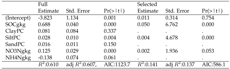
Linear regression models of STN and for STP were constructed from the six covariates and a stepwise AIC model selection procedure was applied. Tables 1 and 2 summarize the coefficient estimates and the selected covariates.

Full Selected

Estimate Std. Error Pr(>|t|) Estimate Std. Error Pr(>|t|)

(Intercept) -3.823 1.134 0.001 0.011 0.314 0.754

SOCgkg 0.688 0.040 0.000 0.050 6.762 0.000

ClayPC 0.081 0.084 0.337 . . .

SiltPC 0.028 0.010 0.004 0.004 4.678 0.000

SandPC 0.016 0.011 0.150 . . .

NO3Ngkg 0.125 0.029 0.000 0.002 1.936 0.053

NH4Ngkg -0.138 0.074 0.061 . . .

R2:0.610 adjR2:0.607, AIC:1123.7 R2:0.141 adjR2:0.137 AIC:586.1

Table 1: Summary of the coefficient estimates arising from the Full and AIC selected linear regression models of STN.

Full Selected

Estimate Std. Error Pr(>|t|) Estimate Std. Error Pr(>|t|)

(Intercept) -0.078 0.163 0.632 0.201 0.014 0.000

SOCgkg 0.047 0.006 0.000 0.014 0.002 0.000

ClayPC 0.011 0.012 0.366 -0.005 0.002 0.002

SiltPC 0.007 0.001 0.000 0.004 0.000 0.000

SandPC 0.005 0.002 0.002 . . .

NO3Ngkg -0.001 0.004 0.866 . . .

NH4Ngkg 0.026 0.011 0.013 0.001 0.001 0.023

R2:0.404 adjR2:0.399 AIC:-1548.2 R2:0.326 adjR2:0.322 AIC:-1178.9

Table 2: Summary of the coefficient estimates arising from the Full and AIC selected linear regression models of STP.

SOCgkg, SiltPC, SandPC, and NH4Ngkg with anR2_{value of 0.40, again similar to the} find-ings of Wang et al (2009). The selected model did not include the covariates for NO3Ngkg and SandPC, but all retained covariates were significant. In both cases the selected models reflect the impact of silt and soil organic carbon in increasing the soil surface area sup-porting higher absorption capacities, and thus concentrations of STN and STP, as noted by Wang et al. [41]. The AIC selected models are more parsimonious model but with weaker

R2_{and adjustedR}2_{values as would be expected.}

Note that the selected model does not necessarily include covariates that are significant and that non-significant covariates in the full model may be included in the selected model and may become significant (e.g., the ClayPC covariate for the STP regression). The key point is that the variance in STN and STP can be explained by two competing, but equally valid linear regression models. This concept is repeated locally in the subsequent GWR analyses and is a cornerstone of this paper.

3.2

Standard GWR

Linear regression models assume that the contributions to the model made by the different covariates are the same across the study area. In reality, this assumption of process spatial invariance may be violated and GWR seeks to quantify the spatial variation in data rela-tionships. In a standard GWR analysis, covariate selection is typically undertaken globally and the same regression model is constructed locally using weighted data subsets. The coefficient estimates are commonly mapped and local covariate selection (and goodness of fit evaluations) can be done by identifying local covariatet-values that indicate coefficients to be significantly different from zero (e.g., [24]).

note the relatively high variation of the IQRs of the local coefficient estimates in the GWR models compared to the global coefficient estimates.

1st Qu. Median Mean 3rd Qu. IQR Global

Intercept -4.9409 -2.8261 -3.0396 -0.8880 4.0529 -3.8229

SOCgkg 0.6137 0.6730 0.6760 0.7509 0.1372 0.6882

ClayPC -0.0162 0.0865 0.0752 0.1630 0.1792 0.0811

SiltPC 0.0012 0.0166 0.0201 0.0390 0.0378 0.0284

SandPC -0.0092 0.0068 0.0099 0.0315 0.0407 0.0156

NO3Ngkg 0.0399 0.0909 0.1282 0.1666 0.1267 0.1247

NH4Ngkg -0.2313 -0.1115 -0.1661 -0.0395 0.1918 -0.1384

Table 3: The distributions of the coefficient estimates arising from a GWR model of STN.

1st Qu. Median Mean 3rd Qu. IQR Global

Intercept -0.2119 -0.1046 -0.0683 0.0640 0.2759 -0.0781

SOCgkg 0.0371 0.0410 0.0422 0.0487 0.0116 0.0469

ClayPC -0.0130 0.0132 0.0063 0.0261 0.0391 0.0110

SiltPC 0.0059 0.0081 0.0078 0.0098 0.0039 0.0074

SandPC 0.0038 0.0050 0.0051 0.0061 0.0023 0.0049

NO3Ngkg -0.0016 0.0027 0.0031 0.0061 0.0077 -0.0007

NH4Ngkg 0.0000 0.0186 0.0180 0.0412 0.0412 0.0263

Table 4: The distributions of the coefficient estimates arising from a GWR model of STP.

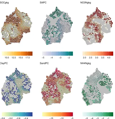
The spatial variations in the coefficient estimates arising from the two GWR models are mapped in Figures 2 and 3 and indicate the relative importance of the contribution made to each local model by each covariate at each location. They confirm that there is much greater spatial variation in the relationships associated with STN than with STP.

Thet-values in Figures 2 and 3 show where local coefficients are significant and thus where a covariate is an important predictor of STN or STP. This provides an indication of local covariate selection from the full model and is analogous to the global full models reported in Tables 1 and 2. For example, it is evident in both GWR models that SOCgkg is strongly and significantly associated with STN and STP across all locations, but the strength of this association varies spatially. Whereas significant coefficient estimates of NO3Ngkg are highly localized in each GWR model indicting strong associations in the north east and center of the study area with STN and strong associations in the north with STP. In general, significant relationships are much more localized for STN than for STP.

3.3

Hyper-local GWR

0.5 0.6 0.7 0.8 0.9 SOCgkg

−0.2 0.0 0.2 0.4 ClayPC

0.00 0.03 0.06 SiltPC

0.00 0.05 SandPC

0.0 0.2 0.4 0.6

NO3Ngkg

−0.8 −0.6 −0.4 −0.2 0.0 NH4Ngkg

Figure 2: Spatial variation in coefficient estimates from a standard GWR model of STN. Significantt-values are indicated by the black shaded points.

0.5 0.6 0.7 0.8 0.9 SOCgkg

−0.2 0.0 0.2 0.4 ClayPC

0.00 0.03 0.06 SiltPC

0.00 0.05 SandPC

0.0 0.2 0.4 0.6

NO3Ngkg

−0.8 −0.6 −0.4 −0.2 0.0 NH4Ngkg

Figure 3: Spatial variation in coefficient estimates from a standard GWR model of STP. Significantt-values are indicated by the black shaded points.

For each of the 689 data points, the hyper-local GWR identified the components of the best fitting model for each of the 63 bandwidths (from 200 m to 3700 m in intervals of 50 m) and returned the AIC score for the model. Thus it was possible to determine the best fitting model, with the lowest AIC score at each location.

3.3.1 Local bandwidth selection

Bandwidth 500 1000 1500

STN

Bandwidth 2000 2500 3000 3500

STP

Figure 4: Spatial variation in local bandwidth size (in metres) of the hyper-local GWR mod-els of STN and STP.

from the southeast to the northwest. This suggests that local regressions in this area are in-formed by data subsets of a similar size to that found with standard GWR (with its constant bandwidth of 1026 m). Elsewhere, the bandwidths are much smaller (200-1000 m), so that local regressions in these areas are informed by much smaller data subsets. The distribu-tion of bandwidths in the hyper-local GWR model is on the whole indicative of increased localized spatial heterogeneity in data relationships, which is more than that suggested by the standard GWR analyses above.

Conversely, the STP bandwidths range from 1500-3700 m and are much larger almost everywhere than the constant bandwidth for standard GWR at 1629 m. Thus, most of the local regressions in a hyper-local GWR are informed by much larger data subsets than a standard GWR. Only to the center of the study area are bandwidths from hyper-local GWR of similar size to a standard GWR. The larger bandwidths indicate reduced spatial heterogeneity to that found with standard GWR, and suggests spatial homogeneity in the relationships (i.e., tending to the global regression).

3.4

Local covariate selection and distribution of coefficient t-values

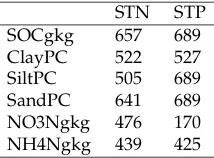
these are now selected in 522, 641, and 439 out of 689 hyper-local models, respectively). STP model selection for the global regression (Table 2) excluded SandPC and NO3Ngkg, while these are now selected in 689 and 170 out of 689 local models, respectively). Addi-tionally, three covariates were always selected regression (SOCgkg, SiltPC, and SandPC), whereas for STN none were. This suggests that there are potentially interesting local inter-actions between covariates which are missed in standard GWR in which all six covariates are included in the model for all 689 local regressions.

STN STP

SOCgkg 657 689

ClayPC 522 527

SiltPC 505 689

SandPC 641 689

NO3Ngkg 476 170

NH4Ngkg 439 425

Table 5: Number of sample locations where different covariates were selected in hyper-local GWR.

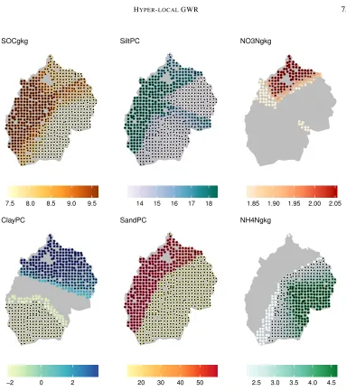
Figures 5 and 6 show the spatial variation in the selection of covariates and their coef-ficient estimates in the hyper-local GWR models and where the coefcoef-ficient estimates were found to be locally significant via theirt-values. The coefficient estimates arising from the hyper-local GWR models are summarized in Tables 6 and 7. Note that the legends in Fig-ures 5 and 6 display data values within the inter-quartile ranges of the hyper-local GWR coefficient estimates. Extreme values were set to the 25th or 75th quartile value, to provide a meaningful shading. Of interest is where the hyper-local GWR coefficients were found to be significant via theirt-values and how these compare to the maps oft-values in Figures 2 and 3 for standard GWR. Some large local differences are evident, especially for STN.

For example, in the STN models (comparing Figures 2 and 5), SandPC is a significant covariate at most locations in the hyper-local GWR model. In the standard GWR model (Figure 2 it is only significant in two sub-regions to the north and center of the study area. Whilst, NH4Ngkg in the standard GWR model of STN is significant in the north-west of the study area, but has a much wider significance in the hyper-local GWR model. These results indicate that when the bandwidth and covariate selection are more localized under the hyper-local GWR, then significant non-stationary relationships result, that are not apparent with standard GWR. Similar interpretations apply to STN relationships with SiltPC, NO3Ngkg, and ClayPC while it appears that STN’s relationship to SOCgkg is con-sistent across both GWR forms. Note also that hyper-local GWR tends to provide spatially disjoint areas of covariate selection and coefficient significance, reflecting highly localized processes. For the STP process, comparing Figures 3 and 6, there are very similar patterns for significant coefficients from the hyper-local GWR and from the standard GWR for all six covariates, although NO3Ngkg, SandPC, ClayPC, and NH4Ngkg show enlarged localized areas of significance under the hyper-local model. Note that NO3Ngkg is only selected in 170 sample locations in hyper-local GWR (see Table 5) and these are in the north, precisely where the standard GWR shows the NO3Ngkg relationships as significant.

However, where localized spatial heterogeneity is present in data relationships, as with STN, the hyper-local GWR provides a more spatial nuanced indication of the localization than a standard GWR analysis.

10.0 12.5 15.0 17.5

SOCgkg

−3.6 −3.2 −2.8 −2.4

ClayPC

−5 −4 −3 −2

SiltPC

−15 −10 −5

SandPC

2.0 2.5 3.0 3.5 4.0

NO3Ngkg

−5 −4 −3 −2 −1

NH4Ngkg

Figure 5: The spatial distribution of the selected covariates included in each hyper-local GWR model of STN. Significantt-values are indicated by the black shaded points.

3.5

Comparisons of global and local model fit

increas-7.5 8.0 8.5 9.0 9.5

SOCgkg

−2 0 2

ClayPC

14 15 16 17 18

SiltPC

20 30 40 50

SandPC

1.85 1.90 1.95 2.00 2.05

NO3Ngkg

2.5 3.0 3.5 4.0 4.5

NH4Ngkg

Figure 6: The spatial distribution of the selected covariates included in each hyper-local GWR model of STP. Significantt-values are indicated by the black shaded points.

ing spatial nuance, from linear regression (full model), to standard GWR and to hyper-local GWR (R2 _{of 0.61, 0.68 and 0.94, respectively). Rather surprisingly, there is little} improve-ment in model fit from the linear regression to standard GWR. The strong predictive per-formance of hyper-local GWR can be attributed to the local tightening of bandwidths and variable selection. For STP, the model fits do not improve in the same way. There is a moderate increase from linear regression (full model) to standard GWR but then a small decrease to the hyper-local GWR (R2_{of 0.40, 0.47, and 0.45 respectively). The decrease in}

1st Qu. Median Mean 3rd Qu.

SOCgkg 8.3827 13.7124 15.1081 19.1944

ClayPC -3.6305 -2.7275 -3.8169 -2.0444

SiltPC -5.1766 -3.2462 -4.0274 -1.4613

SandPC -19.4445 -8.8947 -14.0557 -4.8087

NO3Ngkg 1.8363 3.1133 2.7784 4.3087

NH4Ngkg -5.7028 -3.2104 -2.6720 -0.1863

Table 6: The distributions of the coefficient estimates arising from the hyper-local GWR model of STN.

1st Qu. Median Mean 3rd Qu.

SOCgkg 7.4957 8.4218 8.5008 9.6309

ClayPC -2.3965 1.8810 1.0432 3.9876

SiltPC 13.3632 15.3115 18.3168 18.4171

SandPC 12.1923 13.4488 31.7100 59.7112

NO3Ngkg 1.8337 1.9602 1.7673 2.0503

NH4Ngkg 2.2802 3.4096 3.5812 4.6855

Table 7: The distributions of the coefficient estimates arising from the hyper-local GWR model of STN.

standard GWR, as the bandwidths for hyper-local GWR tend to be larger and the process tends towards the global fit.

Care must be taken in the interpretation of model fit results, as any form of localized regression will tend to provide an improved prediction accuracy, the more complex it gets (hence the strong performance of local GWR for STN). Furthermore, although hyper-local GWR is shown to improve fit for the STN process, this has little predictive value, as hyper-local GWR cannot be used as an of-sample predictor. This is because the out-of-sample prediction does not have its own local bandwidth, whereas for standard GWR, the global bandwidth can be used [23]. Thus, hyper-local GWR is solely for guiding spatial exploration and inference only, as demonstrated in this study.

It is important to investigate local model fit characteristics so that the outputs in Figures 2 to 6 can be placed in better context and geographically contrasted. Figure 8 compares the localR2 _{values for standard GWR and hyper-local GWR models for STN and STP and} indicates that hyper-local GWR provides a better fit in 503/689 and 5/689 locations for STN and STP, respectively. Thus, for the STN process, the local regressions of standard GWR could be considered sub-optimal in 73% of the locations, whilst for the STP process, the local regressions of standard GWR are, in general, reasonable. The magnitude of the differences are much greater for STN than for STP. If Figure 8 is compared with Figure 4, the areas where a hyper-local approach provides a better model fit for STN directly corre-spond to those where a much smaller local bandwidth was selected. This behavior is not so apparent for the STP process.

−3 −2 −1 0

−7.5 −5.0 −2.5 0.0 2.5

Observed

Fitted

STN Linear Regression r 2 =0.61 −4 −3 −2 −1 0

−7.5 −5.0 −2.5 0.0 2.5

Observed

Fitted

STN GWR r 2_=0.679

−9 −6 −3 0

−7.5 −5.0 −2.5 0.0 2.5

Observed

Fitted

STN Hyper Local GWR r 2 =0.935 0.5 0.6 0.7 0.5 1.0 Observed Fitted

STP Linear Regression r

2 =0.404 0.4 0.5 0.6 0.7 0.8 0.5 1.0 Observed Fitted

STP GWR r

2_=0.467

0.4 0.5 0.6 0.7 0.5 1.0 Observed Fitted

STP Hyper Local GWR r

2 =0.454

Difference 0.1 0.2 0.3 Model GWR Hyper−Local

STN

Difference 0.005 0.010 0.020 Model GWR Hyper−Local STP

Figure 8: Maps of the difference in localR2_{values under standard GWR and hyper-local} GWR models. Locations in red indicate where a hyper-local GWR model resulted in a better fitting model and (black for GWR) and the size of the plot characters indicate the magnitude of the difference.

well-informed by the six covariates. For STP, hyper-local GWR suggests more moderately spatially-varying relationships but where local model fits are similar (slightly weaker) to that found for standard GWR. Thus, the application of hyper-local GWR provides little value to an extended use of nearby data points with often fewer covariates for its local regressions. The STP process, is in general, not well-informed by the six covariates.

4

Discussion

GWR is an inherently exploratory approach for examining and investigating process non-stationarity in data relationships. The hyper-local GWR extends these investigations fur-ther. Whereas a standard GWR employs a one-size-fits-all bandwidth and a one-size-fits-all local regression model, the hyper-local GWR approach evaluates different kernel band-widths and models at each location. It provides an alternative and complementary in-terpretation of localized regression by locally selecting the most parsimonious model (by local sample and covariate size), for which spatially distributed coefficient estimates and

The investigations show that where the non-stationarity of relationships tend towards the global, as with STP, the results are similar to a standard GWR (compare Figures 3 and 6). However, where localized spatial heterogeneity and spatial non-stationarityarepresent, as with STN, the hyper-local GWR provides a more spatially nuanced indication of the localization than a standard GWR analysis (compare Figures 2 and 5). Thus the hyper-local GWR results can be used to guide the direction of the next analytical steps. Further anal-ysis of the STN could consider adopting a more sophisticated spatially-varying coefficient model (e.g., [18]), including models that accounts for non-linearity (e.g., [2]). Further analy-sis of STP could consider a spatially-autocorrelated regression given that its GWR analyses were not entirely promising (e.g., [21]).

Determining local bandwidth size and local covariate selection is also in the same spirit as (but with entirely different objectives to) the GWR models of Paez et al. [34, 35], Wheeler [42], and Yoneoka et al. [43]. These are analogous to developments in local (attribute-space) regression [29, 40] from which GWR originates [5, 31], but the GWR models of Paez only do local bandwidths (not local covariate selection) and the GWR models of Wheeler and Yoneoka only do local covariate selection (not local bandwidths). The exploratory and en-hanced spatial nuance of hyper-local GWR reflects recent developments within the broad family of GWR methods that has promoted wider consideration of scale and distance. These include hierarchical GWR models [25], consideration of distance metrics [10, 30], and flexible bandwidth GWR models [17, 26] that select different bandwidths for each de-pendent/independent data relationship, rather than for each location as here. These multi-scale GWR models are closely aligned to the spatially-varying coefficient models of Gelfand et al. [18] and Murakami et al. [32].

There is a computational cost to hyper-local GWR approaches which evaluate a model for each bandwidth at each location, rather than a standard GWR, which just evaluates a single bandwidth and a single model. It terms of computing time, a standard GWR using the GWmodel package v2.0-5 [19] in R took 2.96 seconds to run on this data. The hyper-local approach took longer—20.7 minutes—because of the number of calculations but also because the algorithm has been transparently (rather than efficiently) coded. The data and code used in this analysis have been made available (see the acknowledgments section).

dis-tance, as used here, or fixed by sample size), and the choice of distance metric, all of which effect perspectives of coefficient non-stationarity. It would be interesting to examine the de-gree of difference between the STN and STP standard and hyper-local GWR models under such different parameterization choices. Gollini et al. [19] provides overviews of these con-siderations. Fourth, another area of future work is to examine the potential for overfitting with hyper-local methods. One way to test whether hyper-local GWR describes the study data significantly better than standard GWR would be to adapt theF-test procedure given in Leung et al. [27]. Here, instead of assessing standard GWR against the global linear regression, hyper-local GWR is assessed against standard GWR, where the null hypothesis is no significant difference between models. A fifth and more salient consideration for the research described in this paper is the use of AIC scores to select both local bandwidths and local regression models. AIC [1, 25] seeks to optimize model parsimony by trading off prediction accuracy and complexity. Other measures of fit could be applied including some kind of cross-validation measure of residual errors. There have been a number of arguments made in the context of information theory about the choice of model selection method and their associated measures of fit, and Li and Lam [28] review variable selec-tion methods in GWR frameworks. They compared Step-AIC in GWR, GWR-Lasso, and GWR-Ridge models, noting that they are a function of zero-power, one-power, and two-power, respectively, of the explanatory variables in the models. This essentially frames the relationships between model selection within the elastic net. In terms of information cri-teria, alternatives to AIC exist such as Bayesian Information Criterion (BIC) and Deviance Information Criterion (DIC) [39]. Future work will investigate these and CV approaches as they would be expected to result in different local model selection. The key in determining which model selection method to use is to understand the logics of each approach and how they relate to the study objectives and even the underlying objectives of data collection. For example, AIC and BIC provide different approaches for model comparison [7]. BIC seeks to determine the “true” model and, if any particular candidate model represents the genuine data-generating mechanism, BIC will select such a model. It is said to be asymptotically consistent because it seeks to select the true model. By contrast AIC seeks to pragmatically select a model by trading-off explanations of the data with prediction strength. Despite these theoretical differences, Spiegelhalter et al. [38] note that “it is perhaps therefore rather surprising how often these two criteria produce similar rankings of candidate models” (p. 486) with the only real differences found in the size of the penalty scores [14]. Future work for both hyper-local and standard GWR will investigate the use of different model selection criteria, the logics associated with the local models being constructed and the underlying process spatial heterogeneity.

5

Conclusions

study). Standard GWR applies the same regression model at each location and uniformly sets the same kernel bandwidth everywhere. The hyper-local GWR approach evaluates different kernel bandwidths at each location and selects the most parsimonious local re-gression model. Where spatial non-stationarity exists, the hyper-local GWR provides a more spatially nuanced indication of the localization than a standard GWR analysis and can be used to suggest the direction of further analyses and investigations. Undertaking a hyper-local GWR alongside a standard GWR allows coefficient estimates, t-values and bandwidths to be compared for differences and similarities. Specifically, a dual GWR ap-proach that examines the spatial distribution of local covariate selection and the local band-width size supports a deeper understanding of the local and scale-related characteristics of the spatial process under investigation.

Acknowledgments

This work was supported by National Natural Science Foundation of China (NSFC) and the Natural Environment Research Council (NERC) Newton Fund through the China-UK collaborative research on critical zone science (No. 41571130083 and NE/N007433/1), the NSFC (No.41530854) and UK Biotechnology and Biological Sciences Research Council grant (BBSRC BB/J004308/1). All of the analyses and mapping were undertaken in R 3.4.3 the open source statistical software. The GWR analyses used the GWmodel package, v2.0-1 [v2.0-19]. The data and code used to generate the analysis and all of the figures and tables can accessed from https://github.com/lexcomber/hyperlocalGWR. AC conceived, and led the design and implementation of the analysis; YW collected and processed the data used in the analysis; PH guided the analysis. All authors contributed to interpreting the results, refining the analysis, and the writing of the manuscript.

References

[1] AKAIKE, H. Information theory and an extension of the maximum likelihood princi-ple. InProceedings of the 2nd Symposium on Information Theory, BN Petrov, F Csaki (eds.),

(1973), Akademiai Kiado, Budapest, pp. 267–281.

[2] BÁRCENA, M., MENÉNDEZ, P., PALACIOS, M.,ANDTUSELL, F. Alleviating the effect of collinearity in geographically weighted regression. Journal of Geographical Systems 16, 4 (2014), 441–466. doi:10.1007/s10109-014-0199-6.

[3] BASILE, R., DURBÁN, M., MÍNGUEZ, R., MONTERO, J. M., AND MUR, J. Modeling regional economic dynamics: Spatial dependence, spatial heterogeneity and nonlinearities. Journal of Economic Dynamics and Control 48 (2014), 229–245. doi:10.1016/j.jedc.2014.06.011.

[5] BRUNSDON, C., FOTHERINGHAM, A. S., AND CHARLTON, M. E. Geographically weighted regression: a method for exploring spatial nonstationarity.Geographical anal-ysis 28, 4 (1996), 281–298. doi:10.1111/j.1538-4632.1996.tb00936.x.

[6] BRUNSDON, C., FOTHERINGHAM, S.,ANDCHARLTON, M. Geographically weighted

discriminant analysis. Geographical Analysis 39, 4 (2007), 376–396. doi:10.1111/j.1538-4632.2007.00709.x.

[7] BURNHAM, K. P., AND ANDERSON, D. R. Multimodel inference: understanding AIC and BIC in model selection. Sociological methods & research 33, 2 (2004), 261–304. doi:10.1177/0049124104268644.

[8] CHILÈS, J.,ANDDELFINER, P. Geostatistics: Modeling spatial uncertainty.John Wiley & Sons, New York., 1999.

[9] COMBER, A., BRUNSDON, C., CHARLTON, M., AND HARRIS, P. Geographically weighted correspondence matrices for local error reporting and change analyses: mapping the spatial distribution of errors and change. Remote Sensing Letters 8, 3 (2017), 234–243. doi:10.1080/2150704X.2016.1258126.

[10] COMBER, A., CHI, K., QUANGHUY, M., NGUYEN, Q., LU, B., HUU PHE, H., AND

HARRIS, P. Distance metric choice can both reduce and induce collinearity in geo-graphically weighted regression.Environment and Planning B: Urban Analytics and City Science(2018). doi:10.1177/2399808318784017.

[11] COMBER, A., LI, T., LÜ, Y., FU, B.,ANDHARRIS, P. Geographically weighted struc-tural equation models: spatial variation in the drivers of environmental restoration effectiveness. InSocietal Geo-Innovation. 20th AGILE Conference Proceedings, 2017.

[12] COMBER, A. J. Geographically weighted methods for estimating local surfaces of overall, user and producer accuracies. Remote Sensing Letters 4, 4 (2013), 373–380. doi:10.1080/2150704X.2012.736694.

[13] DA SILVA, A. R., AND FOTHERINGHAM, A. S. The multiple testing issue in geographically weighted regression. Geographical Analysis 48, 3 (2016), 233–247. doi:10.1111/gean.12084.

[14] DZIAK, J. J., COFFMAN, D. L., LANZA, S. T.,ANDLI, R. Sensitivity and specificity of

information criteria.PeerJ PrePrints(2017). doi:10.7287/peerj.preprints.1103v3.

[15] FOODY, G. Local characterization of thematic classification accuracy through spatially constrained confusion matrices. International Journal of Remote Sensing 26, 6 (2005), 1217–1228. doi:10.1080/01431160512331326521.

[16] FOTHERINGHAM, A. S., BRUNSDON, C.,ANDCHARLTON, M.Geographically Weighted Regression: the Analysis of Spatially Varying Relationships. Wiley, Chichester, 2002.

[18] GELFAND, A. E., KIM, H.-J., SIRMANS, C.,ANDBANERJEE, S. Spatial modeling with spatially varying coefficient processes.Journal of the American Statistical Association 98, 462 (2003), 387–396. doi:10.1198/016214503000170.

[19] GOLLINI, I., LU, B., CHARLTON, M., BRUNSDON, C.,ANDHARRIS, P. Gwmodel: an

R package for exploring spatial heterogeneity using geographically weighted models.

Journal of Statistical Software 63, 17 (2015), 1–50. doi:10.18637/jss.v063.i17.

[20] HARRIS, P., BRUNSDON, C.,ANDCHARLTON, M. Geographically weighted principal components analysis. International Journal of Geographical Information Science 25, 10 (2011), 1717–1736. doi:10.1080/13658816.2011.554838.

[21] HARRIS, P., BRUNSDON, C., LU, B., NAKAYA, T., AND CHARLTON, M. Introduc-ing bootstrap methods to investigate coefficient non-stationarity in spatial regression models.Spatial Statistics 21(2017), 241–261. doi:10.1016/j.spasta.2017.07.006.

[22] HARRIS, P., CHARLTON, M., ANDFOTHERINGHAM, A. S. Moving window kriging with geographically weighted variograms. Stochastic Environmental Research and Risk Assessment 24, 8 (2010), 1193–1209.

[23] HARRIS, P., FOTHERINGHAM, A., CRESPO, R.,ANDCHARLTON, M. The use of geo-graphically weighted regression for spatial prediction: an evaluation of models using simulated data sets.Mathematical Geosciences 42, 6 (2010), 657–680. doi:10.1007/s11004-010-9284-7.

[24] HARRISP, FOTHERINGHAMAS, J. S. Robust geographically weighted regression: a technique for quantifying spatial relationships between freshwater acidification criti-cal loads and catchment attributes. Annals of the Association of American Geographers. 100, 2 (2010), 286–306. doi:10.1080/00045600903550378.

[25] HURVICH, C. M., SIMONOFF, J. S.,ANDTSAI, C.-L. Smoothing parameter selection in nonparametric regression using an improved akaike information criterion. Journal of the Royal Statistical Society: Series B (Statistical Methodology) 60, 2 (1998), 271–293. doi:10.1111/1467-9868.00125.

[26] LEONG, Y.-Y.,ANDYUE, J. C. A modification to geographically weighted regression.

International journal of health geographics 16, 1 (2017), 11. doi:10.1186/s12942-017-0085-9.

[27] LEUNG, Y., MEI, C.-L.,ANDZHANG, W.-X. Statistical tests for spatial nonstationarity

based on the geographically weighted regression model. Environment and Planning A 32, 1 (2000), 9–32. doi:10.1068/a3162.

[28] LI, K.,ANDLAM, N. S. Geographically weighted elastic net: A variable-selection and modeling method under the spatially nonstationary condition. Annals of the American Association of Geographers(2018), 1–19. doi:10.1080/24694452.2018.1425129.

[29] LOADER, C. Smoothing: local regression techniques. InHandbook of Computational Statistics. Springer, 2012, pp. 571–596. doi:10.1007/978-3-642-21551-3\_20.

[31] MCMILLEN, D. P., AND MCDONALD, J. F. A nonparametric analysis of employ-ment density in a polycentric city. Journal of Regional Science 37, 4 (1997), 591–612. doi:10.1111/0022-4146.00071.

[32] MURAKAMI, D., YOSHIDA, T., SEYA, H., GRIFFITH, D. A., AND YAMAGATA, Y. A Moran coefficient-based mixed effects approach to investigate spatially varying rela-tionships.Spatial Statistics 19(2017), 68–89. doi:10.1016/j.spasta.2016.12.001.

[33] OPENSHAW, S. Developing GIS-relevant zone-based spatial analysis methods.Spatial analysis: modelling in a GIS environment(1996), 55–73.

[34] PÁEZ, A., UCHIDA, T.,ANDMIYAMOTO, K. A general framework for estimation and inference of geographically weighted regression models: 1. location-specific kernel bandwidths and a test for locational heterogeneity. Environment and Planning A 34, 4 (2002), 733–754. doi:10.1068/a34110.

[35] PÁEZ, A., UCHIDA, T., AND MIYAMOTO, K. A general framework for estimation and inference of geographically weighted regression models: 2. spatial association and model specification tests. Environment and Planning A 34, 5 (2002), 883–904. doi:10.1068/a34133.

[36] RIPLEY, B., VENABLES, B., BATES, D. M., HORNIK, K., GEBHARDT, A., FIRTH, D.,

ANDRIPLEY, M. B. Package ‘mass’.Cran R(2013).

[37] SHEN, S.-L., MEI, C.-L., AND ZHANG, Y.-J. Spatially varying coefficient models: testing for spatial heteroscedasticity and reweighting estimation of the coefficients.

Environment and Planning A 43, 7 (2011), 1723–1745. doi:10.1068/a43201.

[38] SPIEGELHALTER, D. J., BEST, N. G., CARLIN, B. P., AND LINDE, A. The deviance information criterion: 12 years on. Journal of the Royal Statistical Society: Series B (Sta-tistical Methodology) 76, 3 (2014), 485–493. doi:10.1111/rssb.12062.

[39] SPIEGELHALTER, D. J., BEST, N. G., CARLIN, B. P., AND VAN DER LINDE, A. Bayesian measures of model complexity and fit. Journal of the Royal Statistical Society: Series B (Statistical Methodology) 64, 4 (2002), 583–639. doi:10.1111/1467-9868.00353.

[40] VIDAURRE, D., BIELZA, C., AND LARRAÑAGA, P. Lazy lasso for local regression.

Computational Statistics 27, 3 (2012), 531–550. doi:10.1007/s00180-011-0274-0.

[41] WANG, Y., ZHANG, X., AND HUANG, C. Spatial variability of soil

to-tal nitrogen and soil toto-tal phosphorus under different land uses in a small watershed on the Loess Plateau, China. Geoderma 150, 1-2 (2009), 141–149. doi:10.1016/j.geoderma.2009.01.021.

[42] WHEELER, D. C. Simultaneous coefficient penalization and model selection in geo-graphically weighted regression: the geogeo-graphically weighted lasso. Environment and planning A 41, 3 (2009), 722–742. doi:10.1068/a40256.