Polymers and biopolymers at interfaces

(1)

This is a repository copy of Polymers and biopolymers at interfaces. White Rose Research Online URL for this paper:

http://eprints.whiterose.ac.uk/127050/ Version: Accepted Version

Article:

Hall, A.R. and Geoghegan, M. (2018) Polymers and biopolymers at interfaces. Reports on Progress in Physics, 81 (3). 036601. ISSN 0034-4885

https://doi.org/10.1088/1361-6633/aa9e9c

[email protected] https://eprints.whiterose.ac.uk/ Reuse

Items deposited in White Rose Research Online are protected by copyright, with all rights reserved unless indicated otherwise. They may be downloaded and/or printed for private study, or other acts as permitted by national copyright laws. The publisher or other rights holders may allow further reproduction and re-use of the full text version. This is indicated by the licence information on the White Rose Research Online record for the item.

Takedown

If you consider content in White Rose Research Online to be in breach of UK law, please notify us by

(2)

Polymers and biopolymers at interfaces

A R Hall1,2 _{and M Geoghegan}1

1 Department of Physics and Astronomy, University of Sheffield, Hounsfield Road, Sheffield S3 7RH, UK

2 Biomedical Diagnostics Institute, Dublin City University, Glasnevin, Dublin 9, Ireland

Abstract.

This review updates recent progress in the understanding of the behaviour of polymers at surfaces and interfaces, highlighting examples in the areas of wetting, dewetting, crystallization, and “smart” materials. Recent developments in analysis tools have yielded a large increase in the study of biological systems, and some of these will also be discussed, focussing on areas where surfaces are important. These areas include molecular binding events and protein adsorption as well as the mapping of the surfaces of cells. Important techniques commonly used for the analysis of surfaces and interfaces are discussed separately to aid the understanding of their application.

1. Introduction

(3)

List of abbreviations

AFM atomic-force microscopy DLVO Derjaguin, Landau, Verwey,

and Overbeek

F8 poly(9,9-dioctylfluorene) F8BT

poly(9,9-dioctylfluorene-alt-benzothiadiazole)

FCS fluorescence correlation

spectroscopy

FFM friction force microscopy

FJC freely-jointed chain FPE fish protein extract

FReS forward recoil spectrometry HSA human serum albumin

LCST lower critical solution

tem-perature

LED light-emitting diode

NRA nuclear reaction analysis PDMAc poly(N,N

-dimethylacrylamide)

PDMS polydimethylsiloxane PEDOT poly(3,4-ethylene

dioxythiophene)

PEG poly(ethylene glycol) PET poly(ethylene terepthalate)

PFB

poly(9,9-dioctylfluorene-alt-bis-N,N′ -(4-

butylphenyl)-bis-N,N′ -phenyl-1,4-phenylenediamine)

PLLA poly(l-lactic acid)

PMAA poly(methacrylic acid) PNIPAm poly(N-isopropyl

acry-lamide)

PSS poly(styrene sulfonate) PVME polyvinylmethylether

PαMS poly(α-methylstyrene) P3HT poly(3-hexylthiophene)

QCM-D quartz crystal microbalance

with dissipation

RBS Rutherford backscattering

SBA soybean agglutinin SEM scanning electron

mi-croscopy

SFM scanning force microscopy SIMS secondary-ion mass

spec-trometry

SMFS single molecule force

spec-troscopy

SNOM scanning near-field optical

microscopy

STM scanning tunnelling

mi-croscopy

TCPS tissue culture polystyrene

TIPS-pentacene 6,13-bis(triisopropylsilyl ethynyl) pentacene

TnPSM modified porcine

submaxil-lary mucin

UHV ultra-high vacuum UV ultraviolet

UPS ultraviolet photoelectron

spectroscopy

WLC worm-like chain

XPS X-ray photoelectron

(4)

tend to also be compatible with the solvent. Therefore the following interactions need to be considered in order to describe the energetics of adsorption: polymer-solvent, solvent-solvent, polymer-polymer, polymer-surface, and solvent-surface. The free energy of a polymer in solution is typically a few kBT. It is not possible to be too precise about

this. After all, the energy of a gaseous atom is3kBT /2, but make it a diatomic molecule

and that energy can rise to 7kBT /2, if rotational and vibrational modes are excited.

A polymer is solution contains many modes that may or may not be excited, so it is reasonable to note that individual interactions are of the order ofkBT. This means that

a polymer with Ns monomers in contact with a surface has an adsorption energy of the

order of NskBT. Fundamentally, this is why polymers stick to surfaces. They stick to

surfaces because out of the many competing interactions, the adsorption of a polymer at a surface is so much stronger than the adsorption of solvent molecules to that surface.

(a)

(b)

(c)

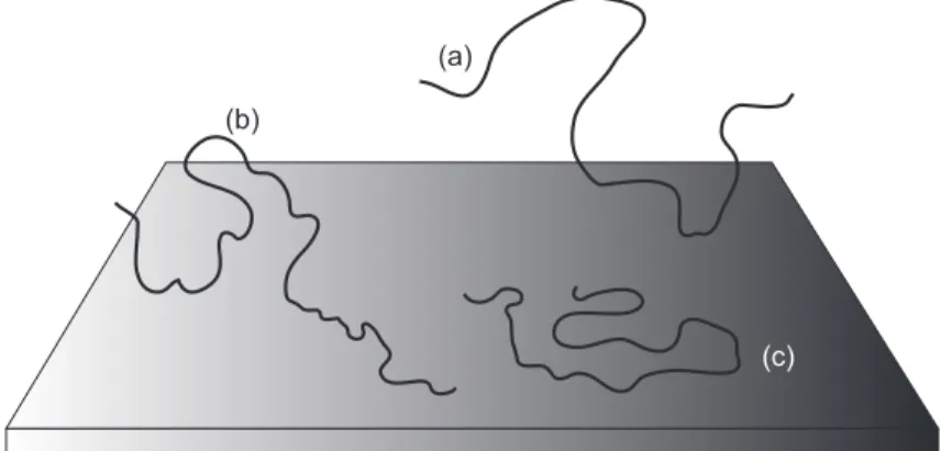
Figure 1. A polymer may have only one anchor point (a) on the surface, with the

rest of the molecule spreading out into the solution. Other polymers may make more contact, with trains of many monomers in contact with the surface, loops into the solution, and solvated ends known astails (b). The “pancake” conformation refers to polymers that are almost wholly attached to the substrate (c)

(5)

microscopy (AFM) and other techniques such as optical tweezers that were capable of manipulating single macromolecules.

The review by Krausch [2] took as a starting point the idea that differences in surface energy between different components of a polymer blend thin film or a block copolymer-induced structure gave surfaces their individual properties. The first experiments in this area were speculative and of value largely for the interesting results they presented. Reich and Cohen [5] presented optical microscopy results that showed phase separation in films of blends of polystyrene and polyvinylmethylether (PVME). It was some years later that a different team showed that the PVME in this blend was found at the surface in greater concentrations than in the bulk of the film [6], solely due to the differences in surface energy between the two components. The increasing access of good technology to different research groups ensured that such important results could be made. Here X-ray photoelectron spectroscopy (XPS) was used to identify PVME at the surface, and the simpler pendant drop experiment to contrast the surface energies of the two components. Theoretically, it was realized that polymers at surfaces could be treated adequately by mean-field theory. Here the lattice model of polymer physics, pioneered by Paul Flory and others over 60 years ago [7, 8, 9], was married to the mean-field theory of wetting by John Cahn [10] to provide a theoretical foundation for the study of surface structure in polymer films [11]. Experimentally, the work of Richard Jones and Ed Kramer at Cornell University provided an application of the new theory to thin films of mixtures of polystyrene and its deuterated counterpart [12]. This work continued at pace, and some of the developments are considered later in this review. It has to be conceded nevertheless, that the structure of polymer films, as applied to homopolymer mixtures, is a subject considered “done” by many. Of course there are always new and interesting results, such as the study of polymer film formation in situ during

spin-coating [13, 14, 15, 16, 17, 18], which is a popular method of producing uniform films by rotating a drop of solution on a substrate at a few thousand rpm.

The study of single molecules on surfaces or at interfaces can be split into two categories. Some experiments manipulate individual molecules and others describe dilute mixtures whereby the behaviour of single molecules is observed, but only as an ensemble average [19]; many molecules are measured, but it is only by virtue of these molecules being very dilute that the study can be considered a single molecule experiment. The advantage of this latter scenario is that the experiments identify general behaviour, whereas in the former case there is the risk that an experiment may be performed on outlying samples. Thus reliable data for individual molecules

(6)

molecules level. FCS in particular has the ready capability of determining the number of molecules per unit volume, which is particularly useful given that what might be dilute (at the single molecule level) in the medium to which it is introduced, may not be so dilute at the surface. Experiments capable of studying individual molecules include optical tweezers, AFM, and high-resolution fluorescence microscopy experiments.

The study of ensemble behaviour of single molecules at surfaces is certainly a minority interest. Its headline experiments have involved the diffusion of polymers at surfaces using FCS [19, 20, 21, 22]. Molecular tracking has had considerable success in different areas, and particularly in cell biology [19]. High-resolution fluorescence microscopy has a role to play, and single polymer imaging has been demonstrated [23], but with further developments underway, such as stochastic optical reconstruction microscopy [24], again inspired by the needs of cell biology research, thein situ imaging

of the behaviour of single molecules is one that promises to yield important results in the coming years. Of course, AFM-based techniques do provide single molecule resolution, either by AFM itself [25] or through scanning tunnelling microscopy (STM) [26]. STM has long been known for its atomic resolution, but with its restriction on substrates often inconvenient, it is worth noting the progress of AFM in this respect [27]. The resolution of torsional mode AFM [25] is better than 0.4 nm, so there is good reason to expect routine atomic resolution in polymers in the future. Nevertheless, scanning probe techniques (AFM and STM) are techniques used to study static phenomena and their insight into the behaviour of polymers at interfaces is less likely to reveal new physics than dynamic techniques such as those that are fluorescence-based, despite the better resolution of the scanning probe microscopy experiments. (Scanning probe microscopy will have certainly a large impact in solving different kinetic problems, for example, self-assembly problems such as crystallization, where video rate scanning probe techniques have already been shown to be useful [28]. In fact more recent developments have imaged biological action at work, with video imaging of the myosin molecular motor [29].) The high resolution of electron microscopy would be expected to make some impact in the study of single molecules at surfaces, but sample preparation and contrast limitations have minimized its effectiveness, although cryo-techniques can be effective at considering surface-bound molecules [30]. Single molecule microscopy studies are considered in reviews elsewhere [19, 31].

Molecular force probe techniques are a class of AFM in which a molecule, attached to an AFM tip, is brought to, and pulled away from a surface. In some cases the polymer rests on the surface, and the AFM probe is used to study the forces involved in its removal from the surface. This is known as single molecule force spectroscopy (SMFS) and these experiments provide significant insight into the structural properties of the individual molecules at surfaces. An important contribution of experiments of this type has been to the understanding of the folding behaviour for proteins [32, 33] and the study of microbial surfaces [34]. We consider the impact of these techniques in some detail in this review.

(7)

[35]. Polymer electronic devices are prepared in film form; displays consist of a series of films, containing layers of pixels, electrodes, transistors, or transparent protecting films. The polymeric components have to be prepared in a way so as to be compatible with the layer with which it is in contact. At one level this is a matter of macroscopic physics. There is no point in putting a low work function polymer in contact with an anode because low work function polymers are not generally very good for hole transport [36, 37, 38]. However, even in pure semiconductor physics, interfaces play an important role in devices [37]. The interfaces between dissimilar materials cause traps, and equalization of Fermi levels cause internal charge flow and band-bending, which, in

turn, affects device performance. However, from the perspective of this review, the way in which the morphological evolution of structure affects the performance of devices is of some interest. Certainly, charge transport is affected by the morphology of the film. Isolated domains are effective traps for different components, so continuous structures are to be preferred. However, in some cases, such as photovoltaic devices, interfaces are required because it is atheterojunctions where the excited state (exciton) caused by the

absorption of a photon is converted into charge and thus, by the application of a bias voltage, a current is generated.

1.1. Biopolymers

An understanding of the behaviour of biopolymers at interfaces is often considered important for negative reasons. Biopolymers foul interfaces, and the unfeasibly large

technological subdomain of PEGylation is designed with the prevention of proteins reaching interfaces. PEGylation — the attachment of poly(ethylene glycol) (PEG) to surfaces or functional molecules such as drugs — is a standard technique to create biocompatibility. The Oxford English Dictionary defines compatible as meaning

(8)

The prokaryotic cell wall is a complex environment consisting of many proteins, biosurfactants, and polysaccharides. Their adhesion is controlled by adhesin molecules,

and the process of adhesion involves the secretion of these molecules to test the viability of a surface. Adhesins are part of a broader class of molecule known to biologists

as virulence factors, but for our purposes we can take them to be either proteins or

polysaccharides. If these molecules are compatible with a surface, the cell will adhere to that surface, and a biofilm may form: the surface is not biocompatible. It is common practice for researchers to consider the cell as an inert colloidal particle and its adsorption to be controlled by electrostatic and van der Waals forces. The application of theory based on these ideas — Derjaguin, Landau, Verwey, and Overbeek (DLVO) theory [41] — is commonplace. However, cells are not static inert objects, but adapt to their environment. Their behaviour, and thus their physics is environmentally dependent. This is as true in the bulk as it is on surfaces. In the bulk, chemotaxis depends on the availability of nutrients or presence of toxins and the cell’s response to these informs different dynamical properties. On surfaces a dispassionate consideration of cell walls is not in itself enough for a determination of whether or not a cell will adhere to a given surface; for example, bacteria can express many different adhesins and adhesin expression is dependent upon environmental factors [42].

O

NH

₂

OH

O

OH

NH

₂

R

O

HO

O

H

HO

OH

O

OH

O

H

HO

OH

O

OH

n

(a)

(b)

(c)

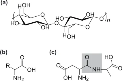
Figure 2. (a) Cellulose is a well-known example of a polysaccharide. It consists of

glucose chains joined by the glycosidic (here –O–) bond. (Cellulose is hydrophilic, but insoluble in water.) (b) An amino acid consists of amine and carboxylic acid groups, with the functional unit (R) diﬀerentiating the diﬀerent kinds. A protein is a series of amino acids joined by peptide bonds. The shading in (c) shows a peptide bond used to join two amino acids, aspartine (left) and alanine (right). Further additions to the peptide would occur at the amine for aspartine, and carboxylic acid for the alanine. The carboxylic group in the aspartine part of the dipeptide is part of the functional group, R

(9)

driven by their chemistry, or whether the underlying physics inherent in large molecules also affects their behaviour. A protein is a series of amino acids joined by peptide bonds, and a polysaccharide is a series of sugar molecules joined together by glycosidic bonds. These are shown in Figure 2. In both cases there are plenty of hydroxyl groups that give rise to the hydrophilicity of the components, as they are sources of hydrogen bonding. Whilst the specific combination of chemical groups or amino acids will interact individually with their environment, the ability of the chain to work as a single entity, as required for its biological function, is driven by the form of the molecule. This is particularly pertinent in the case of proteins, with their naturally folded peptide chains. This type of conformation arises from an energy landscape where one of the most stable low-energy forms is a “marginally compact tube” [43], which has a propensity for generating α-helices and β-sheets, the most important secondary structures in proteins [44]. Furthermore, proteins have been shown to maintain their native folded structure despite amino acid replacement, suggesting that the overall shape and associated crystalline behaviour is at least partially independent of the chemistry of these large biomolecules [45].

Eukaryotes do not have a cell wall, but rather have a membrane. (Plants, however, can have cellulose-based cell walls surrounding the outer membrane.) Their adhesion to surfaces is based on a wider array of adhesion molecules, and these are largely proteins. Their purpose is to ensure that tissue binding is complete, and are not optimized to bind to inorganic surfaces. Since their binding is expected to be to biological tissue, eukaryotic cells are best grown on hydrophilic surfaces in contrast to many prokaryotes, which are best cultured on hydrophobic surfaces.

2. Techniques for the structural investigation of surfaces and interfaces

There are numerous experiments that can be performed to understand the nature of a surface or interface. The questions that arise are based loosely around the information that is needed. An experiment designed to provide morphological information is not likely to be useful if the requirements are chemical information. Furthermore, if the interface is buried, it will be harder to access. It may be necessary to destroy the sample to access that interface, but there are also techniques that can access covered interfaces

in situ, for example by using neutrons. Techniques involving neutrons have their own

(10)

of techniques is subjective, but those considered here have been demonstrated to be important over a number of years.

2.1. Surface analysis techniques

Surface analysis is a phrase often used by veterans of the field specifically to mean photoelectron spectroscopy and secondary-ion mass spectrometry (SIMS). These two techniques would provide chemical information about the surface. Initially, routine high-resolution surface imaging could only be provided by scanning electron microscopy (SEM). Now there is much more choice; photoelectron spectroscopy, SIMS, and SEM are high vacuum techniques and so newer techniques were designed to be somewhat more flexible. The suite of scanning probe techniques allows much greater choice in how samples can be measured, and provides a wide variety of data. Neverthless, if chemical information is needed, photoelectron spectroscopy and SIMS are hard to beat. Infrared techniques, however, can also provide much useful chemical information. There are many reviews concerning surface analysis, but if the reader wishes to see a complete overview, the book edited by Vickerman is to be strongly recommended [46]. Here, with due deference to its position in the history of polymer surfaces, X-ray photoelectron spectroscopy, which is sometimes called electron spectroscopy for chemical analysis, is discussed.

anode crystal

monochromator

sample energy analyzer

vacuum pump focussing lens system

hν

e

-sample input

UHV system

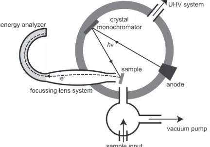
Figure 3. Schematic diagram of a typical XPS set-up. X-rays generated from an

(11)

2.1.1. X-ray photoelectron spectroscopy. The two photoelectron techniques, XPS and

its longer wavelength sibling, ultraviolet (UV) photoelectron spectroscopy (UPS), offer the same operating principle although their uses are slightly different. X-rays or UV are used to eject electrons from the sample. The high-energy X-rays are capable of ejecting core electrons and the resultant information (the energy of these electrons) provides information on the chemical composition and bonding in the material under illumination. UV radiation ejects outermost (valence) electrons form the material under study, and this can enable a better understanding of the electronic structure of the material. UPS is often used for measuring density of states in materials. UPS therefore is mostly (but not exclusively) used for understanding general (bulk) properties and so is of less interest than XPS to those whose primary concern is the surface.

Monochromatic X-rays are generated in a metal source, such as a Kα source of

magnesium or aluminium, in an ultra-high vacuum (UHV) chamber (Figure 3). These X-rays, of energy 1254 eV (Mg Kα) or 1487 eV (Al Kα) are generated in an anode, which

is usually a heated filament. The anode also generates other emission lines as well as the Kα lines that are often used, and so a crystal monochromator can be employed to

remove unwanted lines. (Recent developments include the use of synchrotron radiation in XPS measurements which dispose with the need for a metal source. Furthermore these are tuneable in energy, and here crystal monochromators are particularly helpful.) X-rays are then incident on the sample and they will eject core electrons. X-rays, being uncharged and highly energetic, have a very strong penetration of most samples, but the photoelectrons ejected in the analysis do not travel far. Indeed, it is only the photoelectrons generated very near the surface that can escape the sample and this limits the depth of available information from XPS to no more than 10 nm from the surface, although in most cases it will be less than this.

The energy of the core electrons is different from one element to another, and furthermore bonding changes this energy slightly. The photoelectron energy is measured, and the count rate plotted accordingly. The greater the photoelectron (kinetic) energy is, the less the electron binding energy must be. Alternatively, the count rate can be plotted as a function of binding energy, and an example of this is shown in Figure 4. The binding energy is often plotted in a decreasing energy scale for easy comparison to the kinetic energy. Either way, the binding energy plots are more useful because it is these rather than the kinetic energy plots that can be compared between different X-ray sources. The binding energy is calculated using the simple Einstein energy relation,

Eb=hν−EKE, (1)

where EKE is the kinetic energy of the ejected photoelectron. This relation needs to be

modified to account for the chemical shift due to different bonds (Figure 4) or if the sample is conducting, but it nonetheless encompasses the basic physics.

(12)

2800 284 288 292 1000

2000 3000

Binding Energy (eV)

Counts per second

Carbon scan C–OH C–C

0 200 400 600 800 1000 0

2.104 4.104 6.₁₀4

S

C O

Figure 4. XPS data are ﬁrst obtained with a wide scan to check the presence of

the elements under study. An example survey scan is shown in the inset, along with the locations of the primary carbon, oxygen, and sulfur peaks under study. These scans are low resolution, but for a detailed study, high resolution scans are then performed. The data in the figure are of a C(1S) scan of film of the synthetic metal poly(3,4-ethylene dioxythiophene) (PEDOT) complexed with poly(styrene sulfonate) (PSS) after crosslinking with glycerol. The data are shown as a solid line, and the broken lines show fitting to the data. The fitting allows a clear differentiation between C–OH and C–C bonds. By comparing the relative areas of the peaks associated with the relevant elements and their bonds, the surface compositions of the film can be deduced. These data were used in a study of the water resistance of such films by Rodríguezet al [47]

sulfonate) (PSS), which acts as a dopant and allows processing of the PEDOT in aqueous solution because PEDOT is generally insoluble. It is known that adding high boiling point alcohols such as glycerol [48] or sorbitol [49] to PEDOT/PSS layers can improve performance of polymer devices, but optimizing performance is aided by a detailed knowledge of their structure. The XPS data in Figure 4 show that there is a strong contribution of C–OH bonds in the scan, which is commensurate with a significant amount of glycerol at the surface [47]. The glycerol is not conducting (or semiconducting) and so charge transport between this hole-transport layer (or anode) and the semiconducting layer of the device must be though an insulating layer. Whether this insulating layer improves the quality of the device is not clear, but it is difficult to remove it because thermodynamics (surface energy) control its presence at the surface. It is known from XPS [50] and neutron reflectometry [51] measurements that, without the alcohols, the PSS is located at the surface, so even then the PEDOT is not in contact with the semiconducting layer.

2.1.2. Secondary-ion mass spectroscopy. SIMS is a technique whereby medium-energy

(13)

Ion source

sample

vacuum pump Ion analyzer

sample input

UHV system

Ar+

Mass spectrometer

Detection

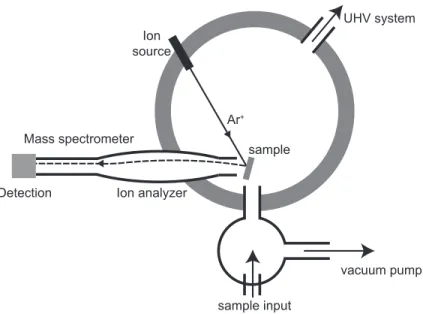
Figure 5. Schematic diagram of a typical SIMS set-up. Charged ions (here Ar+_{) are}

incident on the sample, whereupon they create secondary ions (fragments) in the ﬁlm, which are collected by a lens (ion analyser) and are magnetically selected in a mass spectrometer before detection

charged) such as caesium, oxygen, gallium, and xenon are common — accelerated to an energy of typically 40 keV. This energy is large enough to eject many ions from the film, but, because they are charged, only material in the near surface region can escape, as is also the case for XPS. The typical set-up (Figure 5) is in principle quite similar to an XPS system.

The fragments ejected from the surface are detected in a mass spectrometer, and are differentiated by their mass/charge ratio. Most fragments are singly charged and so the mass/charge ratio simply represents the molecular mass in g/mol of the fragment. Example SIMS data are shown in Figure 6 in which a mixture of poly(l-lactic acid)

(PLLA) and polystyrene is compared with pure films of the two surfaces. (The PLLA is contaminated with polydimethylsiloxane (PDMS), which provides extraneous peaks.) Here, the phase separation of PLLA and polystyrene within the film disrupts the flatness of its surface, creating a film with a topographically structured surface [52]. It has long been known [53] that certain topographically structured surfaces can provide (for reasons not completely understood) a beneficial substrate on which eukaryotic cells can grow and proliferate better than they can on a flat surface [54]. In this work, osteoblast (bone-forming) cells do not grow particularly well on either the polystyrene or PLLA surfaces. PLLA is not particularly hydrophilic; despite its name, it is not an acid: l-lactic acid is polymerized and its carboxylic group is lost in the polymerization

reaction. Nevertheless, the addition of structure by mixing the two polymers improves the surface for cell growth, and the SIMS data provide direct evidence showing that both components are at the film surface.

(14)

0 20 40 60 80 100 120 140 160 180 200 (a)

(b)

(c)

m/Z = 91

polystyrene

poly(ʟ-lactic acid)

mass/charge ratio, m/Z

Figure 6. SIMS data for polystyrene (a) and PLLA (c) ﬁlms. The plots in part (b)

show a mixture of PLLA and polystyrene. The abscissae are in units of g mol−1 _e−1_,

where e is a unit of elementary charge. Using the line marked m/Z = 91, it is clear

that the mixture contains little polystyrene at the surface. Adapted with permission from Limet al. [52]. Copyright (2005) American Chemical Society

the other. In the study of PLLA and polystyrene described here [52], XPS was also performed and a slightly increased polystyrene fraction at the surface was determined than for the SIMS experiments, which helps to add limits to the accuracy of the experiments.

2.1.3. Scanning probe microscopy. The scanning probe microscopies are a suite of

techniques in which a small probe scans across a surface, determining information about the surface topography, strength, chemical structure, or electrical or magnetic properties.

(15)

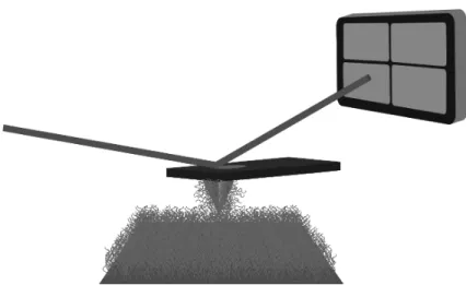
Figure 7. A scanning force microscope consists of a cantilever and tip which is moved

across the surface determining relevant properties of that surface. As the topography changes, surface forces will change and the tip may move in response to these changes. The deflection or movement of the tip can be monitored by the reflection of a laser on the back of the cantilever. This laser beam is detected on a quadrant photodiode. The SFM tip can be modified as necessary. This schematic diagram shows a tip coated with polymer molecules, which is an example of how tribological interactions between different materials can be obtained. Such tip modification allows a control of the interactions with the surface, such as the adhesion, in order to gain a better understanding of surface and material properties

silicon or silicon nitride. (These materials allow for manufacturing accuracy coupled with durability during repeated measurements.) The key components of the SFM are shown in Figure 7. As the tip is moved across the surface, the forces that the surfaces exert on the tip will change. If necessary, a feedback loop can be maintained to keep these forces constant. As the tip rises and falls a map of the surface can be obtained with great (sub-nanometre) precision. For polymer surfaces, dragging a SFM tip across a surface can cause damage to the surface and so intermittent contact is often desirable. In this ‘tapping’ mode the cantilever is driven to a frequency near its resonance and makes contact with the surface only during part of the oscillation. How much of the oscillation is spent in contact with the surface can be controlled. The key requirement is to tap hard enough so that the tip can detect the contours of the surface, but not so hard that it actually indents into soft materials [56].

(16)

provide valuable information about the viscoelastic properties of a polymer surface [59] or material interactions, as schematized in Figure 7, through grafting polymers to the tip surface [60].

Figure 8. A scanning near-ﬁeld optical microscope requires a tapered optical ﬁbre

through which light is directed. The thickness of the fibre is generally between 30 and 100 nm, and the wavelength of the light depends on the information required. If fluorescence imaging is required, then a wavelength appropriate for the fluorescence is required. A map may be taken of the fluorescence (or sometimes simply reflected) light or an image may be taken after absorption through the film, assuming the film is thin enough and the substrate transparent

The resolution of optical microscopy is generally restricted by the Abbe limit of approximately λ/2. This diffraction limit can be circumvented by the use of scanning near-field optical microscopy (SNOM), which is a scanning probe technique in which the probe is an optical fibre brought very close to the sample surface as schematized in Figure 8. The use of SNOM to interrogate polymer surfaces is much less commonly used than SFM, but is nevertheless important, especially in areas such as polymer optoelectronics. Here UV light is passed through the optical fibre and it illuminates the surface. The light may pass through the film as the probe scans across the sample, allowing a transmission image to be built up. Alternatively, scattered light may be detected, in which case a reflection image would be obtained. SNOM, however, is at its most powerful when the incident light from the fibre is used to excite optoelectronic molecules in the film. Through a judicious choice of illuminating light, the molecules in the material fluoresce. Here, an image may be taken locating chemical species in the film by their optical behaviour. This information may be obtained simultaneously with a topography image. The SNOM tip is small enough to be used in the same manner as an SFM tip. It is not ideal, but it is good enough for correlating optical and morphological properties of the film.

Data that exemplify how well SNOM can be used to reveal

informa-tion about a film are shown in Figure 9. Here, a blend of the

opto-electronic polymers poly(9,9-dioctylfluorene-alt-benzothiadiazole) (commonly denoted

(17)

-phenyl-1,4-Figure 9. SNOM can be used to obtain topographical information, and this is

shown (a) for a blend of F8BT and PFB. (b) The light is transmitted through the ﬁlm and collected using an avalanche photodiode (APD). (c) Photoluminescence data from F8BT (obtained in transmission). The use of time-correlated photon counting (TCSPC) allows a determination of the lifetime of the excitation as a function of position, and a map of the photoluminescence lifetime is also shown (d). Reprinted from Cadbyet al. [61], with the permission of AIP Publishing

phenylenediamine) (PFB) is imaged using SNOM [61]. The fluorescence is obtained in transmission in this case after being irradiated with 440 nm light from the SNOM. When mixed with F8BT, PFB emission is suppressed at long wavelengths, allowing a mapping of the the F8BT lifetime as a function of its environment. Here, it is likely that the exciting radiation generates excitons (Coulombically-bound electron–hole pairs) which affect the speed of fluorescence. The more PFB that is present, the slower the luminescence.

Of course, there are many other examples of scanning probe methods. STM, for example has an extremely good resolution, but it is seldom used to study polymer surfaces because it requires conducting and flat substrates in order to function. Further developments have revealed the possibility of parallel processing of polymer surfaces using AFM [62] and SNOM [63, 64]. These techniques have been developed with an eye on memory storage and lithography, and are beyond the scope of this review.

2.1.4. Force spectroscopy Molecular force spectroscopy and single molecule force

(18)

0 20 40 60 80 0 1 2 3 4 5 Distance (nm) Force (nN) (a)

0 20 40 60 80

0 1 2 3 4 5 (d) Distance (nm) Force (nN)

0 20 40 60 80

0 1 2 3 4 5 (c) Distance (nm) Force (nN)

0 20 40 60 80

0 1 2 3 4 5 (b) Distance (nm) Force (nN)

Figure 10. Single molecule force spectroscopy can be used to measure the

adsorption of polymers in different environments. The adsorption of poly(N,N -dimethylacrylamide) (PDMAc) to a silicon substrate depends strongly on its environment. In the case of some environments different conformations are also possible. Here data for PDMAc are shown in water at pH 3. In (a) the polymer has only one contact point with the substrate (as in Figure 1a), but in (b), there are two as noted by the multiple peaks in the retraction curve data shown. (c) A ‘plateau’ in the retraction data shows that the polymer undertakes a ‘pancake’ conformation on the surface, as is also schematized in Figure 1c. (d) A mixture of ‘loops’ into the solution and ‘trains’ on the surface are also possible (Figure 1b). The schematic diagram in each inset indicates the possible conformation of the polymer matching the retraction data; the polymer in the schematic diagram is not to scale with the tip. This figure incorporates previously published data [65]

(19)

Although DLVO theory can be used to describe the interactions measured by force spectroscopy [71, 72, 73], in its basic form it does not account for the interplay between all of the different types of force [74], being solely based on a combination of attractive van der Waals interactions and repulsive double-layer forces [41], and discretion must be used when selecting it for analysis [75, 76]. The extended form of DLVO theory includes some extra features, and can be a better model for forces in a more complex system [77]. However, there is currently no comprehensive theory for bacterial or cellular interactions at a colloidal level, as adhesion in these systems involves a wide range of surface molecules and polymers with different physio-chemical natures as well as contributions from cell elasticity and hydrodynamics [78].

Beyond DLVO theory, there are two alternative models that have been extensively used in the interpretation of force spectroscopy data, and model selection is typically based upon the predicted physical properties of the molecules involved in the interaction. In biological systems, data from flexible polysaccharides are more likely to be fitted using the “freely-jointed chain” (FJC) model, whereas the “worm-like chain” (WLC) model is generally considered more appropriate for DNA and proteins, which are more rigid [79]. The FJC model considers the polymer as comprisingnrigid elements with a length lK (the Kuhn length) that are connected through flexible joints which can rotate freely

in any direction. At low forces, the polymer formation is that of a Gaussian chain, but as force is increased, orientation becomes less random, with preferential alignment oriented along the direction of the external force. Smaller Kuhn lengths correspond to a more flexible polymer [73, 80]. In the FJC model, the force required to stretch a polymer to a length x is given by

Fchain = −kBT

lK L

−1x

lc

, (2)

where kB is the Boltzmann constant, T is the absolute temperature, lc is the contour

length of the portion of the chain that was stretched, and L−1 _{is the inverse Langevin}

function, approximated by the first four terms of its series,

L−1x

lc = 3 x lc + 9 5 x lc 3 +297 175 x lc 5 +1539 875 x lc 7 . (3)

An example of the application of the FJC model in a biological context is the investigation of bacterial surface macromolecules on Pseudomonas putida using SMFS.

It was found that the biopolymers had segment lengths in the range 0.154 – 0.45 nm, but that 65 % of measurements gave a segment length of 0.154−0.20 nm, suggesting that many of the polymers present on the cell surface were highly flexible [80].

In the WLC model, the polymer is considered as a continuous flexible chain of length Lc with a bending stiffness, κ, that can be used to evaluate the persistence length, Lp

by [81]

Lp=

κ kBT

(20)

There is no analytical solution to the WLC model, but the most common approximation is the interpolated WLC [82], given by

F = kBT Lp

"

1 4

1− x

Lc −2

− 1

4+ x Lc

#

, (5)

where F is the elastic restoring force of the chain and x is the end-to-end separation distance. In some cases, the persistence length can be obtained from techniques such as small angle X-ray scattering [83]. The suitability of fixing persistence length can be evaluated by comparing experimental data and the WLC model in a force versus normalized distance plot. Such fixing was appropriate in a study of the swelling of grafted poly(methacrylic acid) (PMAA) layers [84], where Lp was taken as 0.5 nm (it

had been previously determined using small angle X-ray scattering for bulk PMAA [83]), which gave a good fit up to high extension levels, and resulted in greater data fitting accuracy for the contour length, since only one parameter was fitted to the WLC model. This model has also been applied to data obtained when performing force spectroscopy on different bacteria [85, 86, 87]. (Hydrophilic silicon nitride tips do not always give the required peaks and on occasion hydrophobic tips were required to obtain data that could be fitted to the WLC model [88].)

Force spectroscopy is usually performed with an uncoated AFM tip, or an AFM tip coated with gold or a suitable self-assembled monolayer. With such tips, the polymers to be investigated may be in contact with the surface, in which case the process is known colloquially as ‘fishing’. Molecules that cannot be functionalized, for example by

thiolation to react with a gold-coated tip, are generally studied after being picked up on an AFM tip. (It is by no means always necessary to functionalize a molecule in order for it to attach to an AFM tip.) For this to work as a single molecule technique, the polymers must be dilute on the surface, and not entangled with other polymers. The tip can then pick up these molecules and thus measure the interaction with the surface through a retraction curve. This method can be very frustrating as most experiments will not yield a result, because the probe simply makes contact with the substrate. Automation allows for easier experiments, and is becoming increasingly sophisticated [89]. Generally, these fishing expeditions are for biomolecules, which are often very large, making the experiment a little easier. An uncoated AFM tip can be used to characterize dense layers of grafted polymers (brushes), which are tethered by one end to the substrate [90, 91, 92, 93, 94, 95, 96, 97]. By retracting the tip, physisorbed polymers are extended and their length and dispersity in lengths can be assessed.

2.1.5. Quartz crystal microbalance with dissipation A key part of understanding the

interaction of polymers and biopolymers at surfaces relates to adsorption, be it either favourable or unwanted. One method to measure this in both gaseous and liquid environments is to use a quartz crystal microbalance with dissipation (QCM-D). The QCM-D relies on a freely oscillating piezoelectric sensor formed of a thin single crystal quartz (SiO2) disc with electrodes on the upper and lower face (see Figure 11) [98].

(21)

AT-cut quartz crystal (not to scale)

Electrodes Test surface

Direction of flow (dilute test molecule solution)

Direction of flow (wash) A

B C

Figure 11. Schematic diagram of aspects of QCM-D operation. A: when no electric

field is applied, the crystal is under no mechanical stress and the lattice is in a ‘neutral’ position (left). If an electric field of a given direction is applied (middle and right), the crystal is subjected to mechanical stress and deforms, resulting in a lateral shift of the test surface, therefore, the application of an alternating voltage gives rise to sinusoidal oscillations in the crystal. B: during a measurement, the oscillation frequency of the crystal is monitored as test molecules flow across the surface. The amount of adsorbed test molecules is determined using the shift in frequency of crystal oscillation. C: once a layer has adsorbed, the dilute test molecule solution is replaced with a clean solution (a wash, typically a buffer) so that any loosely bound material is removed. The viscoelastic properties of the adsorbed layer can be evaluated from the damping (or dissipation) of the measured crystal oscillations

deformation induces a proportional change in the electric polarization of the material [99]. In the reciprocal effect, application of an external electric field to the piezoelectric material induces mechanical stress in the crystal lattice, resulting in deformation of the crystal. When this crystal is oscillated using a sinusoidal electric field (i.e. an alternating voltage), the fundamental crystal resonance,f0, is dictated by the thickness of the quartz

in the sensor,tq, the shear modulus of the quartz, µq, and its density, ρq, such that

f0 =

1 2tq

s µq

ρq

. (6)

For use in the QCM-D, quartz crystals are typically cut in the AT form, which generates motion lateral to the sensor surface and is relatively immune to temperature-induced fluctuations at room temperature [100]. This mode of operation is referred to as

thickness shear mode.

In its simplest form, prior to a dissipation measurement, the quartz crystal is driven at a selected frequency close to its fundamental mode, setting up oscillations with a constant amplitude. At the start of the measurement the driving voltage is withdrawn, allowing the oscillations to decay naturally to zero. As additional viscoelastic material is adsorbed the rate of decay of oscillations will be ‘damped’ (dissipation) and the

(22)

sequentially flowing them across the sensor (generally interspersed with flow of a wash buffer to remove any non-adherent molecules in between tests, see Figure 11),

acontinuous resonance mode can be used, where the driving electric field is maintained

throughout and relative shifts in the crystal frequency (∆f) are measured [100]. The QCM-D can therefore be used to track adsorption of molecules and biomolecules to the sensor surface [104]. In addition to monitoring the amount of adsorbed material, it can also provide information about the viscoelasticity of the adsorbed molecules, and is therefore useful for testing for adsorption barriers [105].

The mass of adsorbed material can be evaluated using the Sauerbrey model, which neglects viscoelastic effects, and assumes a rigid adsorbed layer. According to the Sauerbrey equation [106], the frequency change ∆f in the piezoelectric crystal due to the adsorbed mass ∆m is given by

∆f =−f03/2 s

ηlρl

πρqµq

, (7)

where ρl and ηl are the density and viscosity of the fluid, respectively. The adsorbed

mass is determined from the changes in viscosity. Masses given include that of any water that is bound or coupled to the surface. This model is appropriate if changes in energy dissipation are small and the adsorbed layer is relatively rigid. The use of an unmodified Sauerbrey equation for soft or viscoelastic films can lead to an underestimate of adsorbed mass [102].

Dissipation data may also be obtained to allow analysis of viscoelastic effects; if the material is tightly-bound and rigid, then minimal dissipation modification would be expected, so the greater the dissipation change for a unit change in gained mass, the more viscoelastic the adsorbed material is [107]. This increase in dissipation can be caused by two things: a more viscoelastic molecule or a poorly attached layer causing dissipation due to friction associated with moving out of synchronization with the resonating crystal. If there is doubt, the origin of the dissipation can be established from thickness data obtained by methods such as ellipsometry; if the change is related to molecule properties, the layer should be thicker, whereas if it is due to loosely bound material there should be a thinner layer. One might argue that ellipsometry is as versatile a method, but QCM-D offers much higher sensitivity and has been shown to detect single molecule binding events, which is beyond the capability of any ellipsometer. However, the benefits of combining QCM-D with other surface analysis techniques within a single system (such as ellipsometry [105] or localized surface plasmon resonance [108]) is not without merit, as this enables additional information to be obtained simultaneously through the same sample and measurement platform.

2.2. Depth profiling and buried interfaces

Techniques that allow us to understand the variation of a particular quantity as a function of distance from an interface are known as depth-profiling experiments. The

(23)

and particularly so in the case of buried interfaces. Experiments in aqueous solution are important for biological samples; these are often not of interest in a dry state. To image buried interfaces is not easy. If the interfaces are in a low viscosity liquid environment then scanning probe techniques can be used, assuming the liquid will not damage the apparatus, but other techniques described above such as SIMS and XPS are inappropriate due to their vacuum requirements. For these reasons most buried interfaces can only be effectively studied in one dimension by depth profiling.

2.2.1. Reflectometry. Perhaps the most powerful depth profiling technique is that of

neutron reflectometry [110, 111, 112, 113]. Here, a beam of neutrons is incident on the sample to be studied. The neutrons may be monochromatic, or as is more often the case, pulsed with a spectrum of wavelengths in the Ångstrom range. The very short wavelength of the neutrons, and for X-rays when considering the similar technique of X-ray reflectometry [111], allows for an extremely good depth resolution. Neutrons are versatile because they are only weakly scattered by many materials, which means that they can traverse large distances before reaching the interface in question. Water, unfortunately, does scatter neutrons, but it is not necessary to send neutrons through a bath of water in order to reach the interface to be studied; neutrons can interrogate the interface in question by passing through many substrates with little loss of intensity (e.g. silicon). Contrast in neutron reflectometry experiments is most often achieved by selective deuteration of one of the components in the film. If two polymers are mixed, then one of them would normally be deuterated. In aqueous environments it is generally advantageous to use heavy water, because of the extensive scattering of neutrons by normal water (H2O). Although it is possible to account for this scattering by careful

analysis, it detracts from the quality of the data. The use of heavy water does make some biopolymer experiments difficult to consider, because often H/D exchange occurs in biopolymer solutions, particularly in the case of certain proteins [114]. Nevertheless, neutron reflection has been used in many experiments to study biomacromolecules, and an example is shown in Figure 12 for the rather shorter chain molecule, mycolic acid [109]. Many of the advantages of neutron reflectometry also apply to X-ray reflectometry. X-ray scattering techniques work best when there is a heavy element present in the sample, as these provide contrast. This restriction is not prohibitive, however, and X-rays are also useful for the characterization of the surface of thin films. X-ray reflection is, however, not viable for the study of buried liquid interfaces. Nevertheless X-rays are less expensive than neutrons and are available in laboratory apparatuses. Which technique is used depends therefore on a variety of different parameters but the information obtained is broadly similar. By way of example, the use of X-ray reflectometry to study the structure of films to explain adhesive behaviour [115] provides information broadly comparable to studies used for similar purposes with neutrons [116, 117, 118, 119, 120].

2.2.2. Ion beam analysis. Other depth profiling techniques require the use of ions to

(24)

0.00 0.05 0.10 0.15 –6

–4 –2 0

pD 3.0 pD 7.0 pD 10.0

Momentum transfer, Q (Å−1)

Reflectivity, log

10

(

R

)

0 2 0 4 0 6 0 0

2 4 6

pD 3.0 pD 7.0 pD 10.0

SLD (10

−6 Å −2)

Depth (nm)

(a)

0 10 20 30 40 50

0.0 0.2 0.4 0.6 0.8 1.0

pD 3.0 pD 7.0 pD 10.0

Depth, z (nm)

MA volume fraction,

φ

(b)

Figure 12. Mycolic acid is a biosurfactant associated with mycobacteria. Here,

neutron reflectometry data are shown for an aqueous solution mycolic acid from the human tuberculosis bacterium with the carboxylic acid group exposed. The neutron reflectometry data are shown in (a), and in the inset, the scattering length density profile is displayed. This scattering length density profile is from a silicon substrate (z = 0), and attains a rather large value of 6.48 Å−2 at large depths; this scattering

length density corresponds to heavy water. There is a clear extension of the acid at pD 10, but not much change between pD 3.0 and 7.0. (Note the use of pD, rather than pH.) The volume fraction proﬁle of the mycolic acid is extracted and shown in (b). The inset in (b) shows the chemical structure ofα-mycolic acid, which is one of

a mixture of mycolic acids contained with the sample studied here. Reprinted from Zhanget al. [109]. Copyright (2010), with permission from Elsevier

(25)

Techniques falling under the umbrella of ion beam analysis do not include dynamic SIMS, which is more a mass spectrometry technique. Ion beam analysis generally requires a means of monitoring the energy of ions as they exit a film that was interrogated by a beam of ions, which may or may not be the same as those incident on the film. With ion beam analysis, different techniques allow for a very flexible approach. The best known ion beam technique is Rutherford Backscattering (RBS) [123, 124]. Here a

beam of ions (usually α-particles) of energy of the order of 3 MeV is incident on the sample. These ions have a small collision cross section (recall the revelations about the interaction of α-particles with gold and other metals in the original experiments of Geiger and Marsden [125]) and so it takes a relatively thick film, up to 10 µm, to stop them all. By measuring the energy of the detected α-particles, one can determine the depth in the film at which the backscattering event took place. (The energy loss of α-particles in different materials is tabulated [126].) With these measurements, a depth-profile can be constructed. RBS is less commonly used in soft matter research, because there are relatively few polymeric systems that contain the heavy elements required for good RBS data, although some studies have been performed [127], and other studies have been concerned with the location and behaviour of heavy elements in polymer matrices [128, 129, 130]. Figure 13 shows an example of such data. Heavy elements can, however, also be added as markers to define the movement of polymers [131], or to stain an individual component of a mixture [132]. RBS, like SIMS and XPS, is restricted by a vacuum requirement because the α-particles will be scattered in air. Nevertheless, developments have been made to allow their use to study samples in different environments [133, 134], although their application is away from the areas concerned in this review.

Ion beam techniques more commonly used for the study of thin polymer films includenuclear reaction analysis(NRA) andforward recoil spectrometry(FReS) because

they both allow a means of determining the profile of light elements in the sample, and as such are very often complementary to neutron reflectometry. (Neutron reflectometry provides excellent resolution, but because the information obtained is in Fourier space, it is often useful to start with depth profiling information which can provide the initial conditions for fitting the reflectivity data.) FReS, sometimes called elastic recoil detection analysis (ERDA) is a relative of RBS. In RBS the incident α-particle recoils from the nucleus. In FReS the energy of the deflected α-particle is not needed, but rather the energy of protons and deuterons ejected from the nucleus are measured. Their energy is obtained using kinematics, just as in RBS; here however the nucleons

are forward scattered, as opposed to the backscattering in RBS. Backscattering means

that the incident particles recoil on hitting the nucleus and forward scattering means that the ejected particles are sent away from the initial beam. The forward scattering is a consequence of the protons and deuterons being a lighter mass than the incident α-particles. An advantage of FReS is its ability to determine the volume fraction-depth profile of both deuterated and non-deuterated components of a film.

(26)

Figure 13. Rutherford Backscattering data from nanorods of titanium dioxide in a

matrix of polystyrene. The TiO2 nanorods are allowed to diﬀuse into the polystyrene

at 190◦ _{and the diﬀusion can be modelled using Fick’s second law, from which a}

diffusion coefficient may be obtained. These measurements in which a heavy element such as titanium is used are ideal for RBS because of the high scattering cross section. In such experiments the excellent resolution afforded by reflectometry is not needed and furthermore, the large length scales associated with interdiffusion of this nature are usually inaccessible with reflectometry techniques, which work better with sharper interfaces. Adapted with permission from Choiet al. [130]. Copyright (2015) American Chemical Society

volume fraction-depth profile of a given component in a film. There are many different variants of NRA, but the most popular for the determination of the structure of polymer films is3_{He NRA. Here a mono-energetic beam of}3_He+_{ions is incident on the film. The}

energy of the ions is typically ∼ 1 MeV, and at about this energy 3_He++ _{(the other}

electron is immediately lost on impact with the film) reacts with deuterons to yield a lithium compound nucleus, which quickly decays to create an α-particle and a proton, as well as about 18.5 MeV of energy; the reaction is very exothermic. The 3_{He nucleus}

loses energy as it penetrates the sample, and this changes the reaction kinetics, altering the energy of the proton and α-particle produced. Either the proton or α-particle can be detected, and their energy allows a calculation of the position in the sample at which the reaction took place. (How well 3_{He is stopped by matter is tabulated [126], just as}

for α-particles, so one can work out the energy that these nuclei must have had at a certain depth in the sample.)

3. Physical phenomena at surfaces and interfaces

(27)

domains. These domains seek to merge with other, similar, domains to form bigger spheres, reducing their surface to volume ratio. However, even circular structures are not necessarily stable, because of the difference in pressure across a surface (the Laplace pressure) and the disjoining pressure caused by having different material phases in contact.

The interface between two polymer components tells us about the competition between entropy and enthalpy, and thus allows us to dissect the interfacial energetics of a particular set of materials. The structure of a blend or mixture of polymers at a free or fixed interface also will be different to that in the middle of the film. These interactions can lead to stratified or segregated structures, where polymers wet the surface. Sometimes the film will simply dewet its surface. Finally, polymer films can be controlled by chemically attaching them to the surface. These are known as polymer brushes, and have many applications in terms of controlling film stability, adhesion, colloidal stabilization, cell culture, and even in all-polymer electronic devices.

The structure and morphology of polymer blend films has been intensively studied over the past 25 years, and developments have been made with specific applications in mind, such as the use of blends in optoelectronic devices. From a more general perspective the study of the formation of films during drying is an area of research where experimental developments have allowed quantitative studies to take place. Although these subjects will be covered here; films of one homopolymer have been used as a vehicle for fundamental studies of basic phenomena, such as crystallization, and this will also be addressed. Finally, the use of films as actuators will be presented, highlighting the role of brushes in this new area of research.

Perhaps the area of polymer thin film research that has received the most attention is dewetting and related phenomena. The stability of films and coatings is important in many areas of technology, and so we consider developments in this area first.

3.1. Wetting and dewetting

The stability of most polymer films can be characterized by the use of contact angle experiments (Figure 14), which typically give a description of the free energy of a sample compared to that of water: hydrophilic surfaces are those where the interfacial energy of the water-solid contact is below the free surface energy of the solid, whereas hydrophobic surfaces exhibit the opposite relationship, with the solid having the smaller surface energy, or tension.

In systems where the contact angle does not vary with time and an equilibrium,

static contact angle is attained, the surface energies in the system can be related to the

contact angle θ, by

γLVcosθ =γSV−γSL, (8)

where γLV, γSV, and γSL are the liquid–vapour, surface–vapour and surface–liquid,

(28)

θ

γ

_LV

γ

_SL

γ

_SV

Figure 14. The contact angle of a liquid is a balance between the surface and

interfacial energy of the diﬀerent components: γLV for that between the liquid and

its vapour;γSV, that between the solid and the liquid vapour; andγSLfor the interface

between the solid and liquid phases. For experiments in which the liquid is water, a contact angle,θless than 90◦ _{denotes a hydrophilic surface; when}_{θ >}₉₀◦_{, the surface}

is hydrophobic; and forθ >150◦, the surface is usually referred to as superhydrophobic

rigid, insoluble, chemically homogeneous, and unreactive) and it takes its name (the Young equation) from Young’s work in the early 19th _{century [135].}

The contact angle is particularly relevant for biomaterials, where very hydrophilic surfaces tend to be associated with good biocompatibility. The ability of a material to remain solvated in the presence of other macromolecules means that that surface is less likely to be fouled. Wettability of surfaces is also a strong indicator of adsorption, with profound consequences for cell growth and protein fouling [136]. This can be characterized through instability in the temporal behaviour of the contact angles, with changes in droplet volume (in conditions with minimal evaporation) either due to droplet absorption, spreading, or a mixture of the two [137]. In the case of suchdynamic contact

angle measurements, wetting of a hydrophilic surface is associated with an advancing

water contact angle [138], and dewetting of a hydrophobic surface with a receding contact angle [139]. Absorption is not always relevant because it requires the surface to have some limited solubility in water but can be considered in terms of a decrease in droplet basal area along with a decrease in volume, whereas spreading results in an increase in basal area.

Both static and dynamic contact angle measurements play an important role in the characterization of polymer surfaces for use in various applications, ranging from the medical field, in terms of reducing harmful biofouling or encouraging native cell growth on implants [140, 141]; to optometry and contact lens anti-fouling properties [142, 143, 144], wetting agents [145] and in-built drug delivery [146, 147], to the replacement of petrolium-based polymers with biopolymers which are able to replicate their hydrophobic properties [148].

Although the water contact angle is an important characterization tool for biomaterial surfaces and for surfaces that may be placed in contact with water, it is less useful for understanding whether or not a film is stable. The Young equation (Equation 8) also allows prediction of film stability, and can be used to define stability through the spreading coefficient,

S=γSV−(γSL+γLV). (9)

(29)

preferentially coat that surface; i.e. the film willwet the surface. Similarly, whenS <0, the film will be unstable on the surface and will want to dewet the substrate.

The stability of thin polymer films depends predominantly on long-range interactions between the film and its environment, and these generally take the form [41]

Wj(x) =− Aijk

12πx2, (10)

whereWjrepresents the interaction energy of two parallel and planar semi-infinite media

(i and k) separated a distance x by a medium j. The parameter Aijk is known as the

Hamaker constant and depends on all three materials, although approximations can be made to calculate Aijk from Hamaker constants of the component materials, Aii where

the two (identical) components are separated by vacuum. A more detailed (Lifshitz) treatment relies on the dielectric properties of the different layers [41].

10 100

PMMA thickness (nm)

Polystyrene thickness (nm)

Figure 15. Phase diagram for the dewetting of a bilayer of PMMA on polystyrene

on a silicon substrate. Filled diamonds represent the instability of the upper PMMA layer on a stable polystyrene film; circles the reverse situation, whereby the PMMA layer is stable, with a broken polystyrene film beneath it. Both layers can be destroyed through thermal nucleation (squares). Triangles represent data for films that could not be attributed to a particular structure. The upper left shading represents regions of the film for polystyrene, and the lower right triangular shaded region is for stable PMMA films. The thin dashed lines represent uncertainty in the limits on the stability of the PMMA films. Data used with permission from de Silvaet al. [149]

(30)

Whilst varying the thickness of the layers allows the interaction between the films to be tailored to control stability, a film may create its own interface potential that can strongly affect film stability. Diblock copolymers with each block containing similar chain sizes will order to form a stacked (lamellar) structure, with the block that lowers the interfacial energy segregating to the substrate and the block that lowers the surface energy segregating to the surface. These blocks may be the same, or different blocks may segregate to the different interfaces. A lamellar structure will only form if the ratio of the chain lengths in each block is close to unity and the blocks are immiscible. A surface will perturb the structure, and even if the two blocks are miscible, they will order close to the surface, with the amount of order decaying with distance from the substrate. This creates an oscillating interface potential the minima and maxima of which become less pronounced with distance from the substrate, which permits a situation where the melt above a residual layer ordered at the substrate may dewet [150]. Here the dewetting of a diblock copolymer containing immiscible blocks (poly(2-vinylpyridine) and polystyrene) occurs to allow a disordered state to exist close to the substrate whilst retaining a lamellar structure at the air interface, and can proceed when the energy driving ordering is weak. However, the differing diblock copolymer film thicknesses at which this dewetting may occur result in discrete contact angles, even though the composition of the film is the same.

Other recent challenges in dewetting concern the effect of the preparation of thin films on their subsequent behaviour. The microscale morphology of films, and the conformation of polymers within the structures produced by common techniques such as spin coating, are not expected to be at equilibrium. Indeed, there are no methods currently available that routinely produce films at equilibrium. Part of the reason for the resultant out-of-equilibrium structures is the rapid quench in many drying processes, but also there will be a contribution due to the presence of solvent within the polymer film after casting. Later evaporation of the solvent leads to residual stresses within the film, which in many cases is already glassy. There is a clear effect on the distribution of holes in such films, as has been determined by simple optical microscopy experiments [151], where it was observed that the longer the films have to relax, the fewer the number of holes that appeared in the dewetted film (Figure 16).

(31)

0 20 40 60 80 100 120 140 0

0.04 0.08 0.12 0.16 0.2 0.24

Ageing time (s)

Maximum number of holes / mm

2

0 1000 2000 3000 4000 5000 0

0.04 0.08 0.12 0.16 0.2 0.24

Time (s)

Holes / mm

2

2.25 h

6.5 h

8 h

12 h

34 h

72 h

108 h

134 h

(a)

(b)

Figure 16. (a) The areal density of holes,N, as a function of time at125◦C for 40 nm

thick polystyrene ﬁlms after being aged at50◦_{C for diﬀerent times. The maximum hole}

density (per104_µm2),_N_maxfor each sample is reached in about 100 s. (b)_N_max as a

function of ageing time for similar polystyrene type of ﬁlms stored at50◦_{C for various}

times. The insets show some typical corresponding optical micrographs (310_×230

µm2_{). The solid line is a ﬁt to the data with a decaying exponential. Adapted with}

of relaxing rather quickly, indicating that they were closer to equilibrium than shorter polymers of the same chemical structure [158].

(32)

was that of a viscous fluid, with a behaviour dominated by slippage. Slippage in itself has been of some considerable interest in dewetting since systematic SFM experiments were able to follow the shape of the rim during dewetting from a deformable polymer interface [160]. The shape of the rim is important, because it can reveal much about the viscoelastic behaviour of polymers. An initial simple approach to dewetting proposed that the gain in surface energy by the dewetting process is translated into the kinetic energy of the dewetting polymer [161], which is only valid for a low viscosity liquid on a non-deformable substrate. For deformable and liquid substrates, the dewetted polymer accretes into a rim, whose shape depends strongly on the viscosity of that polymer, as well as that of the substrate. Here friction can also be important, and this will increase with the size of the rim, which forces the dewetting speed to decrease. Of course, if friction is limited, then the dewetting polymer may well slip at the interface. Its tendency to slip depends on how much the chains of the two layers can interpenetrate; generally, interpenetration or interdigitation is limited, because otherwise the layers would be compatible and the films stable. Certainly, it has been clearly demonstrated that dewetting proceeds more rapidly on surfaces with less slippage, and hence less friction [162, 163].

Applications of dewetting in various nanotechnologies are still being developed but the basic science must be fully understood before real progress can be obtained. It is expected that dewetting can be advantageously used in a number of new areas, in particular those where patterning is important [164]. For example, the use of selective dewetting to align electrode materials has been developed, a route that may be easily applied using ink-jet printing [165, 166]. Microcontact printing and other patterning techniques can be used to control the structure of films [167, 168, 169, 170, 171]. Although the fundamental science of dewetting is still proceeding, the development of technologies based on dewetting probably has slowed somewhat in the past decade and it is perhaps likely that a new breakthrough is needed to reignite the field.

3.2. Blends in optoelectronic devices

Ever since the observation of electrical conductivity in excess of 10 kS/m in doped polyacetylene was reported in 1977 [172], there has been interest in developing polymers for electronics applications. Although conducting polymers, and PEDOT in particular, have applications in various areas from antistatic films [173], transparent electrodes [173, 174], and bioelectronics [175, 176], it is in the area of polymeric semiconductors where the greatest interest is to be found. Interfaces in polymer electronics are crucial for numerous reasons because they influence and direct morphological behaviour, and can also influence the electronic properties directly.

(33)

exciton [37]. This exciton may decay back to an electron and hole, or it may radiatively decay, giving off a visible photon. (The band gap is the primary determinant of the wavelength of the light emitted.) Clearly for an optimal LED, the amount of excitons giving off light must be maximized, and the number of holes and electrons making it to the opposite electrode without giving off light must be minimized. A parameter by which a device may be controlled is the ratio of the two components in the polymer layer. Other aspects, such as the contact between the layer and electrodes, and the benefits of injection layers will not be discussed here, but they are important considerations [177], and they also affect polymeric photovoltaic cells and transistors [37, 178].

0.0 0.2 0.4 0.6

Volume fraction d−F8,

φ

Depth, z (nm)

0 40 80 120

0.0 0.2 0.4 0.6

Volume fraction d−F8,

φ

(a)

(b)

Figure 17. 3_{He NRA data and simulations (volume fraction-depth proﬁles) for a}

blend of 50% F8 and 50% F8BT by volume cast from (a) toluene and (b) chloroform. The peak in the data atz = 0 for the toluene-cast ﬁlm indicates that F8 (the

d-indicates that the F8 is partially deuterated, for contrast in the ion beam experiment) preferentially segregates to the air interface, with an F8BT-rich region immediately behind it. There is much less structure visible in the chloroform-cast ﬁlm. The non-sharp interfaces atz= 0and_z_≈100nm are due to the resolution of the experiment.

Such resolution effects mask the volume fraction of d-F8 at the surface of the film in the data for the toluene-cast film, which could be close to unity. Taken from Higgins