A command for fitting mixture regression models for bounded dependent variables using the beta distribution

dependent variables using the beta distribution

.

White Rose Research Online URL for this paper:

http://eprints.whiterose.ac.uk/129553/

Version: Published Version

Article:

Gray, L.A. orcid.org/0000-0001-6365-7710 and Alava, M.H.

orcid.org/0000-0003-4474-5883 (2018) A command for fitting mixture regression models

for bounded dependent variables using the beta distribution. Stata Journal, 18. pp. 51-75.

ISSN 1536-867X

[email protected] https://eprints.whiterose.ac.uk/ Reuse

Unless indicated otherwise, fulltext items are protected by copyright with all rights reserved. The copyright exception in section 29 of the Copyright, Designs and Patents Act 1988 allows the making of a single copy solely for the purpose of non-commercial research or private study within the limits of fair dealing. The publisher or other rights-holder may allow further reproduction and re-use of this version - refer to the White Rose Research Online record for this item. Where records identify the publisher as the copyright holder, users can verify any specific terms of use on the publisher’s website.

Takedown

If you consider content in White Rose Research Online to be in breach of UK law, please notify us by

Editors

H. Joseph Newton

Department of Statistics Texas A&M University College Station, Texas [email protected]

Nicholas J. Cox

Department of Geography Durham University Durham, UK

[email protected]

Associate Editors

Christopher F. Baum, Boston College

Nathaniel Beck, New York University

Rino Bellocco, Karolinska Institutet, Sweden, and University of Milano-Bicocca, Italy

Maarten L. Buis, University of Konstanz, Germany

A. Colin Cameron, University of California–Davis

Mario A. Cleves, University of Arkansas for Medical Sciences

Michael Crowther, University of Leicester, UK

William D. Dupont, Vanderbilt University

Philip Ender, University of California–Los Angeles

James Hardin, University of South Carolina

Ben Jann, University of Bern, Switzerland

Stephen Jenkins, London School of Economics and Political Science

Ulrich Kohler, University of Potsdam, Germany

Frauke Kreuter, Univ. of Maryland–College Park

Peter A. Lachenbruch, Oregon State University

Stanley Lemeshow, Ohio State University

J. Scott Long, Indiana University

Roger Newson, Imperial College, London

Austin Nichols, Abt Associates, Washington, DC

Marcello Pagano, Harvard School of Public Health

Sophia Rabe-Hesketh, Univ. of California–Berkeley

J. Patrick Royston, MRC CTU at UCL, London, UK

Mark E. Schaffer, Heriot-Watt Univ., Edinburgh

Philippe Van Kerm, LISER, Luxembourg

Vincenzo Verardi, Universit´e Libre de Bruxelles, Belgium

Ian White, MRC CTU at UCL, London, UK

Richard A. Williams, University of Notre Dame

Jeffrey Wooldridge, Michigan State University

Stata Press Editorial Manager Lisa Gilmore

Stata Press Copy Editors

Adam Crawley,David Culwell, andDeirdre Skaggs

TheStata Journalpublishes reviewed papers together with shorter notes or comments, regular columns, book

reviews, and other material of interest to Stata users. Examples of the types of papers include 1) expository papers that link the use of Stata commands or programs to associated principles, such as those that will serve as tutorials for users first encountering a new field of statistics or a major new technique; 2) papers that go “beyond the Stata manual” in explaining key features or uses of Stata that are of interest to intermediate or advanced users of Stata; 3) papers that discuss new commands or Stata programs of interest either to a wide spectrum of users (e.g., in data management or graphics) or to some large segment of Stata users (e.g., in survey statistics, survival analysis, panel analysis, or limited dependent variable modeling); 4) papers analyzing the statistical properties of new or existing estimators and tests in Stata; 5) papers that could be of interest or usefulness to researchers, especially in fields that are of practical importance but are not often included in texts or other journals, such as the use of Stata in managing datasets, especially large datasets, with advice from hard-won experience; and 6) papers of interest to those who teach, including Stata with topics such as extended examples of techniques and interpretation of results, simulations of statistical concepts, and overviews of subject areas.

TheStata Journalis indexed and abstracted byCompuMath Citation Index,Current Contents/Social and

Behav-ioral Sciences,RePEc: Research Papers in Economics,Science Citation Index Expanded(also known asSciSearch),

Scopus, andSocial Sciences Citation Index.

For more information on theStata Journal, including information for authors, see the webpage

http://www.stata.com/bookstore/sj.html

Subscription rateslisted below include both a printed and an electronic copy unless otherwise mentioned.

U.S. and Canada Elsewhere

Printed & electronic Printed & electronic

1-year subscription $124 1-year subscription $154

2-year subscription $224 2-year subscription $284

3-year subscription $310 3-year subscription $400

1-year student subscription $ 89 1-year student subscription $119

1-year institutional subscription $375 1-year institutional subscription $405 2-year institutional subscription $679 2-year institutional subscription $739 3-year institutional subscription $935 3-year institutional subscription $1,025

Electronic only Electronic only

1-year subscription $ 89 1-year subscription $ 89

2-year subscription $162 2-year subscription $162

3-year subscription $229 3-year subscription $229

1-year student subscription $ 62 1-year student subscription $ 62

Back issues of theStata Journalmay be ordered online at

http://www.stata.com/bookstore/sjj.html

Individual articles three or more years old may be accessed online without charge. More recent articles may be ordered online.

http://www.stata-journal.com/archives.html

TheStata Journalis published quarterly by the Stata Press, College Station, Texas, USA.

Address changes should be sent to the Stata Journal, StataCorp, 4905 Lakeway Drive, College Station, TX 77845, USA, or emailed to [email protected].

® ®

Copyright c2018 by StataCorp LLC

Copyright Statement: TheStata Journaland the contents of the supporting files (programs, datasets, and help files) are copyright cby StataCorp LLC. The contents of the supporting files (programs, datasets, and help files) may be copied or reproduced by any means whatsoever, in whole or in part, as long as any copy or reproduction includes attribution to both (1) the author and (2) theStata Journal.

The articles appearing in theStata Journalmay be copied or reproduced as printed copies, in whole or in part, as long as any copy or reproduction includes attribution to both (1) the author and (2) theStata Journal.

Written permission must be obtained from StataCorp if you wish to make electronic copies of the insertions. This precludes placing electronic copies of theStata Journal, in whole or in part, on publicly accessible websites, fileservers, or other locations where the copy may be accessed by anyone other than the subscriber.

Users of any of the software, ideas, data, or other materials published in theStata Journalor the supporting files understand that such use is made without warranty of any kind, by either theStata Journal, the author, or StataCorp. In particular, there is no warranty of fitness of purpose or merchantability, nor for special, incidental, or consequential damages such as loss of profits. The purpose of theStata Journalis to promote free communication among Stata users.

TheStata Journal(ISSN 1536-867X) is a publication of Stata Press. Stata, , Stata Press, Mata, ,

A command for fitting mixture regression

models for bounded dependent variables using

the beta distribution

Laura A. Gray

School of Health and Related Research Health Economics and Decision Science

University of Sheffield Sheffield,UK

[email protected]

M´onica Hern´andez Alava School of Health and Related Research Health Economics and Decision Science

University of Sheffield Sheffield,UK

[email protected]

Abstract. In this article, we describe the betamix _{command, which fits}

mix-ture regression models for dependent variables bounded in an interval. The model is a generalization of the truncated inflated beta regression model introduced in Pereira, Botter, and Sandoval (2012, Communications in Statistics—Theory and Methods 41: 907–919) and the mixture beta regression model in Verkuilen and Smithson (2012,Journal of Educational and Behavioral Statistics37: 82–113) for variables with truncated supports at either the top or the bottom of the distri-bution. betamix _{accepts dependent variables defined in any range that are then}

transformed to the interval (0,1) before estimation.

Keywords:st0513, betamix, truncated inflated beta mixture, beta regression,

mix-ture model, cross-sectional data, mapping

1

Introduction

Continuous response variables that are bounded at both ends arise in many areas. De-pendent variables measuring proportions, ratios, and rates are common in the empirical literature. They are often limited to the open unit interval (0,1), but in many cases, values in both boundaries are not only possible but appear with high frequency. Ap-plications where the variables are bounded in alternative intervals linearly transform the dependent variable to the (0,1) interval. Some examples include modeling the rates of employee participation in pension plans (Papke and Wooldridge 1996), the per-centage of women on municipal councils or executive committees (De Paola, Scoppa, and Lombardo 2010), an index measuring central bank independence (Berggren, Daun-feldt, and Hellstr¨øm 2014), the proportion of a firm’s total capital accounted for by its long-term debt (Cook, Kieschnick, and McCullough 2008), quality adjusted life years (Basu and Manca 2012), and the score of reading accuracy (Smithson and Verkuilen 2006).

Modeling variables bounded at both ends presents several problems. The usual linear regression model is not appropriate for bounded dependent variables, because the predictions of the model can lie outside the boundary limits. A common

solu-c

tion is to transform the dependent variable so that it takes values in the real line and then use standard regression models on the transformed dependent variable. How-ever, this approach has an important limitation in that it ignores that the moments of the distribution of a bounded variable are related; as the mean response moves toward a boundary value, the variance and skewness of the variable will tend to de-crease and inde-crease, respectively. Fractional response models (Papke and Wooldridge 1996, 2008) and models based on the beta distribution have been suggested as alterna-tives (Paolino 2001; Kieschnick and McCullough 2003; Ferrari and Cribari-Neto 2004; Smithson and Verkuilen 2006). Fractional response models (Papke and Wooldridge 1996; 2008) assume that the dependent variable takes values in the unit interval [0,1]. Papke and Wooldridge (1996) specified a functional form for the conditional mean of the dependent variable and proposed the use of a quasilikelihood procedure to estimate the parameters. These models are very useful if the main interest is in the conditional mean of the dependent variable and, if the conditional mean is correctly specified, the parameter estimates are consistent.

The standard beta regression model (Paolino 2001; Ferrari and Cribari-Neto 2004; Smithson and Verkuilen 2006) assumes that the dependent variable is continuous in the open unit interval (0,1). Unlike the fractional response model described above, the beta regression model assumes a distribution for the dependent variable condi-tional on the covariates, and its parameters are estimated using maximum likelihood. A drawback of this model is that distributional misspecification leads to inconsistent parameter estimates. However, it is more suitable if the interest is in the whole dis-tribution. This model has been generalized to allow for values at either boundary or both boundaries by adding a degenerate distribution with probability masses at the boundary values (Cook, Kieschnick, and McCullough 2008; Ospina and Ferrari 2010, 2012b; Basu and Manca 2012). Pereira, Botter, and Sandoval (2012, 2013) extend the framework to model variables such as the ratio of the unemployment benefit to the maximum benefit. This ratio can take the value of zero (if the person is not eligible) or any real number in the interval (τ,1), where τ is the minimum benefit. The ra-tio is also likely to have positive probabilities at the values τ and at 1. This model was termed the truncated inflated beta distribution. The model is a mixture of the beta distribution in the interval (τ,1) and the trinomial distribution with probabil-ity masses at 0,τ, and 1. A related strand of the literature extends the standard beta regression model to allow for mixtures ofC-components of beta regressions. This exten-sion is helpful when the distribution of the dependent variable presents characteristics that cannot be captured by a single beta distribution such as multimodality. Allowing for mixtures can help overcome misspecification problems in the conditional distribu-tion of the dependent variable. Some examples of mixtures of beta distribudistribu-tions are found in Ji et al. (2005), Verkuilen and Smithson (2012), and Kent et al. (2015). In Gray, Hern´andez Alava, and Wailoo (Forthcoming), we combine these extensions into a single model to address the problems of modeling health-related quality of life (HRQoL) in health economics.1

In this article, we present the commandbetamix, which can be used to fit mixture regression models for dependent variables that are bounded in an interval and can have truncated supports either at the top or at the bottom of the distribution. It extends one of the parameterizations of the community-contributed commandsbetafit and zoib

and the Stata command betaregin several directions.2 _{First, it generalizes them to} mixtures of beta distributions, allowing the model to capture multimodality. Second, it allows the user to model response variables that have a gap between one of the boundaries and the continuous part of the distribution. Third, it can deal with positive probabilities at either boundary or both boundaries and at the truncation point. Fourth, there is no need to manually transform response variables defined in intervals other than (0,1), becausebetamixwill transform the dependent variable using the supplied options.

This article is organized as follows: section 2 gives a brief overview of the model; section 3 describes the betamixsyntax and options, including the syntax forpredict; section 4 illustrates the syntax of the command and the interpretation of the model using a fictional dataset; and section 5 concludes.

2

A general beta mixture regression model

There are two possible parameterizations of the beta distribution bounded in the interval (0,1). The most common one uses two shape parameters (Johnson, Kotz, and Balakr-ishnan 1995). An alternative parameterization presented in Ferrari and Cribari-Neto (2004) defines the model in terms of its mean,µ, and a precision parameter,φ. In this parameterization, the mean and the variance ofy are given by

E(y) =µ a < µ < b

and

var (y) =(µ−a) (b−µ)

1 +φ φ >0

The variance ofy is a function of µ(the mean of y) and decreases as the precision parameterφincreases. The density of the variabley can then be written as

f(y;µ, φ, a, b) = Γ(φ)(y−a)(

µ−a

b−a)φ−1(b−y)(

b−µ

b−a)φ−1

Γnµ_b−−_aaφoΓnb_b−−µ_aφo(b−a)φ−1 y∈(a, b) (1)

where Γ(·) is the gamma function (see Pereira, Botter, and Sandoval [2012]). The trans-formed variable

yT _{= (y−a)/(b−a) 0< y}T _<1

has a standard beta distribution with mean (µ−a)/(b−a) and precision parameterφ.

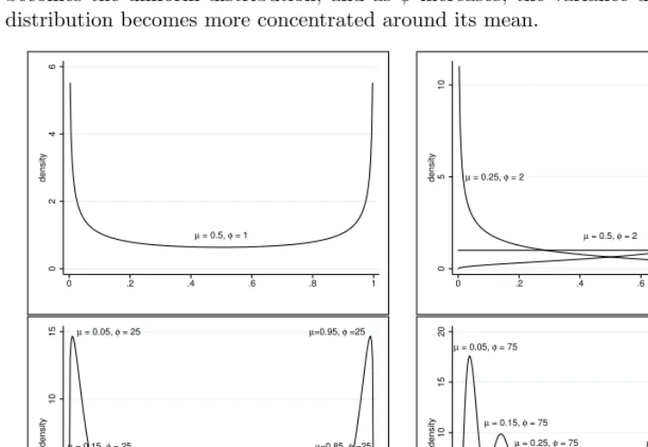
Beta distributions are convenient in modeling because they can display a variety of shapes depending on the values of their two parameters,µandφ. They are symmetric if

µ= (a+b)/2 and asymmetric for any other value ofµ. They can also be bell-, J-, and U-shaped. Figure 1 plots several beta probability densities for alternative combinations of µandφfor a variable defined in the (0,1) interval. At a value ofµ= 0.5 and small values of φ, the beta distribution is U-shaped; if µ= 0.5 and φ = 2, the distribution becomes the uniform distribution; and asφ increases, the variance decreases, and the distribution becomes more concentrated around its mean.

µ = 0.5, φ = 1

0

2

4

6

density

0 .2 .4 .6 .8 1

µ = 0.25, φ = 2

µ = 0.5, φ = 2

µ = 0.75, φ = 2

0

5

10

density

0 .2 .4 .6 .8 1

µ = 0.05, φ = 25

µ = 0.15, φ = 25

µ = 0.25, φ = 25

µ=0.5, φ =25 µ=0.75, φ =25

µ=0.85, φ =25

µ=0.95, φ =25

0

5

10

15

density

0 .2 .4 .6 .8 1

µ = 0.05, φ = 75

µ = 0.15, φ = 75

µ = 0.25, φ = 75

µ=0.5, φ =75

µ=0.75, φ =75

µ=0.85, φ =75

µ=0.95, φ =75

0 5 10 15 20 density

0 .2 .4 .6 .8 1

Figure 1. Probability density of the beta distribution for alternative combinations ofµ

andφ

Given a sample y1, y2, . . . , yn of independent random variables, each following the

probability density in (1), the beta regression model can be obtained by assuming that a functionv(·) of the mean of yi can be written as a linear combination of the set of

covariates in the vectorz_i,

v

_µ

i−a

b−a

=z′_iβ

µi(zi;β) =a+ (b−a)

exp (z′

iβ)

1 + exp (z′

iβ)

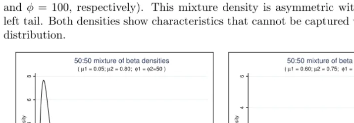
Pereira, Botter, and Sandoval (2012, 2013) present a more general beta regression model for variables defined at zero and in the interval [τ,1], which they named the “truncated inflated beta regression model”. It is a mixture model of a multinomial dis-tribution (with probability masses at 0,τ, and 1) and a beta distribution defined in the open interval (τ,1). In Gray, Hern´andez Alava, and Wailoo (Forthcoming), we extend the framework to the case where the second part can be a mixture of C-components of beta distributions incorporating the beta mixture described in Verkuilen and Smithson (2012). Mixtures of beta distributions can display a number of distributional shapes. Figure 2 shows two examples. The left panel plots a 50:50 mixture of two beta distri-butions, both with the same relatively high-precision parameter φ= 50 but with very different means,µ= 0.05 andµ= 0.80. This mixture displays the usual bimodal shape. The right panel also plots a 50:50 mixture, but the means of the 2 components are closer together (µ= 0.60 andµ = 0.75), and the precision parameters are different (φ = 10 and φ= 100, respectively). This mixture density is asymmetric with a bump on the left tail. Both densities show characteristics that cannot be captured with a single beta distribution. 0 2 4 6 8 density

0 .2 .4 .6 .8 1

( µ1 = 0.05; µ2 = 0.80; φ1 = φ2=50 )

50:50 mixture of beta densities

0

2

4

6

density

0 .2 .4 .6 .8 1

( µ1 = 0.60; µ2 = 0.75; φ1 = 10; φ2=100 )

50:50 mixture of beta densities

Figure 2. Mixture densities of beta distributions

Let us assume that the response variableyi is defined at the pointaand in the interval

[τ, b] witha < τ < b. The density ofyi conditional on three possibly different column

vectors of covariatesxi1,xi2, and xi3 can be written as

g(yi|xi1,xi2,xi3) =

            

P(yi=a|xi3) ifyi=a

P(yi=τ|xi3) ifyi=τ

P(yi=b|xi3) ifyi=b

"

1− P

s=a,τ,b

P(yi=s|xi3)

#

h(yi|xi1,xi2) ifyi∈(τ, b)

The probabilitiesP(yi|xi3) are derived from a multinomial logit model

P(yi=k|xi3) =

exp (x′_i3γ_k)

1 + P

s=a,τ,b

exp (x′

i3γs)

fork=a, τ, b (3)

wherex_i3is a column vector of variables that affect the probability of a boundary value of the response variable and γ_k is the vector of corresponding coefficients.

The probability density functionh(·) is a mixture of C-components of beta distri-butions with meansµci(zi;βc) and precision parametersφc, where c= 1, . . . , C,

h(yi|xi1,xi2) = C

X

c=1

[P(c|xi2)f{yi;µci(xi1;βc), φc, τ, b}] (4)

where f(·) is the beta density defined in (1). A multinomial logit model for the proba-bility of latent class membership is assumed to be

P(c|x_i2) = exp (x ′

i2δc)

PC

j=1exp (x′i2δj)

(5)

wherex_i2is a vector of variables that affect the probability of component membership,

δc is the vector of corresponding coefficients, and C is the number of classes used in the analysis. One set of coefficientsδc is normalized to zero for identification. In the intercept-only model, the probabilities of component membership are constant for all individuals.

Using (2), (3), (4), and (5), we can write the log likelihood of the sampley1, y2, . . . , yn

as

lnl(γ, β, δ, φ) = X

i:yi=a

lnP(yi=a|xi3,γ) + X

i:yi=τ

lnP(yi=τ|xi3,γ)

+ X

i:yi=b

lnP(yi=b|xi3,γ)

+ X

i:yi∈p

ln 





1− X

s=a,τ,b

P(yi=s|xi3,γ) 





+ X

i:yi∈(τ,b)

ln

C

X

c=1

[P(c|xi2)f{yi;µci(xi1;βc), φc, τ, b}]

!

wherei= 1, . . . , n.

in Stata usingbetaregor the community-contributed commandbetafit. In addition, the command betamixcan fit a finite mixture model using a beta distribution. If there are boundary values, betamixwarns the user and adds a small amount of noise (1e–6) to the boundary values after the response variable has been transformed to the interval [0,1] as in Basu and Manca (2012). This solution is not satisfactory when there are many observations at the boundary values. Provided there is theoretical justification, the user can request that betamixadd a second part to the model to add probability masses at any combination of the boundary points and the truncation value (if there is one).3

The description of the model above assumes constant precision parameters, but

betamix allows the precision parameters to depend on covariates using a log link such that

ln(φ) =x′_i4α

These models tend to be more difficult to fit and require good starting values. A good procedure to follow here is to start by fitting a model with constant precision as a stepping stone for the full model (Verkuilen and Smithson 2012).

We recommend that the reader become familiar with the idiosyncrasies of fitting mixture models (McLachlan and Peel 2000) before attempting to fit one. In particular, it is important to emphasize that mixture models are known to have multiple optima, and it is important to search for a global solution. Determining the number of compo-nents in a mixture is also not straightforward, and the analyst must exercise judgment in determining the appropriate number of components. Likelihood-ratio tests cannot be used to test models with different numbers of components, because it involves test-ing at the edge of the parameter space. The Bayesian information criterion (BIC) has been proposed as a useful indicator of the number of appropriate components, but other approaches also exist.

Exercise caution when using maximum likelihood estimation in small samples. Bias is usually not a problem in large samples, but in small samples, bias-corrected proce-dures are needed. It has been shown (Ospina, Cribari-Neto, and Vasconcellos 2006, 2011; Kosmidis and Firth 2010; Ospina and Ferrari 2012a) that for beta regressions, the biases of the regression parameters tend to be small, but larger biases are found for the precision parameter. In addition, the standard errors of the parameters are sys-tematically underestimated, leading to an exaggeration of the parameters’ significance. Ospina, Cribari-Neto, and Vasconcellos (2006) and Kosmidis and Firth (2010) use the same dataset (sample sizen= 32) to compare the effect of different adjustment proce-dures on the 12 estimated parameters and their standard errors. The present version of

betamixdoes not implement any bias-correction procedures for small samples.

3

Command syntax

3.1

betamix

Syntax

betamix depvar

if in weight , muvar(varlist) phivar(varlist)

ncomponents(#) probabilities(varlist) pmass(numlist) pmvar(varlist)

lbound(#) ubound(#) trun(trun) tbound(#) constraints(constraints)

vce(vcetype) level(#) maximize options search(spec) repeat(#)

Description

betamixis a community-contributed command that fits a generalized beta regression model using the truncated inflated beta model of Pereira, Botter, and Sandoval (2013) and the mixture beta regression model in Verkuilen and Smithson (2012).

Options

muvar(varlist)specifies a set of variables to be included in the mean of the beta regres-sion mixtures. The default is a constant mean.

phivar(varlist) specifies a set of variables to be included in the precision of the beta regression mixtures. The default is a constant precision parameter.

ncomponents(#)specifies the number of mixture components. #should be an integer. The default isncomponents(1).

probabilities(varlist) specifies a set of variables used to model the probability of component membership. The probabilities are specified using a multinomial logit parameterization. The default is constant probabilities.

pmass(numlist)specifies a list of exactly three number indicators (top inside bottom) showing the presence and position of the probability masses. For example,pmass(1 0 0)specifies a probability mass atb, the top limit of the dependent variable only;

pmass(0 0 0) specifies no probability masses (a beta mixture regression model);

pmass(1 0 1) specifies a model with probability masses at both limits of the de-pendent variable but no probability mass at the truncation point. The default is no probability masses at any point. Note thatpmass()requires a list of exactly three numbers, even if the model has no truncation.

lbound(#)specifies the user-supplied lower limit of the dependent variable. The default is lbound(0). Use this option if the dependent variable is limited in the interval (a, b). In this case, the upper bound of the interval also needs to be supplied using the option below.

ubound(#)specifies the user-supplied upper limit of the dependent variable. The de-fault isubound(1). Use this option if the dependent variable is limited in the interval (a, b). In this case, the lower bound of the interval also needs to be supplied using the option above.

trun(trun) determines whether there is truncation in the model and, if so, whether it is at the bottom or the top end. trun may benone, top, or bottom. Use none

if no truncation is required; usetop if the truncation (gap) is at the top [that is, the dependent variable is defined only in the interval (lbound(), tbound()) and the value ubound()]; use bottom if the truncation (gap) is at the bottom [that is, the dependent variable is defined only at the value lbound() and in the interval (tbound(), ubound())]. The default istrun(none).

tbound(#)specifies the user-supplied truncation value. If a truncation value is speci-fied, then the optiontrun()must be specified astoporbottom.

constraints(constraints); see [R]estimation options.

vce(vcetype) specifies how to estimate the variance–covariance matrix corresponding to the parameter estimates. vcetypemay beoim,opg,robust, orclusterclustvar. The default isvce(oim). The current version of betamixdoes not allowbootstrap

orjacknifeestimators; see [R]vce option.

level(#); see [R] estimation options.

maximize options: difficult,technique(algorithm spec),iterate(#),

no

log,

trace,gradient,showstep,hessian,showtolerance,tolerance(#),

ltolerance(#),gtolerance(#),nrtolerance(#),nonrtolerance,

from(init specs); see [R]maximize.

search(spec)specifies whether to useml’s initial search algorithm. specmay beonor

off. The default issearch(on).

repeat(#)specifies the number of random attempts to be made to find a better initial-value vector. This option is used in conjunction with search(on). The default is

repeat(100).

The likelihood functions of mixture models have multiple optima. The options

3.2

predict

Syntax

predict

type

newvar

if

in

, outcome(outcome)

predict {stub*|newvar1 ... newvarq}

if

in

, scores

Description

Stata’s standardpredictcommand can be used followingbetamixto obtain predicted values using the first syntax as well as the equation-level scores using the second syntax.

Options

outcome(outcome) specifies the predictions to be stored. There are two options for

outcome: y or all. The default is outcome(y), which stores only the dependent variable prediction in newvar. Use all to also obtain the predicted conditional means, precision parameters, and probabilities for each component in the mix-ture. These are stored asnewvar mu1,newvar mu2, . . . ,newvar phi1,newvar phi2, . . . and newvar p1, newvar p2, . . . , respectively. If an inflation model is specified,

all also stores the predicted probabilities of the multinomial logit part in new-varlb, newvarub, and newvar tb corresponding to the predicted probabilities of the lower bound, upper bound, and truncation bound. The probability of an ob-servation belonging to the beta mixture part of the model can be calculated as 1−newvarlb−newvar ub−newvar tb.

scorescalculates equation-level score variables.

4

The betamix command in practice

This section illustrates the use of the betamix command using a fictional dataset (betamix example data.dta) that can be downloaded when installing the command.

represent health states worse than death.4 _{Therefore,EQ-5D-3L is a limited dependent} variable with a lower limit equal to the value of the worst health state and an upper value of 1. In some cases, data on EQ-5D-3L have not been collected, and there is the need to predict what EQ-5D-3Lwould have been based on other available measures.

In this example, we are interested in estimating HRQoL measured byEQ-5D-3L5 as a function of a number of covariates. The data have 5,000 observations and is described below:

. use betamix_example_data . describe

Contains data from betamix_example_data.dta

obs: 5,000

vars: 5 23 May 2017 15:27

size: 90,000

storage display value

variable name type format label variable label

pain float %9.0g VAS pain scale [0,1]

haq_disability float %9.0g Health Assessment Questionnaire

eq5d_3l double %10.0g EQ-5D-3L utility

gender byte %8.0g gender_lbl

Gender (dummy variable)

age byte %8.0g Age in years

Sorted by: eq5d_3l

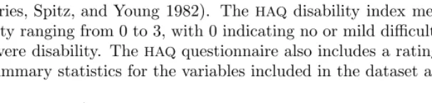
There are four additional variables in the dataset: the health assessment question-naire (HAQ) disability index, the pain score, age, and gender. The first two variables are collected in theHAQquestionnaire typically used in studies on rheumatoid arthritis (Fries, Spitz, and Young 1982). TheHAQdisability index measures physical function-ality ranging from 0 to 3, with 0 indicating no or mild difficulties and 3 indicating very severe disability. TheHAQquestionnaire also includes a rating scale for pain severity.6 Summary statistics for the variables included in the dataset are shown below.

. summarize

Variable Obs Mean Std. Dev. Min Max

pain 5,000 .0343357 .0239183 0 .1331617

haq_disabi~y 5,000 1.447728 .450958 0 3

eq5d_3l 5,000 .682108 .2246177 -.429 1

gender 5,000 .3954 .4889853 0 1

age 5,000 61.9178 11.00144 13 97

The average age in the dataset is 62 years, and 40% of the individuals are male. Figure 3 shows a histogram of the dependent variableEQ-5D-3L. The histogram presents a number of distributional characteristics that will need addressing when modeling.

4. For example, health states associated with extreme pain are often valued below zero in general population studies.

5. In this example, we use the UK valuation (Dolan et al. 1995).

EQ-5D-3L (UK valuation) is bounded between −0.594 and 1. Both of these values are possible. In the present dataset, there are no observations at the lower limit of −0.594. There is a pile of observations at the upper boundary of 1 (full health) and a gap between this mass at 1 and the previous value. This gap is not a sample issue, but a property of

EQ-5D-3L. There is a theoretical gap between 1 and the next feasible value. The size of the gap is country specific, and in theUKcase, there are no values between 1 and 0.883 creating a gap of 0.117. This gap is large relative to the total length of theEQ-5D-3L

interval (1.594). The distribution is also multimodal, and conditioning on variables is usually not enough to capture this aspect of the distribution. These idiosyncrasies have been previously reported (see, for example, Hern´andez Alava, Wailoo, and Ara [2012]).

0

1

2

3

4

5

Density

−.5 0 .5 1

EQ−5D−3L utility

Figure 3. Distribution ofEQ-5D-3L

The dataset will be used in two examples in sections 4.1 and 4.2: The first example will analyze the subsample of observations that are not in full health and show how to fit a mixture of beta regressions. The second example will use the full sample and, building on section 4.1, will show how to estimate an inflated truncated mixture of beta regressions.

4.1

Example 1: A mixture of beta regressions

For the purpose of this example and to show a simple version of the command, we ignore the observations at full health. In this subsample, the distribution ofEQ-5D-3L has a theoretical lower boundary of−0.594 and an upper boundary of 0.883 (highestEQ-5D-3L

value below full health). There are no observations at the lower boundary, but there are four observations at the upper boundary.7

We start by estimating a beta regression. Building on those results, we then estimate a mixture of beta regressions and compare the results.

We create local macros with the theoretical boundary values of the dependent vari-able as follows:

. local a = -0.594 . local b = 0.883

As a first step, we fit a beta regression model conditioning on age, gender, HAQ

disability index, and pain. This model can already be fit using thebetaregcommand by transforming the dependent variable and changing the observations at the boundaries by a small amount. Because there are only observations on the upper boundary, this model can be fit as follows:

. generate double eq5d_3l_t =(eq5d_3l-`a´)/(`b´-`a´) if eq5d_3l < 1 (539 missing values generated)

. replace eq5d_3l_t = eq5d_3l_t - 1e-6 if eq5d_3l_t==1 (4 real changes made)

. betareg eq5d_3l_t i.gender age haq_disability pain

(output omitted)

Usingbetamix, we can estimate the same beta regression as follows:

. betamix eq5d_3l if eq5d_3l < 1, muvar(i.gender age haq_disability pain) > lbound(`a´) ubound(`b´)

Warning. Some observations are on the upper boundary but no probability mass. A value of 1 is not supported by the beta distribution.

-1e-6 will be added to those observations.

initial: log likelihood = 3633.5637

(output omitted)

Iteration 5: log likelihood = 5507.4545

1 component Beta Mixture Model Number of obs = 4,461 Wald chi2(4) = 4854.70 Log likelihood = 5507.4545 Prob > chi2 = 0.0000

eq5d_3l Coef. Std. Err. z P>|z| [95% Conf. Interval]

C1_mu

gender

Male -.1906903 .0175407 -10.87 0.000 -.2250695 -.1563112 age .0007741 .0007811 0.99 0.322 -.0007568 .0023051 haq_disability -.9759785 .0247947 -39.36 0.000 -1.024575 -.9273818 pain -15.17255 .4339471 -34.96 0.000 -16.02307 -14.32203 _cons 3.826647 .0620419 61.68 0.000 3.705047 3.948247

C1_lnphi

_cons 2.974057 .021377 139.12 0.000 2.932158 3.015955

C1_phi 19.57115 .4183728 18.76809 20.40857

. matrix param = e(b) . estimates store beta1lc

All variables, with the exception of age, appear significant at conventional signifi-cance levels. Higher levels of disability (as measured byHAQdisability index) and pain are associated with lower levels of HRQoL (EQ-5D-3L), as expected. On average, males have lower levels ofEQ-5D-3L in this sample. The fitted model assumes a constant pre-cision parameterφ. Because a log link is used to ensure that the precision parameter is positive, the value of the untransformed parameter φ = 19.57 is also shown at the bottom of the output table.

Although the direction of the effect can be found directly from the estimates to find the magnitude of the effects and to interpret the estimates, it is helpful to use

margins. Here marginsis used following estimation to find the predictedEQ-5D-3L for

the estimation sample. The mean predictedEQ-5D-3Lis 0.6366, close to the mean in the estimation sample (0.6437).

. margins

Predictive margins Number of obs = 4,461

Model VCE : OIM

Expression : Prediction, predict()

Delta-method

Margin Std. Err. z P>|z| [95% Conf. Interval]

_cons .6366395 .0017476 364.29 0.000 .6332143 .6400648

. summarize eq5d_3l if e(sample)==1

Variable Obs Mean Std. Dev. Min Max

eq5d_3l 4,461 .6436987 .2070316 -.429 .883

In some cases, it is plausible that the variance of the distribution depends on ob-served covariates through their effect on the precision parameterφ. Models where the precision parameter is a function of covariates are more difficult to fit, and it is always recommended to start by fitting a model with constant variance and use it as a stepping stone.8

We now show how the commandbetamixcan be used to fit a more general model using mixtures of beta regressions. As always, when one fits mixture models, it is important that searches be carried out to ensure convergence to a global maximum (see section 2). The repeat()option can be used to increase the number of random attempts to find better starting values. Alternatively, if more control over the search strategy is required, the model can be optimized for a small number of iterations using a large number of different starting values. After this step, only the most promising trials (those with the highest likelihoods) are fully optimized, and the model with the highest likelihood is chosen.9

8. The accompanying do-file shows an example of how to specify and fit a model whereφis a function of a covariate.

We now fit a two-component beta regression mixture model. With the option

from(), we use the estimated parameters from the beta regression estimated earlier as initial parameter values to start the optimization.

. betamix eq5d_3l if eq5d_3l < 1, muvar(i.gender age haq_disability pain) > lbound(`a´) ubound(`b´) ncomponents(2) from(param)

Warning. Some observations are on the upper boundary but no probability mass. A value of 1 is not supported by the beta distribution.

-1e-6 will be added to those observations.

initial: log likelihood = 3953.8933

(output omitted)

Iteration 9: log likelihood = 6620.1281

2 component Beta Mixture Model Number of obs = 4,461 Wald chi2(8) = 6125.70 Log likelihood = 6620.1281 Prob > chi2 = 0.0000

eq5d_3l Coef. Std. Err. z P>|z| [95% Conf. Interval]

C1_mu

gender

Male -.1939933 .0140936 -13.76 0.000 -.2216163 -.1663703 age .0017032 .0006329 2.69 0.007 .0004628 .0029436 haq_disability -.8513914 .0195477 -43.55 0.000 -.8897041 -.8130786 pain -5.37046 .3753207 -14.31 0.000 -6.106075 -4.634845 _cons 3.463807 .0491347 70.50 0.000 3.367505 3.560109

C1_lnphi

_cons 4.399757 .0322272 136.52 0.000 4.336593 4.462922

C2_mu

gender

Male -.1192919 .0418525 -2.85 0.004 -.2013214 -.0372625 age -.0013071 .0018824 -0.69 0.487 -.0049965 .0023823 haq_disability -1.077175 .0588744 -18.30 0.000 -1.192567 -.9617834 pain -25.83155 .9151444 -28.23 0.000 -27.6252 -24.0379 _cons 4.215672 .1446903 29.14 0.000 3.932084 4.49926

C2_lnphi

_cons 2.657526 .0476911 55.72 0.000 2.564053 2.750999

Prob_C1

_cons .9734091 .0585439 16.63 0.000 .8586651 1.088153

C1_phi 81.43111 2.624296 76.44666 86.74056

C2_phi 14.26096 .6801207 12.98836 15.65826

pi1 .7257985 .0116511 .7023817 .7480338

pi2 .2742015 .0116511 .2519662 .2976183

. matrix param2=e(b) . estimates store beta2lc

The output now gives the parameter estimates for the two components of the model and for the multinomial logit10 _{that determines component membership. Note that in} this model, the probability of class membership is constant, but it can be allowed to

vary across individuals by including variables in the multinomial logit model using the

probabilities()option ofbetamix. Because the probability of belonging to each com-ponent is constant, the bottom of the output table shows these probabilities (pi1and

pi2) in an interpretable metric along with the precision parameters of both components (C1 phiandC2 phi).

In both components of the mixture, the HAQ disability index and pain score are negatively associated with average EQ-5D-3L, and being male is associated with lower

averageEQ-5D-3L, just as they were in the beta regression model. Age is significant in the

first component, where being older has a positive influence onEQ-5D-3L. Component 1 is

a dominant component with a probability (pi1) of 0.73. It is useful to use thepredict

command after estimation to visualize the two different components of the mixture.

. predict yhat2, outcome(all) . summarize yhat2* if e(sample)==1

Variable Obs Mean Std. Dev. Min Max

yhat2_mu1 4,461 .6954906 .0731658 .2635273 .8368744 yhat2_phi1 4,461 81.43111 0 81.43111 81.43111 yhat2_p1 4,461 .7257985 0 .7257985 .7257985 yhat2_mu2 4,461 .5599013 .2167423 -.3759323 .853509 yhat2_phi2 4,461 14.26096 0 14.26096 14.26096

yhat2_p2 4,461 .2742015 0 .2742015 .2742015 yhat2 4,461 .6583118 .1101933 .0881865 .8409589

In the estimation sample, the first component is estimated to have a meanEQ-5D-3L

of 0.6955 and a precision parameter φ = 81.43, whereas the second component has a slightly lower mean of 0.5599 and a more dispersed variance (φ = 14.26). Figure 4 plots the probability density of the mixture at this average together with each of the two individual components. The mixture probability density is more similar to the dominant component, but it has heavier tails.

0

5

10

y

0 .2 .4 .6 .8 1

Mixture Component 1 Component 2

As noted earlier, margins can be used to help interpret the model. For example,

marginsis used below to find the averageEQ-5D-3Lfor groups of patients with different levels of pain.

. margins, at(pain=(0(0.05)0.2))

Predictive margins Number of obs = 4,461

Model VCE : OIM

Expression : Prediction, predict()

1._at : pain = 0

2._at : pain = .05

3._at : pain = .1

4._at : pain = .15

5._at : pain = .2

Delta-method

Margin Std. Err. z P>|z| [95% Conf. Interval]

_at

1 .736477 .0021127 348.60 0.000 .7323362 .7406177 2 .641518 .0022414 286.22 0.000 .637125 .645911 3 .4912133 .0078346 62.70 0.000 .4758577 .5065689 4 .3413173 .0122964 27.76 0.000 .3172167 .3654178 5 .2366953 .0151763 15.60 0.000 .2069503 .2664404

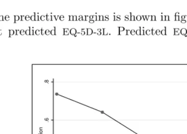
The plot of the predictive margins is shown in figure 5. Patients who report no pain have the highest predicted EQ-5D-3L. Predicted EQ-5D-3L decreases as reported pain increases.

.2

.4

.6

.8

Prediction

0 .05 .1 .15 .2

VAS pain scale [0,1]

Figure 5. Predictive margins with 95% confidence interval

. estimates stats _all

Akaike´s information criterion and Bayesian information criterion

Model Obs ll(null) ll(model) df AIC BIC

beta1lc 4,461 . 5507.454 6 -11002.91 -10964.49 beta2lc 4,461 . 6620.128 13 -13214.26 -13131.02

Note: N=Obs used in calculating BIC; see [R] BIC note.

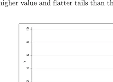
Figure 6 compares the probability densities of the mixture of two components and the beta regression model (calculated at the average). The mixture distribution has a larger peak at a higher value and flatter tails than the single component beta regression model.

0

2

4

6

8

10

y

0 .2 .4 .6 .8 1

Mixture Beta regression

Figure 6. Probability densities of the two-component beta mixture versus the beta regression

Models with a higher number of components should also be fit and compared to determine the best-fitting model.

4.2

Example 2: An inflated truncated mixture of beta regressions

In this example, we use the full dataset, which now includes the mass of values at the upper boundary of full health. Including these values creates a gap between the upper boundary and the previous feasible value (0.883) (see figure 3).11

We first fit an inflated truncated beta regression model. The new upper bound is now 1 (ub(1)), and the model includes a truncation at the top of the distribu-tion with no density between 0.883 and 1 (tb(0.883) trun(top)). The lower bound remains the same (lb(-0.594)). We allow the same variables to enter the beta re-gression (muvar(i.gender age haq disability pain)) and the inflation part of the model (pmvar(i.gender age haq disability pain)). There is inflation at the upper

bound but no inflation at the truncation point or at the lower bound (pmass(1 0 0)). In this example, it is not necessary to include an inflation at the truncation value be-cause there are only four observations with an EQ-5D-3L of 0.883. As in the previous example, there are no observations at the lower bound. The syntax to fit this model is reproduced below:

. betamix eq5d_3l, muvar(i.gender age haq_disability pain) lbound(-0.594) > ubound(1) tbound(0.883) pmass(1 0 0) pmvar(i.gender age haq_disability pain) > trun(top) from(param)

Note that this model is not the same as the Heckman selection model. It is equivalent to a two-part model, fit jointly under conditional independence between the two parts of the model. The output of this model is reproduced below:

Warning. Some observations are on the truncated boundary but no probability mass. A value of 1 is not supported by the beta distribution.

-1e-6 will be added to those observations.

Fitting full beta mixture model

initial: log likelihood = 2041.7186

(output omitted)

Iteration 5: log likelihood = 4507.4772

1 component Beta Mixture Model with inflation Number of obs = 5,000 Wald chi2(8) = 5477.05 Log likelihood = 4507.4772 Prob > chi2 = 0.0000

eq5d_3l Coef. Std. Err. z P>|z| [95% Conf. Interval]

C1_mu

gender

Male -.1906903 .0175407 -10.87 0.000 -.2250695 -.1563112 age .0007741 .0007811 0.99 0.322 -.0007568 .0023051 haq_disability -.9759784 .0247947 -39.36 0.000 -1.024575 -.9273818 pain -15.17255 .4339471 -34.96 0.000 -16.02307 -14.32203 _cons 3.826647 .0620419 61.68 0.000 3.705047 3.948247

C1_lnphi

_cons 2.974056 .021377 139.12 0.000 2.932158 3.015955

PM_ub

gender

Male -.4074599 .1191221 -3.42 0.001 -.6409349 -.1739848 age -.0006401 .0052235 -0.12 0.902 -.0108779 .0095978 haq_disability -2.729829 .1830281 -14.91 0.000 -3.088558 -2.371101 pain -81.13075 5.093264 -15.93 0.000 -91.11337 -71.14814 _cons 2.735824 .3788839 7.22 0.000 1.993225 3.478423

C1_phi 19.57115 .4183728 18.76809 20.40856

. estimates store infbeta1LC . matrix param2=e(b)

health. The likelihood of being in perfect health decreases as age, pain, and theHAQ

disability index increase. Note that, because this is a two-part model, the parameter estimates of the beta regression part of the model are the same as the parameters of the beta regression model fit in section 4.1.

Using the estimated parameters to initialize the algorithms, we also estimated the inflated truncated beta mixtures of two and three components. We also attempted to estimate a four-component mixture, but convergence was a problem. Results for the inflated truncated beta mixture of the three-component model are presented below:

. betamix eq5d_3l, muvar(i.gender age haq_disability pain) ncomponents(3) > lbound(-0.594) ubound(1) tbound(0.883) pmass(1 0 0)

> pmvar(i.gender age haq_disability pain) trun(top) repeat(500)

Warning. Some observations are on the truncated boundary but no probability mass. A value of 1 is not supported by the beta distribution.

-1e-6 will be added to those observations.

Fitting part 1: multinomial logit model Fitting full beta mixture model

initial: log likelihood = -977.04385

(output omitted)

Iteration 22: log likelihood = 5669.5447

eq5d_3l Coef. Std. Err. z P>|z| [95% Conf. Interval]

C1_mu

gender

Male -.1423077 .0506814 -2.81 0.005 -.2416414 -.0429739 age .0010803 .0021846 0.49 0.621 -.0032015 .0053621 haq_disability -1.108207 .0702167 -15.78 0.000 -1.245829 -.9705848 pain -28.63576 1.197209 -23.92 0.000 -30.98225 -26.28927 _cons 4.399697 .1652882 26.62 0.000 4.075738 4.723656

C1_lnphi

_cons 2.926432 .0667624 43.83 0.000 2.79558 3.057284

C2_mu

gender

Male -.1943955 .013987 -13.90 0.000 -.2218095 -.1669814 age .0015787 .0006276 2.52 0.012 .0003486 .0028088 haq_disability -.8512454 .0193374 -44.02 0.000 -.889146 -.8133448 pain -5.181831 .3752138 -13.81 0.000 -5.917236 -4.446425 _cons 3.455749 .0487475 70.89 0.000 3.360206 3.551292

C2_lnphi

_cons 4.366229 .0321085 135.98 0.000 4.303298 4.429161

C3_mu

gender

Male -.109573 .0435234 -2.52 0.012 -.1948773 -.0242687 age -.004191 .0019958 -2.10 0.036 -.0081028 -.0002792 haq_disability -.4509987 .0664523 -6.79 0.000 -.5812428 -.3207545 pain -5.012307 .879802 -5.70 0.000 -6.736687 -3.287927 _cons 1.332298 .1896052 7.03 0.000 .9606781 1.703917

C3_lnphi

_cons 4.978456 .1803428 27.61 0.000 4.624991 5.331922

Prob_C1

_cons 1.912517 .1730229 11.05 0.000 1.573398 2.251635

Prob_C2

_cons 3.115297 .1364868 22.82 0.000 2.847788 3.382806

PM_ub

gender

Male -.4074599 .1191221 -3.42 0.001 -.640935 -.1739848 age -.0006401 .0052235 -0.12 0.902 -.0108779 .0095978 haq_disability -2.72983 .1830281 -14.91 0.000 -3.088558 -2.371101 pain -81.13075 5.093264 -15.93 0.000 -91.11337 -71.14814 _cons 2.735824 .3788839 7.22 0.000 1.993226 3.478423

C1_phi 18.66093 1.245848 16.37212 21.2697

C2_phi 78.74615 2.52842 73.94325 83.86102

C3_phi 145.25 26.19479 102.0018 206.8351

pi1 .2233604 .0138256 .1974356 .251622

pi2 .7436474 .0125776 .7182305 .7675138

pi3 .0329922 .0045296 .0241143 .04187

Both the AIC and BIC are lowest for the three-component truncated inflated beta mixture model, suggesting it has the best model fit among the three models.

. estimates stats infbeta1LC infbeta2LC infbeta3LC

Akaike´s information criterion and Bayesian information criterion

Model Obs ll(null) ll(model) df AIC BIC

infbeta1LC 5,000 . 4507.477 11 -8992.954 -8921.265 infbeta2LC 5,000 . 5620.151 18 -11204.3 -11086.99 infbeta3LC 5,000 . 5669.545 25 -11289.09 -11126.16

Note: N=Obs used in calculating BIC; see [R] BIC note.

We again usepredictto help visualize the components:

. predict yhat3, outcome(all) . summarize yhat3*

Variable Obs Mean Std. Dev. Min Max

yhat3_mu1 5,000 .6141761 .2183959 -.3875231 .8636973 yhat3_phi1 5,000 18.66093 0 18.66093 18.66093 yhat3_p1 5,000 .2233604 0 .2233604 .2233604 yhat3_mu2 5,000 .7041177 .0750912 .2646665 .8360863 yhat3_phi2 5,000 78.74615 0 78.74615 78.74615

yhat3_p2 5,000 .7436474 0 .7436474 .7436474 yhat3_mu3 5,000 .2181699 .1072245 -.1579969 .4943131

yhat3_phi3 5,000 145.25 0 145.25 145.25

yhat3_p3 5,000 .0329922 0 .0329922 .0329922 yhat3_ub 5,000 .1078 .1867089 9.17e-07 .9079351

yhat3 5,000 .6919097 .1326988 .1050494 .9841948

In this sample, we see two components toward the top of the distribution with means 0.70 and 0.61 and a third component lower down in the distribution with mean 0.22. This third component has a much lower probability than the other two components (0.03) and appears to be capturing the mode at lower values ofEQ-5D-3L, seen in figure 3. Figure 7 plots the probability density of the three-component mixture and each of the components separately. It is clear in this case that this third component, although small, is important in modeling this dataset and helps handle the relatively small number of individuals withEQ-5D-3Lvalues close to the value of death.

5

Concluding remarks

distribu-0

5

10

y

0 .2 .4 .6 .8 1

Mixture Component 1 Component 2 Component 3

Figure 7. Probability densities of the three-component truncated inflated beta mixture model each individual component (for values below full health)

tion and can model positive probabilities at the boundaries and the truncation value. There is no need to manually transform variables bounded in the interval (a, b) to the (0,1) interval, because the command will take care of the transformation.

It is important to start fitting less complex models and slowly build them up; oth-erwise, convergence problems are likely. The likelihood functions of mixture models are known to have multiple optima. It is important to thoroughly search around the parameter space to avoid local solutions.

6

Acknowledgments

We thank the editor and an anonymous referee for very helpful comments and sugges-tions. M´onica Hern´andez Alava acknowledges support by the Medical Research Council under grant MR/L022575/1. The views expressed in this article, as well as any errors or omissions, are only of the authors.

7

References

Basu, A., and A. Manca. 2012. Regression estimators for generic health-related quality of life and quality-adjusted life years. Medical Decision Making 32: 56–69.

Berggren, N., S.-O. Daunfeldt, and J. Hellstr¨øm. 2014. Social trust and central-bank independence. European Journal of Political Economy 34: 425–439.

Buis, M. L. 2010. zoib: Stata module to fit a zero-one inflated beta distribution by maximum likelihood. Statistical Software Components S457156, Department of Eco-nomics, Boston College. https: // ideas.repec.org / c / boc / bocode / s457156.html.

De-partment of Economics, Boston College. https: // ideas.repec.org / c / boc / bocode / s435303.html.

Cook, D. O., R. Kieschnick, and B. D. McCullough. 2008. Regression analysis of pro-portions in finance with self selection. Journal of Empirical Finance 15: 860–867.

De Paola, M., V. Scoppa, and R. Lombardo. 2010. Can gender quotas break down negative stereotypes? Evidence from changes in electoral rules. Journal of Public Economics 94: 344–353.

Dolan, P., C. Gudex, P. Kind, and A. Williams. 1995. A social tariff for EuroQol: Results from aUK general population survey. Discussion Paper No. 138, University of York, Centre for Health Economics. http: // www.york.ac.uk / che / pdf / DP138.pdf.

EuroQol Group. 1990. EuroQol—A new facility for the measurement of health-related quality of life. Health Policy 16: 199–208.

Ferrari, S., and F. Cribari-Neto. 2004. Beta regression for modelling rates and propor-tions. Journal of Applied Statistics 31: 799–815.

Fries, J. F., P. W. Spitz, and D. Y. Young. 1982. The dimensions of health outcomes: The health assessment questionnaire, disability and pain scales. Journal of Rheuma-tology 9: 789–793.

Gray, L. A., M. Hern´andez Alava, and A. J. Wailoo. Forthcoming. Development of methods for the mapping of utilities using mixture models: Mapping the AQLQ-Sto

EQ-5D-5L andHUI3in patients with asthma. Value in Health.

Hern´andez Alava, M., and A. Wailoo. 2015. Fitting adjusted limited dependent variable mixture models toEQ-5D. Stata Journal15: 737–750.

Hern´andez Alava, M., A. J. Wailoo, and R. Ara. 2012. Tails from the peak district: Adjusted limited dependent variable mixture models of EQ-5D questionnaire health state utility values. Value in Health15: 550–561.

Ji, Y., C. Wu, P. Liu, J. Wang, and K. R. Coombes. 2005. Applications of beta-mixture models in bioinformatics. Bioinformatics21: 2118–2122.

Johnson, N. L., S. Kotz, and N. Balakrishnan. 1995. Continuous Univariate Distribu-tions, vol. 2. 2nd ed. New York: Wiley.

Kent, S., A. Gray, I. Schlackow, C. Jenkinson, and E. McIntosh. 2015. Mapping from the Parkinson’s disease questionnaire PDQ-39 to the generic EuroQol EQ-5D-3L. Medical Decision Making 35: 902–911.

Kieschnick, R., and B. D. McCullough. 2003. Regression analysis of variates observed on (0, 1): Percentages, proportions and fractions. Statistical Modelling 3: 193–213.

McLachlan, G., and D. Peel. 2000. Finite Mixture Models. New York: Wiley.

Ospina, R., F. Cribari-Neto, and K. L. P. Vasconcellos. 2006. Improved point and interval estimation for a beta regression model. Computational Statistics and Data Analysis 51: 960–981.

. 2011. Erratum to “Improved point and interval estimation for a beta regression model” [Comput. Statist. Data Anal. 51 (2006) 960–981]. Computational Statistics and Data Analysis 55: 2445.

Ospina, R., and S. L. P. Ferrari. 2010. Inflated beta distributions. Statistical Papers

51: 111–126.

. 2012a. On bias correction in a class of inflated beta regression models. Inter-national Journal of Statistics and Probability 1: 269–282.

. 2012b. A general class of zero-or-one inflated beta regression models. Compu-tational Statistics and Data Analysis 56: 1609–1623.

Paolino, P. 2001. Maximum likelihood estimation of models with beta-distributed de-pendent variables. Political Analysis 9: 325–346.

Papke, L. E., and J. M. Wooldridge. 1996. Econometric methods for fractional response variables with an application to 401(K) plan participation rates. Journal of Applied Econometrics 11: 619–632.

. 2008. Panel data methods for fractional response variables with an application to test pass rates. Journal of Econometrics145: 121–133.

Pereira, G. H. A., D. A. Botter, and M. C. Sandoval. 2012. The truncated inflated beta distribution. Communications in Statistics—Theory and Methods41: 907–919.

. 2013. A regression model for special proportions. Statistical Modelling 13: 125–151.

Smithson, M., and J. Verkuilen. 2006. A better lemon squeezer? Maximum-likelihood regression with beta-distributed dependent variables. Psychological Methods 11: 54– 71.

Verkuilen, J., and M. Smithson. 2012. Mixed and mixture regression models for con-tinuous bounded responses using the beta distribution. Journal of Educational and Behavioral Statistics 37: 82–113.

About the authors

Laura A. Gray is a research associate in health econometrics in the Health Economics and Decision Science section in ScHARR, University of Sheffield,UK. Her main research interest is microeconometrics, particularly in relation to health behaviors and obesity.