The evolution of host defence to parasitism in fluctuating environments

This is a repository copy of The evolution of host defence to parasitism in fluctuating environments.

White Rose Research Online URL for this paper: http://eprints.whiterose.ac.uk/124875/

Version: Supplemental Material

Article:

Ferris, C. and Best, A. (2018) The evolution of host defence to parasitism in fluctuating environments. Journal of Theoretical Biology, 440. pp. 58-65. ISSN 0022-5193

https://doi.org/10.1016/j.jtbi.2017.12.006

Article available under the terms of the CC-BY-NC-ND licence (https://creativecommons.org/licenses/by-nc-nd/4.0/).

eprints@whiterose.ac.uk https://eprints.whiterose.ac.uk/

Reuse

This article is distributed under the terms of the Creative Commons Attribution-NonCommercial-NoDerivs (CC BY-NC-ND) licence. This licence only allows you to download this work and share it with others as long as you credit the authors, but you can’t change the article in any way or use it commercially. More

information and the full terms of the licence here: https://creativecommons.org/licenses/

Takedown

If you consider content in White Rose Research Online to be in breach of UK law, please notify us by

A

Trade-Off Function

a

(

β

)

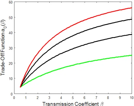
Figure A.1 shows how the trade-off function defined by equation (4) in the main text varies with

transmission coefficientβ for different values of c.

Figure A.1: Trade-off functiona0(β) as defined in equation (4) of the main text for varying

transmis-sion coefficientβ and different values of cincreasing from 1.5 (green) to 3 (red) in steps with size 0.5. Default parameters were otherwise used.

B

How To Find The Host Fitness When

γ >

0

The adaptive dynamics method involves adding a rare mutant with susceptible and infected population

sizes Sm, Im and transmission coefficient βm very close to the resident transmission coefficient β.

Assumptions for this method are outlined in the main text. We therefore have equations for the

mutant population:

dSm

dt =a0(βm)(1 +δsin(2πt/ǫ))(1−q(N +Nm))Sm−bSm−βmSm(I+Im) +γIm, (B.1)

dIm

dt =βmSm(I+Im)−(b+α+γ)Im, (B.2)

whereNm =Sm+Im is the total mutant population, andS =S(t),I =I(t) are the resident dynamics

Equations (B.1) and (B.2) are easily linearised using the assumption that the mutant is initially

rare. To analyse how the host evolves, we consider the mutant’s fitness, defined to be the long-term

exponential growth rate of the mutant in the current environment (Metz et al., 1992). Forγ >0, the

mutant’s fitness is the largest Lyapunov exponent.

To find the Lyapunov exponent, suppose that we have a fundamental solutionX(t) = (Sm(t)Im(t))

of the linearised mutant equations (B.1), (B.2) (Grimshaw, 1990). We can then rewrite the problem

as:

dX(t)

dt =A(t)X(t) (B.3)

where A(t) is a 2 x 2 matrix containing the periodic coefficients. The solution X(t) is unlikely to be

periodic, but we can write the linearly independent solutions to (B.3) in the form Xi(t) = eµitpi(t)

for i∈ {1,2}, where the pi are periodic with period T. From Grimshaw (1990), we can write:

X(t+T) =X(t)C ∀ t ≥0, (B.4)

whereCis a non-singular constant 2 x 2 matrix. We now know that the mutant population grows or

decays depending on the signs of the µi, which are related to the eigenvalues ofC byρi =eµiT. The

mutant fitness is therefore the largest of the µi: if they are both negative, the mutant dies out; if at

least one is positive, the mutant grows.

We are predominantly interested in the sign of the fitness, i.e. whether or not max{µ1, µ2}is greater

or less than zero. This is equivalent to considering whether or not the maximum of the eigenvalues

ρi is greater or less than 1. Therefore the fitness for our seasonal system is the largest eigenvalue of

Cminus 1.

We cannot find the eigenvalues of C analytically because we cannot solve the mutant equations

analytically (Klausmeier, 2008). However, we can find C numerically by setting t = 0 in (B.4),

then choosing two linearly independent initial conditions X(0). By running the mutant equations

within the current resident dynamics, this then gives us four equations for the elements of C in the

numerically found components of X(T). The simplest initial conditions to implement are (1 0) and

acquired C.

Note that sinceCis a non-negative matrix, the Perron-Frobenius theorem applies and the largest

eigenvalueρofCis non-negative. For some positive integerk, we can sett=t′_{+ (k−1)T in equation}

(B.4) to obtain:

X(t′ _{+kT) =X(t}′_)Ck _{∀ t}′ _{≥0. (B.5)}

By setting t′ _{= 0, we can find the elements of C}k _{numerically by running the mutant dynamics up}

to time kT. From linear algebra results, we know that the eigenvalues of Ck are ρk

i. The fitnesses

(ρ−1) and (ρk_{−1) obtained from equations (B.4) and (B.5) respectively are of the same sign when}

ρ is non-negative, hence we find the correct sign for the fitness when the mutant dynamics are run

up to time kT for some positive integer k.

C

Method for Finding the Population Averages

Let T be the period of oscillation of the hosts (note that this is some integer multiple of ǫ), so we

haveS(t+T) =S(t) etc. We can take the average of dS_dt(t) and dI_dt(t) over this period to find:

1 T

Z P1

P0

dS

dtdt= [S(t)]

P1

P0 = 0, (C.1)

and

1 T

Z P1

P0

dI

dtdt= [I(t)]

P1

P0 = 0, (C.2)

where P1 = P0 +T for some arbitrary time P0 > 0 after the population has reached a dynamic

attractor. We also have:

1 T

Z P1

P0

1 S

dS

dtdt = [ln(S(t))]

P1

P0 = 0. (C.3)

and

1 T

Z P1

P0

1 I

dI

dtdt= [ln(I(t))]

P1

By using equation (C.4) and the model equation for dI_dt(t), we find with some rearranging that:

ˆ S = 1

T

Z P1

P0

S(t)dt= α+b+γ

β . (C.5)

Using equation (C.2) and the model equation for dI_dt(t), we find that:

ˆ

I = β (α+b+γ)

1 T

Z P1

P0

S(t)I(t)dt . (C.6)

From equations (C.1) and (C.6), we can find an alternative form for ˆI:

ˆ

I = 1 (α+b)

1 T

Z P1

P0

{a(t)S(t)(1−qN(t))}dt−bSˆ

. (C.7)

D

Simulation Example

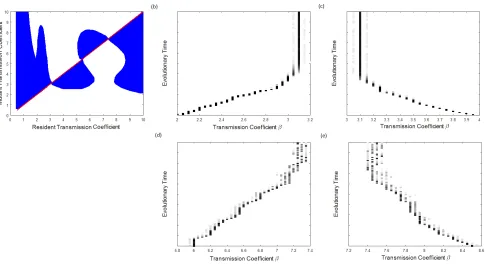
Throughout this paper we confirmed the evolutionary behaviour near the singular points found using

PIPs and simulations. Figure D.1 shows an example of a bistability case similar to that examined in

the main text. The PIP shows that three singular points exist, specifically 2 CSSs (β∗

L = 3.0941 &

β∗

H = 7.3764) separated by a repeller (βR∗ = 5.3511). Simulations confirm the types seen in the PIP,

with the host evolving towards β∗

L for initial transmission coefficient β0 < βR∗ (figures (b) & (c)) and

towardsβ∗

H for β0 > βR∗ (figures (d) & (e)). This example also demonstrates that the approximation

method used to find the fitness is somewhat robust, since in the simulations we have relaxed the

assumptions that the resident is monomorphic and that mutations are very small.

E

Stability of Solutions for

γ

= 0

In figure 1(c) in the main text, we claimed that the discrete change in singular point β∗ _{is due to a}

change in attractor in the population dynamics. Figure E.1 shows the stability of the 1- and 2-year

solutions. We found that for varying amplitude δ, the 1-year solution (black) remains stable up to

Figure D.1: (a) Pairwise-invasion plot, where blue indicates positive mutant fitness, and the red line is β =βm. (b),(c),(d),(e) Simulations of the evolutionary behaviour for initial resident transmission

coefficient (b) β0 = 2, (c) β0 = 4, (d) β0 = 6 & (e) β0 = 8.5. Darker squares indicate a higher

proportion of the population with the corresponding transmission coefficient β. Parameters were set at default values except ˆa0 = 104, γ = 0.03 & δ= 0.75.

unstable). The red curve that emerges is the 2-year solution. This is stable for a very short time but

then has a fold and goes back until about δ = 0.57 where another fold produces the stable 2-year

solution that continues up to δ = 1. The two solutions give different singular points, and bistability

between the 1- and 2-year solutions causes an overlap for δ ∈ (0.57,0.63) between each branch of

singular points, as seen in figure 1(c) from the main text.

Both singular points were found to be CSSs, although for amplitudes within the bistability region,

the T = 2 singular point can only be reached by evolution from initial transmission coefficient β0

greater than the lower bound of the bistability region. This is due to the fact that for β0 less than

this point, the population never reaches the period-doubling bifurcation, see figure E.1(b), and so it

doesn’t switch between the attractors, and hence the host evolves towards the lower singular point

Figure E.1: (a) Stability of solutions to the population equations (1) & (2) in the main text when amplitudeδ varies. Black lines - solution with period 1; Red lines - solution with period 2; Solid lines - stable solution; Dashed lines - unstable solution. (b) 2D bifurcation plot of transmission coefficient βvs amplitudeδ. Red - period-doubling bifurcation; Blue - fold bifurcations. Both graphs use default parameters with ˆa0 = 104, γ = 0 &β = 2.87 in (a), and were created using AUTO-07p.

F

Evolution of hosts with a longer lifespan

Figure F.1: Two-dimensional contour plots showing the change in the singular pointβ∗ _{as amplitude} δand (a) recovery rateγ, (b) crowding factor qand (c) virulenceα vary. Other parameters were fixed at default values from the main text with γ = 1 & b= 0.5.

In this section we let the parameters take default values with baseline mortality rate decreased to

b= 0.5 (longer-lived hosts). Figure F.1 shows the CSS singular pointβ∗ _{for varying amplitudeδwith}

recovery rate γ, crowding factor q and virulence α. In this case, the evolutionary behaviour of the

host remains the same for all values of δ and is caused by changes in the average infected population

in all three cases. These results are in contrast to those in the main text, where we found that the

evolutionary behaviour changes for high amplitudes. Note in particular that the host evolves highest

the dip is smaller for low amplitudes and so doesn’t show up in figure F.1(c). This indicates that the

evolution of hosts with a shorter lifespan may be more complicated for high amplitude birth rates, &

that high amplitudes has a more significant impact on the populations dynamics for shorter lifespans.

However, we can expect the same behaviour for high or low amplitude birth rates for longer-lived

hosts.

Literature Cited Only in the Appendix

E. Doedel and B. Oldman. AUTO 07-p: Continuation and bifurcation software for ordinary differential