Real time computation of Haar like features at generic angles for detection algorithms

(1)

Real-time Computation of Haar-like features at

generic angles for detection algorithms

A. L. C. Barczak, M. J. Johnson & C. H. Messom

Institute of Information & Mathematical Sciences Massey University at Albany, Auckland, New Zealand.

This paper proposes a new approach to detect rotated objects at distinct angles using the Viola-Jones detector. The use of additional Integral Images makes an approximation the Haar-like features for any given angle. The proposed approach uses different types of Haar-like features, including features that compute areas at 45o

, 26.5o

and 63.5o

of rotation. Given a trained classifier (using normal features) a conversion is made using a pair of features so an equivalent value is computed for any angle. This conversion is only an approximation, but the errors are constrained and they would have limited impact on the final accuracy of the classifier. We discuss the sources of errors in the computation of the Haar-like features and show through experiments that in natural images the errors are often negligible.

Keywords: Pattern Recognition, Rotation Invariant Detectors, Real-time Object

Detec-tion, Haar-like Features, Viola-Jones Detector.

1 Introduction

The Viola-Jones detector (1)(2) has received considerable attention since its publication. It has been used mainly for face detection (3), face recognition (4) and hands detection (5). Other uses include robot-soccer ball detection(6) and ecological applications such as wild life surveillance(7). Due to the non-invariant nature of the Haar-like features, classifiers trained with this method are often incapable of finding rotated objects. It is possible to use rotated positive examples during training, but such a monolithic approach often results in inaccurate classifiers (8). Besides such a classifier would not inform at which angle the object was found. Alternatively one can train a set of classifiers, each one specialised in a certain angle interval. Although this might achieve the detection accuracy required, it also makes the training computationally much more expensive. Ideally one should be able to train a classifier once and detect the object at a generic angles.

The Viola-Jones detector compute Haar-like features using Integral Images, a special data structure that speeds-up the calculation. In practise it is only possible to compute Haar-like features accurately at a fixed angle. The angle is determined by the way the Integral Image is created. Currently two types of Integral Images are in use, one capable of computing areas at 0o

and another at 45o_{. If the feature type is converted it is also possible to compute features at other}

quadrants (90o_{, -90}o_{and 180}o_{from the original) using the same Integral Image (8). Therefore one}

can compute features at eight different angles using two Integral Images.

The solution proposed by this paper makes use of two additional Integral Images that computes angles at 26.5o_{and 63.5}o_{to approximate the Haar-like feature values at a generic angle. We show}

(2)

type 7 1/2 1/2 type 3 1/3 1/3 1/3 type 6

1/3 1/3 1/3

type 2

1/3 1/3 1/3

type 5 1/2 1/4 1/4 1/2 1/2 type 1 type 4

1/4 1/2 1/4

type 0 1/2 1/2 1/3 1/4 1/2 1/4 1/2 1/4 1/4 1/3 1/3 1/2 1/2 1/3 1/3 1/3 1/3 1/3 1/3 1/2 1/2 1/2 1/2 type 14 type 10 type 11

type 15 type 16 type 12 type 13

type 17 1/2 1/2 1/2 1/2 1/3 1/3 1/3 1/3 1/3 1/3 1/4 1/2 1/4 1/4 1/4 1/2 1/3 1/3 1/3 1/2 1/2

o Normal Features (0 )

Rotated Features (45 )o

[image:2.612.243.381.57.306.2]

o Rotated Features (26.5 )

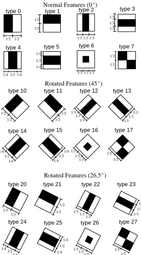
Figure 1: Classifiers using the Normal features can be converted to the other types.

The paper is organised as follows: a brief description of the Viola-Jones methods and algorithms are presented (training and detection), including some important extensions added by other au-thors. Next the proposed method for detection with rotation is explained. The following section presents experiments regarding error analysis. Finally the conclusions point out the limitations and possible improvements on a generic rotation invariant detector using Haar-like features.

2 Viola-Jones Detector

The Viola-Jones detector has three main characteristics: it uses an over-complete set of Haar-like features, it uses Integral Images to compute areas (sum of pixels) in a very efficient way and it uses Adaboost for training.

Haar-like features can be constructed in many shapes and computed in different ways. Figure 1 shows three groups of Haar-like features. The original implementation (1) only used types 0,1,2,3 and 7. The implementation in OpenCV (9) used all types but types 7 and 17. The third group was implemented for the error analysis presented in this paper. The details of the Integral Image concept can be found in (1).

Viola and Jones used a customised version of Adaboost, which was first created by Freund and Schapire (10) to solve machine learning problems. One of the changes made to the algorithm was the creation of many layers. Each layer is trained by several rounds of Adaboost. To improve training speed as well as detection performance they introduced some heuristics.

(3)

o

45 (twisted) 26.5 o

height

width

height

t_height t_width

normal

t_width t_height/2

[image:3.612.186.439.59.182.2]

width

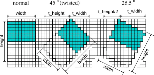
Figure 2: An approximated equivalence between a normal and a 26.5o _{Haar-like feature.}

the introduction of a fast heuristic to find a sub-optimal feature by McCane and Novins (13). They reported an improvement in the training time with just minor effects on the detection phase.

2.1 Error sources in the computation of Haar-like features

In practise when computing the Haar-like features in digital images one cannot expect an exact value. Although the features are a simple comparison between areas (sum of pixels), there are three main sources of errors:

• the rounding up of the feature sizes due to scale changes

• the rounding up of the position of the feature in relation to a fixed point in the image

• the approximation due to some pre-processing of the image (rotation, scaling etc).

The first error source can be partially compensated by a correction factor that ensures that the areas are proportional to the theoretical definition of that particular feature. Lienhart et al. (11) suggested a correction to this problem. A correction factor is computed so that the weights of the different rectangles of a feature keep the original area ratio between them. One experiment that should be done when testing any implementation is to find the value of the features in a grayish image with equal pixel values all over the image. All features at any size and scale should yield zero.

In our implementation we used aunit Integral Image that counts the number of pixels in each area that composes a Haar-like feature. Although this requires extra look-ups it allows to rapidly compute the correction factors. One advantage of this approach is that the unit Integral Image does not change when new frames are being assessed, saving precious time. The unit Integral Image is only necessary for the the rotated features (45o_{, 26.5}o _{and 63.5}o_{) mainly because for the}

normal (0o_{) case the number of pixels can be based on the width and height of the feature.}

The second error source cannot be compensated without a more complicated approach such as computing sub-pixel values for the areas. This is not usually a good approach because it loses the advantage of computing areas very rapidly with the assistance of the Integral Images.

The third error occurs when comparing the same image with its counterpart after a processing operation such as scaling and rotation. Anti-aliasing techniques applied when scaling images can cause variations even if the features can fit the position and the sizes perfectly. Although this error is not directly related to the features’ definition or implementation itself, it is an important source of errors during the detection phase or testing.

2.2 Computing Haar-like features at 45

o

and 26.5

o

(4)

I

₃

I

₁

I

2 CASE 2 (odd,odd) CASE 4 (odd,even)

I

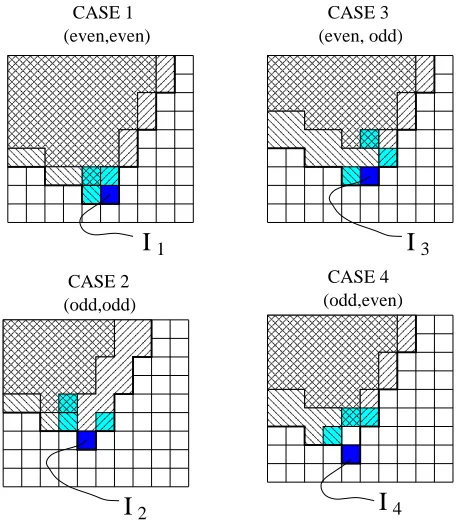
4 (even,even) CASE 1 (even, odd) CASE 3 !!!!!!!! !!!!!!!! !!!!!!!! !!!!!!!! !!!!!!!! !!!!!!!! """""""" """""""" """""""" """""""" """""""" """""""" ### ### $$ $$ %%%%%%%%% %%%%%%%%% %%%%%%%%% %%%%%%%%% %%%%%%%%% %%%%%%%%% %%%%%%%%% %%%%%%%%% &&&&&&&&& &&&&&&&&& &&&&&&&&& &&&&&&&&& &&&&&&&&& &&&&&&&&& &&&&&&&&& &&&&&&&&& '''''' '''''' '''''' '''''' (((((( (((((( (((((( (((((( ))))) ))))) ))))) ))))) ))))) ))))) ))))) ))))) **** **** **** **** **** **** **** **** ++ ++ ,, ,, ---.. .. /// /// 00 00

Figure 3: Computing the Integral Image for 26.56o _recursively

[image:4.612.199.428.56.317.2]

and the twisted features are not mathematically equivalent in digital processing due to the fact that the twisted Integral Image needs slightly distorted rectangles to correctly compute an area. Figure 2 shows an example were two features, one normal and the other twisted, would compute similar areas. Notice the double pixel on two vertexes of the twisted feature. This is necessary in order to get the correct alignment so the Integral Image can supply the correct sum of pixels (9). Yet another approximation has to be made when computing the width and the height of the twisted feature, as this calculation often yields a sub-pixel value.

Unfortunately for other angles the solution is not trivial, as the shapes of the areas covered by one element of the Integral Image changes depending on the parity of the coordinates. However, there is a partial solution for the case where the ratio is 1:2 or 2:1. As these angles also allow the computation on the other quadrants, four Integral Images will suffice to divide 360o_{in 16 regions}

(only approximately symmetric).

Next we formalise the calculation of the Integral Image for the case of 26.5o_{. The other case}

(63.5o_{) is analogous. Each element of the Integral Image will cover different areas of the}

im-age. There are four cases that depend on the parity of the coordinates ( (even,even), (even,odd), (odd,even) and (odd,odd) coordinates). Figure 3 shows the four cases and the areas that they cover respectively. The Integral Image can be computed recursively using the following equations:

I1(x,y)=I(x₋1,y)+I(x,y₋1)−I(x₋1,y₋1)+im(x,y) (2.1)

I2(x,y)=I(x+1,y₋1)+I(x₋1,y₋1)−I(x₋1,y₋2)+im(x,y) (2.2)

I3(x,y)=I(x₋1,y)+I(x+1,y₋1)−I(x,y₋2)+im(x,y) (2.3)

I4(x,y)=I(x−1,y−1)+I(x+1,y−2)−I(x,y−2)+im(x,y)+im(x,y−1) (2.4)

(5)

The computation of the Haar-like features at 26.5o _{also demands that the alignment of the 4}

points are coherent with the creation of the Integral Image. Extra operations to analyse the parity of the coordinates are necessary. The possible combination of the parities of 4 points mount to 64 cases. Most cases do not need any correction. About a dozen cases need a displacement of one position on one or two points so the alignment is respected.

2.3 Converting features to generic angles

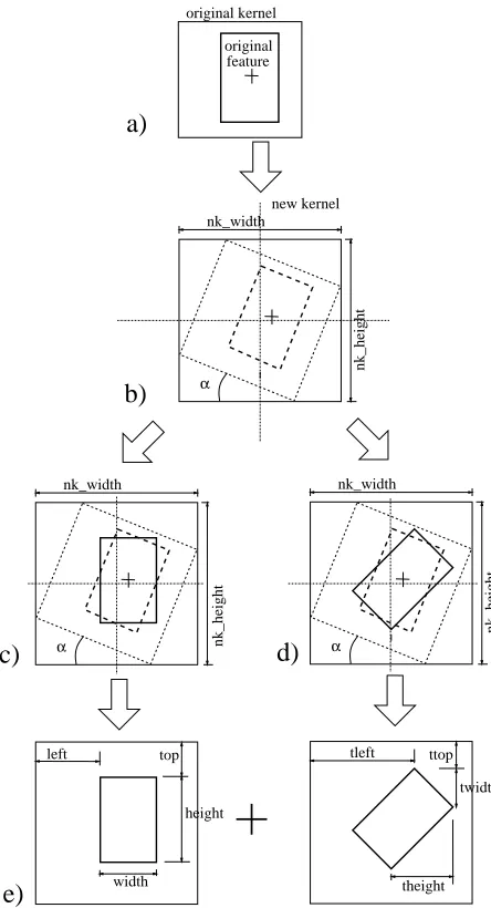
We propose using a function of the values of two features to approximate the value for a feature rotated at a generic angle. We call this approachpair of equivalent features(PEF).This is achieved using a weighted sum of the two equivalent features and a conversion of feature positions, feature sizes and feature types. Figure 4 shows how this conversion is done for the case where normal and 45o_{features are used. For an angle}_α_{the new features has to be positioned on a new kernel, larger}

in size to accommodate the rotation of the second feature. For example, for angles between 0o_and

45o_{formula 2.5 applies. For angles larger than 45}o _{there is also a feature type change to be made.}

For example, the PEF of a type 0 feature for angles between 0o_{and 45}o_{will be a normal feature}

of type 0 and a twisted feature of type 10. If the angle is between 45o _{and 90}o_{, the PEF will be}

a normal feature of type 1 and a twisted feature of type 10 (figure 5). For other angles the PEF may be computed from other pairs, in some cases involving a change of sign.

The value of the PEF can be approximate by the following equation:

V =Vnormal.(45o−α)/45o+Vtwisted.α/45o (2.5)

Where: Vnormalis the Value for the normal feature,Vtwistedis the value for the twisted feature

and V is the weighted average that depends on the angleα(between 0o_{and 45}o_).

Analogous to the case where the PEF is computed with a normal and a 45o _{angle, one can}

approximate the feature value for any angle between 0o_{and 26}_.₅o_:

V =Vnormal.(26.5o−α)/26.5o+V26.α/26.5o (2.6)

Where: Vnormal is the Value for the normal feature, V26 is the value for the feature at 26.5o and V is the weighted average that depends on the angleα(between 0o_{and 26.5}o_).

2.4 PEF errors

A Haar-like feature value will depend on the distribution of the pixels in the area where it is applied. The maximum value for many types of Haar-like features occurs when an edge is located in the middle of the feature. In order to maximise the absolute value of the feature it is also necessary that all the values of the pixels on one side of the edge are zeros and all the other pixel values are maximum (for example, 255 in a grey scale image).

From this point lets call the maximum value of a feature at a generic scale to be MAX, so that any feature value can vary from -MAX to MAX. Lets suppose that we could compute a

type 0 Haar-like feature at an angle of 22.5o _{over an edge presented by the image. We assume}

(6)

left top

width

height nk_width

α nk_height

nk_width

nk_height

α

tleft ttop

twidth

theight

c)

d)

e)

original kernel

feature original

nk_width new kernel

nk_height

α

b)

a)

[image:6.612.200.422.134.544.2]

(7)

type 0

features Normal

features Twisted ranges

Angle

=

type 11 −135 ∼ −90

−90 ~ −45

−45 ~ 0

0 ~ 45

45 ~ 90

90 ~ 135

=

+

type 1 − type 10

type 1

type 0 _{type 11}

type 0 type 10

− type 1 type 10

[image:7.612.199.420.69.318.2]

− type 1 _{−type 11}

Figure 5: An example of PEFs for a type 0 feature considering a number of angle ranges.

b)

a)

o

feature 22.5 value = MAX

[image:7.612.216.407.374.488.2]

normal = MAX/2 twisted = MAX/2

Figure 6: Case where the value of the 22.5o_{feature should be MAX.}

feature 22.5o

a) value = 0 b)

normal = MAX/8 twisted = −MAX/8

[image:7.612.216.415.544.646.2]

(8)

[image:8.612.189.437.62.168.2]

Figure 8: Measuring errors for PEFs. a) the original normal feature b) the converted normal feature c) the converted 45o_feature.

Figure 9: First frame of Akiyo sequence and the chessboard images.

3 Experimental Results and Discussion

3.1 Experiment 1: error analysis for PEFs using 0

o

and 45

o

In order to assess the impact of the approximation, an experiment was carried out using several natural images as well as binary images where the edges would call for the maximum value of the features. The images were rotated to angleα. Features at all possible scales and positions where computed in the original image. The PEFs for each of those features were also computed. Figure 8 shows the error measurement approach for the first frame of the Akiyo sequence at 45o_{. For each}

angle of rotation several thousand PEFs were computed this way.

The errors were calculated as a percentage of the maximum possible value (MAX) for that feature type at that scale (F is the original feature value andV is the PEF value for that angle):

error= |F−V |

M AX (3.1)

We present here the results for two images, the first frame of the Akiyo sequence and a Chess-board (figure 9). The first image is significant because it contains a face, a common object used in detection algorithms. The second image yields large errors because it contains well defined ver-tical and horizontal edges. A small deviation on the position of the converted features may cause relatively large errors.

The feature size was 20x20 pixels on a kernel of the same size. The kernel size for the PEF was 34x34 pixels. Figures 10, 11, 12 and 13 show the maximum errors for both images using different type of Haar-like features. As expected the largest errors were around the region of 22.5o_.

Looking at the errors at 45o _{notice that they decrease almost to the same levels of those at 1}o_.

This indicates that the twisted features can be used to convert normal features to 45o_{with good}

accuracy. In fact we tested classifiers trained with normal features, converted it to twisted features and successfully used it to detect faces at 45o_.

[image:8.612.213.412.218.309.2]

(9)

4 6 8 10 12 14 16 18 20

0 5 10 15 20 25 30 35 40 45 50

error (%)

angle

[image:9.612.176.447.105.301.2]

Type 0 Type 1 Type 2 Type 3 Type 4 Type 5 Type 6 Type 7

Figure 10: Maximum error vs angle for Akiyo (normal+45o _PEFs).

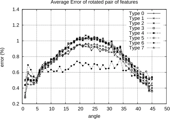
0.2 0.4 0.6 0.8 1 1.2 1.4

0 5 10 15 20 25 30 35 40 45 50

error (%)

angle

Average Error of rotated pair of features

[image:9.612.176.447.426.618.2]

(10)

10 15 20 25 30 35 40 45 50

0 5 10 15 20 25 30 35 40 45 50

error (%)

angle

[image:10.612.177.445.105.301.2]

Figure 12: Maximum error vs angle for Chessboard (normal+45o_PEFs).

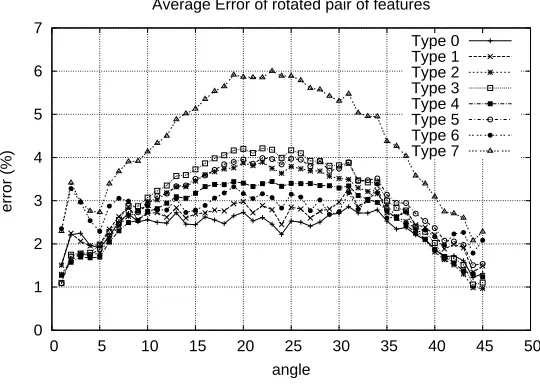
0 1 2 3 4 5 6 7

0 5 10 15 20 25 30 35 40 45 50

error (%)

angle

Average Error of rotated pair of features

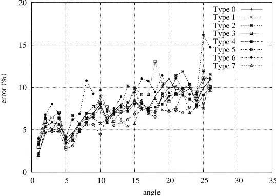
[image:10.612.176.446.427.619.2]

(11)

0 5 10 15 20

0 5 10 15 20 25 30 35

error (%)

angle

[image:11.612.176.445.66.257.2]

Figure 14: Maximum error vs angle for Akiyo (normal+26.5o_PEFs).

image the maximum error was 47% for type 7 features(figure 12). The maximum error in this case almost reached the theoretical value of 50%. The average errors, based on the absolute value of the PEFs, indicate that for most features the PEF values are actually very close to the original feature. For Akiyo, the maximum average error was around 1.1% for feature type 2 (figure 11). For the chessboard the maximum average error was 6% for type 7 features (figure 13).

3.2 Experiment 2: error analysis for PEFs using 0

o

and 26.5

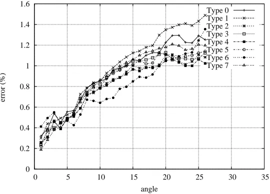
o

In this experiment the third group of features on figure 1 was implemented. Figures 14 and 15 show the maximum errors obtained for Akiyo and for Chessboard. Figures 16 and 17 show the average errors. For some angles the errors improved when comparing to the same angles in experiment 1. The maximum error for Akiyo was 12% for type 3 feature (figure 14). For the chessboard image the maximum error was 34% for type 3 features (figure 15). The maximum errors were close to those obtained in experiment 1. For Akiyo, the maximum average error was around 1.4% for feature type 1 (figure 16). For the chessboard the maximum average error was 6% for type 7 features (figure 17).

However it is clear that the errors at angles around 26o _{should be much smaller. The origin of}

these errors are related to the position calculations during the feature conversion. The positioning of the equivalent features at these angles are much more sensitive than the ones in experiment 1. Any small deviation on one of the points in the Integral Image result in larger errors. The solution for this problem consists in improving the rounding algorithm to consider the best point depending on the circumstances of the area being computed (position, scaling, parity of the coordinates).

4 Conclusions

(12)

0 5 10 15 20 25 30 35 40 45 50

0 5 10 15 20 25 30 35

error (%)

angle

[image:12.612.176.446.106.300.2]

Figure 15: Maximum error vs angle for Chessboard (normal+26.5o_PEFs).

0 0.2 0.4 0.6 0.8 1 1.2 1.4 1.6

0 5 10 15 20 25 30 35

error (%)

angle

[image:12.612.177.447.423.617.2]

(13)

1 1.5 2 2.5 3 3.5 4 4.5 5 5.5 6

0 5 10 15 20 25 30 35

error (%)

angle

[image:13.612.176.446.65.257.2]

Figure 17: Average error vs angle for Chessboard (normal+26.5o_PEFs).

that might affect the accuracy of the classifier. The second experiment showed that although some of the errors are smaller than in experiment 1, the implementation needs some improvement to successfully compute equivalent features at angles of 26.5o_.

The limitations for this approach occur when very long Haar-like features are used to compose a classifier, in which case the errors associated with the PEF are too large to be considered. However it is possible to train classifiers using a more limited set of Haar-like features to avoid this setback. For future work we intend to implement an error correction approach regarding the positioning and sizes of the features that compose a PEF. We are also going to assess and analyse the hit ratios of actual classifiers using the PEF approach.

References

[1] P. Viola and M. Jones, “Rapid object detection using a boosted cascade of simple features,” in CVPR01, pp. I:511–518, IEEE, December 2001.

[2] M. J. Jones and P. Viola, “Robust real-time object detection,” Tech. Rep. CRL-2001-1, Hewlett Packard Laboratories, February 2001.

[3] P. Viola and M. Jones, “Robust Real-Time face detection,” in Proceedings of the Eighth International Conference On Computer Vision (ICCV-01), (Los Alamitos, CA), pp. 747–747, IEEE Computer Society, July 2001.

[4] G. Guo and H. Zhang, “Boosting for fast face recognition,” Tech. Rep. MSR-TR-2001-16, Microsoft Research (MSR), Feb. 2001.

[5] M. Kolsch and M. Turk, “Analysis of rotational robustness of hand detection with a viola-jones detector,” inICPR04, pp. III: 107–110, 2004.

[6] S. Mitri, K. Pervlz, H. Surmann, and A. Nchter, “Fast color-independent ball detection for mobile robots,”Mechatronics and Robotics, pp. 900–905, September 2004.

(14)

[8] M. J. Jones and P. Viola, “Fast multi-view face detection,” Tech. Rep. TR2003-96, MERL, July 2003.

[9] R. Lienhart and J. Maydt, “An extended set of haar-like features for rapid object detection,” in ICIP02, pp. I: 900–903, September 2002.

[10] Y. Freund and R. E. Schapire, “A short introduction to boosting,” Journal of Jap. Society for Art. Intell., vol. 14, no. 5, pp. 771–780, 1999.

[11] R. Lienhart, A. Kuranov, and V. Pisarevsky, “Empirical analysis of detection cascades of boosted classifiers for rapid object detection,” inDAGM03, (Madgeburg, Germany), pp. 297– 304, September 2003.

[12] S. Z. Li and Z. Zhang, “Floatboost learning and statistical face detection,” IEEE Trans. on Pattern Analysis and Machine Intelligence, vol. 26, pp. 1112– 1123, September 2004.