PROXIMATE DETERMINANTS
E
KISAL.
A
NYARA,
A
NDREWH
INDEA
BSTRACTThis paper analyses regional fertility patterns in Kenya since 1989 using data from the four Demographic and Health Surveys of 1989, 1993, 1998 and 2003, and a consistent set of 21 regions. The impacts of late and non-marriage, contraceptive use, sterility and postpartum non-susceptibility on fertility in each region are quantified using the model of the proximate determinants of fertility developed by John Bongaarts. The model is modified to take account of the impact of non-marital childbearing and secondary sterility. Substantial and persistent regional differentials in fertility are identified. Generally, fertility is lowest in urban areas and in rural areas in the centre of the country. It is higher in both coastal and western areas. The pattern of increasing contraceptive use and a rising age at marriage offsetting the impact of shorter durations of breastfeeding as modernisation progresses is only found in a small number of regions in Central and Eastern Provinces, and in Nairobi. Elsewhere a variety of demographic regimes is observed, some associated with fertility decline, others associated with constant or even increasing fertility. There are differences between the experiences of Nairobi and Mombasa, the two largest urban areas, with Mombasa’s low fertility being associated with none of the major proximate determinants.
Fertility transition in Kenya: a regional analysis of the
proximate determinants
Ekisa L. Anyara* Andrew Hinde**
School of Social Sciences and
Southampton Statistical Sciences Research Institute University of Southampton
Southampton SO17 1BJ United Kingdom
* Email: ela@soton.ac.uk
** Email: prah@socsci.soton.ac.uk
Acknowledgements
Abstract
This paper analyses regional fertility patterns in Kenya since 1989 using data from the four Demographic and Health Surveys of 1989, 1993, 1998 and 2003, and a consistent set of 21 regions. The impacts of late and non-marriage, contraceptive use, sterility and postpartum non-susceptibility on fertility in each region are quantified using the model of the proximate determinants of fertility developed by John Bongaarts. The model is modified to take account of the impact of non-marital childbearing and secondary sterility. Substantial and persistent regional differentials in fertility are identified. Generally, fertility is lowest in urban areas and in rural areas in the centre of the country. It is higher in both coastal and western areas. The pattern of increasing contraceptive use and a rising age at marriage offsetting the impact of shorter durations of
1 Introduction
Kenya’s total fertility rate has fallen from 8.1 children in 1978 to 4.9 in 2003. The decline has taken place in both less and more developed regions, among a range of different social and economic groups, and has occurred with a rapidity many did not anticipate. Previous studies (National Council for Population Development (NCPD) 1989, Cross et al. 1991, Brass and Jolly 1993, Macrae et al. 2001, Blacker 2002) have attributed the decline mainly to the increased use of contraceptive methods. The fertility-suppressing effects of postpartum infecundability and late or non-marriage have also been emphasised (African Population and Policy Research Center (APPRC) 1998). Taken together, of course, these three factors constitute the key proximate determinants of fertility (Bongaarts and Potter 1983), and so it would be very surprising if they were not implicated in any major fertility change in a large human population.
This paper has two objectives. The first is to describe regional variations in fertility decline in Kenya since the 1980s. The second is to determine the potential role of the proximate determinants in explaining these regional patterns. The study focuses on the fertility-inhibiting effects of marital patterns, contraception,
postpartum infecundability and sterility. Induced abortion is not examined due to the absence of reliable data.
2 Data
This paper uses individual-level Kenya Demographic and Health Survey (KDHS) data collected in the surveys of 1989, 1993, 1998 and 2003. The KDHSs were organised using the administrative subdivisions of the country into provinces and districts (Figure 1). With the exception of the 2003 survey, they did not include the sparsely populated northern areas of the country, so these are not included in our analysis.
[Figures 1 and 2 about here]
Nairobi. Second, some regions are formed by amalgamating contiguous districts within the same province in order to increase sample sizes and hence the reliability of estimates. These include Nyeri, Nyandarua and Kirinyaga in Central Province; Busia and Bungoma in Western Province; Kitui and Machakos, and Embu and Meru in Eastern Province; Kwale and Kilifi in Coast Province; Laikipia, West Pokot, Elgeyo-Marakwet and Baringo, Kajiado and Narok, and Uasin-Gishu and Trans-Nzoia in Rift Valley Province.
Estimates of fertility and of the proximate determinants for these 21 regions are presented for all four KDHSs with two exceptions. The region of Nandi in Rift Valley Province had a sample in the 1989 survey too small for meaningful analysis. The region of Taita-Taveta in Coast Province was not covered in the 2003 survey, and had only a very small sample in 1989, so we only present results for 1993 and 1998.
The samples in Nairobi and Mombasa regions are largely urban. Kisumu and Nakuru regions have urban samples in all surveys of more than 40 per cent and more than 29 per cent respectively. The remaining regions are predominantly rural.
Some regions are predominantly inhabited by one ethnic group while others, especially the urban ones, are multi-cultural. The population of Coast Province is dominated by the Mijikenda. Eastern Province has four main groups: the Akamba in Machakos, the Meru and Embu in Meru and the Borana in the north. Central Province is inhabited by the Kikuyu. Rift Valley Province is inhabited by the Maa (in
affected to some degree by modernisation. However, attachment to indigenous lifestyles is still particularly strong among the inhabitants of the Coast and Nyanza Provinces.
We measure fertility using a period of four years before each survey to avoid the problem of birth shifting around a point three or five years before the survey date because of the requirement to ask additional questions about births within a three- or five-year window (Institute for Resource Development, 1990). We estimate age-specific fertility rates, total fertility rates, age-age-specific marital fertility rates and total marital fertility rates from survey data using the exact exposure in each age group for each woman during the four years preceding the survey date. Details of the method may be found in Hinde and Anyara (2006).
3 The proximate determinants model
Reproduction among human populations is usually at a level below their fecundity or biological capacity. The actual reproductive performance is influenced by social, economic, cultural, political and environmental factors. The effect of these factors on fertility varies within and between populations and is assumed to be mediated by factors which have a direct impact on fertility. Davis and Blake (1956) developed a set of ideas that showed how both direct and indirect factors are related to fertility. Bongaarts (1978) reorganised the ideas of Davis and Blake and developed the proximate determinants framework and a method for assessing the impact of each proximate determinant on fertility through a set of quantitative indices.
process which involves intercourse, conception and gestation and parturition,
Bongaarts (1982) distinguished four variables that are mainly responsible for fertility variation among populations. These are: the proportion of women married (a measure of exposure to intercourse), contraceptive use (a measure of exposure to conception), induced abortion (a measure of exposure to parturition) and postpartum infecundity or duration of postpartum amenorrhea (also a measure of exposure to conception). Bongaarts et al. (1984) added a fifth major variable, primary sterility (another measure of exposure to conception) to the proximate determinants model.
These five variables were quantified using five indices which measure the fertility reducing effect of the respective proximate determinants: Cm is the index of the proportion married, Cc the index of contraception, Ca the index of abortion, Ci the index of lactational infecundity and Ip or Cp the index of primary sterility. Each index equals the ratio between the fertility levels in the presence and the absence of the inhibition caused by the corresponding proximate fertility variable and takes only values between 0 and 1. A value of 0 means that the determinant completely inhibits fertility while a value of 1 means that it has no effect on fertility. Thus the closer the index is to zero the more influential the associated proximate determinant is in reducing fertility rate from its biological maximum.
hence the TFR will be equal to the total marital fertility rate (TMFR). The degree of fertility reduction arising because not all women of reproductive age are married is measured by the ratio of the TFR and the TMFR, and it is this ratio which Bongaarts defined as Cm. In symbols, therefore
TFR TMFR
m
C = .
If, in addition to being married throughout their reproductive age span, women in a population do not engage in deliberate birth control (whether through contraception or induced abortion), then the fertility of married women would, effectively, be ‘natural’. If we denote the average number of children such women would bear in their lifetimes as the total natural marital fertility rate (TN), then Bongaarts suggested that in the absence of contraception and induced abortion, TMFR = TN and Cc = Ca = 1. The ratio between the TMFR and TN is a measure of the impact of contraception and induced abortion in reducing fertility, so that, in general
TMFR TN
c a
C C = .
Finally, if, in addition, women no longer experienced postpartum infecundity, fertility would rise from its total natural marital level to its biological capacity, TF. The index of postpartum infecundity, Ci, therefore measures the ratio between TN and TF:
TN TF
i
C = .
around this as a result of the effects of differences in the less important proximate determinants of fertility, such as natural fecundability, spontaneous intra-uterine mortality, the extent of permanent sterility, the frequency of intercourse and the duration of the fertile period. Other studies (e.g. Cleland and Chidambaram 1981) found that substantial residual variation exists in total fecundity. Regardless of the level of TF, however, the difference between the observed TFR and TF can always be partitioned into the effects of non-marriage (and marital disruption), the use of
contraceptives and induced abortion and the effect of postpartum infecundity induced by breastfeeding and abstinence (Bongaarts 1982, Bongaarts and Potter 1983) using the equation
TFR (TF)=C C C Cm c a i .
Bongaarts’s model is good at discerning interpopulation variation. It is easy to use with aggregate data and does well in identifying the components of fertility differentials. Since its initial formulation, it has been widely used (APPRC 1998, Jolly and Gribble 1993, Cleland and Chidambaram 1981, Casterline et al. 1983, Kalule-Sabiti 1984) and widely championed (Hobcraft and Little 1984, Palloni 1984, Stover 1998). Its great strength is its easy application using widely available data to decompose the contribution of each of the intermediate variables selected on the current levels of fertility over time and across regions. Nevertheless, some
4 Sterility
Sterility is the condition in which a woman is unable to conceive or a pregnancy does not successfully end in a birth. Usually women are sterile before menarche (the onset of menstruation) and after menopause. After she first menstruates a woman
experiences a period of natural infertility characterised by anovulation or incomplete cycles. This has little effect on fertility because most of this period occurs outside exposure to sexual intercourse.
Primary sterility (the complete inability to have a child) may be due to sexually transmitted diseases. These diseases may also cause secondary sterility (the inability to have more children even though the menopause has not been reached given that at least one child has been born). As mentioned earlier, in later
developments of the model, Bongaarts et al. (1984) added the indexCp, which was intended to measure the fertility-inhibiting impact of sterility. However, this index actually only measures the effect of primary sterility. It is expressed as
Cp = (7.63 - 0.11s)/7.3,
where s is the proportion of ever-married women in the 45-49 (or, in some
applications, the 40-49) year age group who are childless or who have had no live births (Frank 1983).
assumed to be due to pathological sterility and Cp is less than 1, meaning that it has some inhibiting effect on fertility.
The original model considered primary sterility only and did not incorporate the fertility inhibiting effects of secondary sterility, because of the lack of data on the latter. In order to include secondary sterility in the analysis, we use data on the proportion, f, of married women who were sexually active in the month before the survey and who are infecund. This proportion is defined as those sexually active women who are menopausal, not pregnant, and have not had a birth in the last five years, during which period they have never used contraception. Women who are not married, or who have been married for less than one year, or who have not yet experienced menstruation are excluded. The original Cp index can then be replaced by an index of sterility due to any cause, Cs(Stover 1998), which is calculated as
Cs= 1 – f. .
The index Csexpresses the total effect of infecundity on fertility and it takes the value 0 if all sexually active women are infecund and the value 1 (no fertility-reducing effect) when all sexually active women are fecund.
Data sufficient to estimate Cs can be obtained from the Demographic and Health Surveys. However, Ericksen and Brunnette (1996) found that some African women who reported being infecund for the last five years were in that state
the risk of becoming pregnant because they are infertile. Unlike the previous index which was based on a regression of the TFR as a function of the proportion childless, the use of f directly measures the effect of infecundity on fertility.
When the index of sterility due to any cause, Cs, is added to the model, it accounts for some of the total fecundity component, TF. In other words, TF can now be viewed as being the product of some potential fecundity (PF) multiplied by Cs. Therefore the model now becomes
TFR (PF)=C C C C Cm c a i s .
The difference between TF and PF is that PF is a measure of the fertility of the woman in a population if all were fecund until the end of the childbearing age range (typically 50 years), whereas TF takes account of the population-specific sterility measured by Cs.
5 Application of the model to the Kenyan experience
Index of marriage, Cm. In the proximate determinants formulation, the index of
In a population where sexual activity takes place exclusively within marriage, and in which all married couples in which the wife is of childbearing age can be assumed to be sexually active, then the identity between marriage and sexual activity is exact. In such a population, the index Cm can be computed as a weighted average of age-specific proportions married m(a) with the weights given by the age-specific marital fertility rates g(a). In symbols,
( ) ( )
( )
a m
a
m a g a C
g a
=
∑
∑
.In this case, ( )
a
g a
∑
= TMFR and ( ) ( )a
m a g a
∑
= TFR and so( ) ( )
TFR
( ) TMFR
a
a
m a g a
g a =
∑
∑
. (1)More commonly, however, some women who are not married are sexually active, and some women who are married are not sexually active. Consider first non-married women. To the extent that these women have sexual intercourse and bear children, the fertility-inhibiting effect of non-marriage will be attenuated. In populations with positive non-marital fertility, equation (1) no longer holds, and it is more appropriate to obtain Cm directly as the ratio of the TFR (the number of children a woman would bear through out her life time at constant age-specific fertility rates (ASFRs)) to the TMFR (the number of children she would bear at constant age-specific marital fertility rates (ASMFRs) if she first entered into a marriage at age 15 and stayed in it through out her reproductive lifespan) (Bongaarts, 1982).
using the formula
( ) ( )
( )
a
a
m a g a
g a
∑
∑
the resulting index will overestimate thefertility-reducing effect of late and non-marriage. In such a context, Jolly and Gribble (1993) suggested defining two indices of the impact of late and non-marriage on fertility:
TFR TMFR
m
C = ,
and ( ) ( ) * ( ) a m a
m a g a C
g a
=
∑
∑
.It turns out (see Appendix) that
TUFR *
TMFR
m
C = ,
where TUFR is the total union fertility rate, and is the sum of the age-specific union fertility rates (ASUFRs) over all the childbearing ages. The ASUFR for age group a
is equal to the number of births to married women in age group a divided by the person years lived by all women in age group a. In other words, it is a measure of the fertility rate that would have obtained at age a if there had been no fertility outside marriage.
The relationship between Cm and Cm* is measured by an additional parameter, which Jolly and Gribble (1993) termed M0, defined so that
0 * m m C M C = .
When so defined, M0 also measures the ratio between the TFR and the TUFR (see
approximately 23 per cent higher than it would have been if there were no fertility outside marriage. If fertility only occurs within marriage, then M0 = 1. According to
these definitions, therefore, Cm measures the actual fertility-inhibiting effect of late and non-marriage in the population under study after taking into account fertility outside marriage, and Cm* measures what the impact of late and non-marriage on fertility would have been if there had been no births outside marriage.
Consider now those women who are married but who are not sexually active. To the extent that married women are not sexually active then the fertility-inhibiting effect of late marriage and non-marriage will be reduced. However, there are both theoretical and practical difficulties with adjusting the model to account for this. It is known that in historical populations, abstinence from sexual intercourse was used as a method of contraception, and the practice is credited to have been one of the movers of fertility decline in England and Wales in the late nineteenth and early twentieth centuries when couples took steps to reduce numbers of conceptions in response to the increased ‘perceived relative cost’ of childbearing (Szreter 1996). Therefore unless information on the motivation for a lack of sexual activity on the part of married women is available, treating it as an ‘exposure’ factor is problematic. The Demographic and Health Surveys (DHSs) do not provide this information.
information, such as the TMFR, which is useful for cross-cultural comparisons. Second, marriage is pervasive in Kenya. The institution of marriage confers legality on sexual relationships and ensures the social legitimacy of the children born as a result of those relationships. The use of s(a) ignores the important role of marriage as a social institution in patterning fertility. Third, as we have already mentioned, among married women the way this variable is typically measured in DHSs, which is on the basis of whether or not each respondent has been sexually active in the
preceding month has the danger of confusing periods of sexual abstinence with contraception. Fourth, the use of s(a) would not provide us with information on the proportion of total fertility that is accounted for by births outside marriage. The use of the measures Cm and Cm* as described above achieves this, and also allows us to measure the effective fertility resulting from sexual activity before marriage.
The effect of this is that children born to women who are married at the survey date during a previous marital disruption are classified as occurring in the union extant at the survey date. The opposite misclassification applies to children born to women who were divorced or widowed at the time of the survey but who were married at the time of the birth of the children. It is expected that these effects will roughly cancel out. If disruptions due to divorce or widowhood are relatively rare then it is believed that their effect on the accuracy of the estimates will be small, and the currently married women represent a group with a more or less stable
exposure to the risk of conception (United Nations 1983).
The index of noncontraception, Cc. Bongaarts (1978) considered contraception as
any deliberate parity-dependent practice including abstinence and sterilisation undertaken to reduce the risk of conception. In the later modification contraception referred to any deliberate practice aimed at limiting family size and excluded breastfeeding and postpartum abstinence because these two aim at promoting
maternal health and child development rather than regulating the number of children born (Bongaarts et al. 1984). The index of contraception, Cc, is intended to estimate the effect of contraception on marital fertility, assuming that induced abortion is absent. Ccis estimated using the equation
Cc = 1 - 1.08ue, (2)
e(m) for each method m, with weights equal to the proportion of women using each given method (Bongaarts 1982, Bongaarts and Potter 1983). The term 1.08 is a correction or adjustment factor for the concentration of contraception among non-sterile women once women who believe they are non-sterile stop using contraception (Nortman 1980). It serves the purpose of removing infecund women from the equation so that Cc becomes zero if effective prevalence reaches 92.5 per cent in which case the remaining women would be presumed to be infecund (Stover 1998).
The proximate determinants model assumes that each of the determinants has an independent inhibiting effect on fertility. However, the assumption that only fecund women use contraceptives has been questioned (Reinis 1992; Stover 1998). It is argued that in the age-group 45-49 years an estimated 52 per cent of women are infecund. This suggests that an overlap between contraception and infecundity may exist, since many women at older childbearing ages who are using sterilisation and other similar long-term methods are likely to be infecund, a problem acknowledged by Bongaarts and Potter (1983). A similar overlap may occur between contraception and postpartum amenorrhea, although this has been found to be low in most countries (Thapa et al., 1992, Stover 1998, Curtis 1996, Laukaran and Winikoff 1985).
The problem of infecund women also being sterilised is overcome by adding to the model the index of sterility, Cs. This is the approach adopted in this paper. When the index of sterility is added to the model, the correction factor of 1.08 is no longer needed in the equation for Cc, which becomes
Cc = 1 – ue, (3)
(1993) to account for an expanded range of methods. The modification made by Jolly and Gribble involved separating the methods in the ‘other’ category into ‘other modern methods’ and ‘traditional methods’. The use effectiveness of ‘traditional’ methods is reduced to 0.3 in Jolly and Gribble (1993) from a value of 0.7 allocated by Bongaarts and Potter (1983). The revision downplays the effectiveness of
non-modern methods and obscures the potential effectiveness of abstinence. The use of abstinence as a family planning method is not emphasized in Kenya. Unfortunately this negatively affects the promotion of sexual abstinence which turns out to be the most efficient method in the fight against HIV/AIDS in Kenya (Anyara 2000). The values of e(m) used in our analysis are as follows: pill, 0.90; intra-uterine device, 0.95; sterilisation, 1.00; other ‘modern’ methods (injectables, Norplant, condom and diaphragm/foam/jelly), 0.70; and ‘traditional’ methods, 0.30.
Index of postpartum infecundability, Ci. The index of postpartum infecundability,
measures the effect of extended periods of postpartum amenorrhea on fertility. In the original model, Ci referred to lactational infecundability only. Bongaarts (1982) incorporated postpartum abstinence into the index, and Ci became the index of postpartum infecundability and is the ratio of total natural fertility to total fecundity.
duration of postpartum anovulation will lengthen the average birth interval by i
months resulting in a total birth interval of 18.5 + i months, where i is determined by the duration and intensity of suckling. Thus in the presence of breastfeeding the average birth interval equals 18.5 months plus the total duration of the infecundable period caused by postpartum amenorrhea and sexual abstinence . The
fertility-reducing effect of breastfeeding, Ci, is then expressed as the ratio of the average birth interval in the absence of breastfeeding to the average birth interval in the presence of breastfeeding plus post partum non-susceptibility. This is symbolically written
Ci=
i
+
5 . 18
20 .
The value of i can be derived as a ratio of prevalence (the number of married women amenorrheic or abstaining whichever is longer at the time of the survey) to incidence (average number of births per month to married women in a given window in
months) (Jolly and Gribble 1993, APPRC 1998). However, in the absence of information on amenorrhea most previous estimates of the mean or median duration of breastfeeding were made using the equation
2
= 1.753exp(0.1396 0.001872 )
i B− B , (4)
whereB is the mean or median duration of breastfeeding in months (Bongaarts 1982; Bongaarts and Potter, 1983). Often DHS data produce distributions of the duration of breastfeeding that are highly skewed. Consequently the median duration of
model is an aggregate model and other indexes of the model are based on means or proportions.
Now that data on amenorrhea are available, we have used the mean duration of postpartum non-susceptibility derived using current status data on lactation for women who are amenorrheic plus those abstaining to represent i. This is a combined effect of both postpartum abstinence and amenorrhea and it is a complete measure of the fertility reducing effect of the postpartum period. In this analysis,Ci is redefined from being the index of the fertility inhibiting effect of lactational infecundability or postpartum infecundability to the fertility inhibiting effect of postpartum
non-susceptibility.
Index of induced abortion, Ca. The contribution of induced abortion to fertility
reduction in Kenya is not examined in the current study due to lack of data. The practice is illegal in Kenya and can only be done in hospitals in very exceptional circumstances. Illegal abortions do appear to be practiced, as evidenced by the appearance of patients with abortion complications in urban hospitals. But official data on this are lacking and the collection of data on it was not attempted in the first two Kenyan DHSs. In the 1998 and 2003 Kenyan DHSs a question on induced abortion was asked indirectly. For example in 2003 the women were asked: have you ever had a pregnancy that miscarried, aborted or ended in a stillbirth. The response to this question did not specifically target induced abortion.
per year at this hospital. Our estimates of the total natural marital fertility (TN) and potential fecundity (PF) are biased downward due to the fact that we cannot take abortion into account.
6 Results
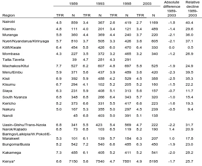
Fertility decline. Kenya’s fertility has declined by 39 per cent since 1978 and by 26 per cent since 1989. A decline has occurred in all regions with exception of
Narok/Kajiado and Baringo/Laikipia/West Pokot/East Marakwet (which, for
convenience, is hereafter referred to simply as ‘Baringo’) (Table 1). Since 1989, the largest declines of over 35 per cent have occurred in Muranga,
Nyeri/Nyandarua/Kirinyaga, Nairobi, Meru/Embu and Kisii regions followed by 32 per cent in Uasin-Gishu/Trans-Nzoia. All these regions are located in the highland areas of Kenya. The Kilifi/Kwale region in Coast Province experienced almost no decline. Narok/Kajiado and Baringo regions, which are inhabited by pastoral
communities, reported fertility gains of 21 and 18 per cent respectively between 1989 and 2003.
[Table 1 about here]
low and based on a very small sample. Between 1993 and 1998 rapid decline was sustained in Machakos/Kitui region, but apart from this, regions where fertility had declined fastest between 1989 and 1993 experienced a slowing down in the rate of decline (for example Muranga). During the period 1993-1998 the most rapidly declining fertility was observed in Meru/Embu, Kisii, and Nandi regions. Between 1998 and 2003 the decline in fertility ceased at the national level, and this stagnation was reflected in almost all regions. Only in Muranga, South Nyanza (for the first time) and Uasin-Gishu/Trans-Nzoia was there any substantial decline during this period and large gains in fertility of 20 per cent and over were recorded in Machakos, Narok/Kajiado and Kericho regions.
Throughout the period, the lowest fertility was reported in the major urban regions of Nairobi and Mombasa, but the rate of decline in Nairobi exceeded that in Mombasa, so that whereas Mombasa had the lowest total fertility rate (TFR) in
Kenya in 1989 its rate of decline between 1989 and 2003 was lower than that reported in some of the rural districts.
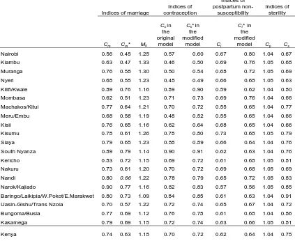
The proximate determinants indices. We have calculated the proximate determinants indices using both the original formulation of the model and in the modified version used in this paper for each region of Kenya in 2003 (Table 2). The indices of marriage show a consistent relationship to one another. A value of 1.18 for
M0 implies that roughly 18 per cent of fertility in Kenya takes place outside marriage
(see Appendix). The regional figures for M0 reveal that this proportion does not vary
regional patterning in the two indices of marriage is roughly the same. Late and non-marriage has the greatest impact in the cities of Nairobi and Mombasa, in the Central Province regions of Kiambu and Nyeri/Nyandarua/Kirinyaga, and in the adjacent Meru/Embu region in Eastern Province. Its impact is least in rural areas of Coast Province (Kilifi/Kwale region), South Nyanza and the pastoral region of
Narok/Kajiado. [Table 2 about here]
The relationship between the two indices of the impact of contraceptive use on fertility is straightforward. Comparing equations (2) and (3) above reveals that the modified index should be slightly greater than that in the original model, because the term subtracted from 1 is less by a factor of 1.08. This is indeed what we find in all regions (Tables 3-6).
Turning now to the index of post-partum non-susceptibility, we find that in general, the modified version of the index is greater than the original one calculated using equation (4). The difference is greatest in Nairobi, Machakos/Kitui and Meru/Embu regions. There are a few regions, however, where the reverse is true, notably South Nyanza on Lake Victoria and the Narok/Kajiado region. It turns out that the mean duration of breastfeeding represented by B in equation (4) is often longer than the mean duration of non-susceptibility, i. This in most cases results in the index generated using the equation being lower.
The original index of sterility, Cp, varies little from region to region, and is greater than 1, implying that primary sterility in Kenya is very rare. The index Cs, which measures the current effect of infecundity on exposure to the risk of
on overall fertility. The impact of infecundity is least in the pastoral areas of Rift Valley Province (Narok/Kajiado and Baringo) and areas of Western Province
(Bungoma/Busia) and greatest in the regions of Central Province (Kiambu, Muranga and Nyeri/Nyandarua/Kirinyaga), the adjacent Meru/Embu region in Eastern
Province, and the urban areas of Nairobi, Mombasa, Kisii and Nakuru.
The revised set of indices provides a more complete and informative picture of the proximate determinants of fertility than the original indices, so we use only the revised indices in the remainder of this paper.
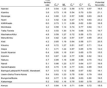
The role of the proximate determinants in Kenya, 1989-2003. In 1989, when the total fertility rate (TFR) was 6.6, the most important of the proximate determinants in inhibiting fertility was post-partum non-susceptibility (Table 3). Over the subsequent 14 years, its impact changed little at the national level (Tables 4-6), with the index Ci rising from 0.63 to 0.64. Ignoring variation which is accounted for by the small numbers of women in some regions, the regional pattern also exhibited little change, with the effect of postpartum non-susceptibility generally being greatest in rural areas, and least in the towns and cities. Despite the decline in fertility between 1989 and 2003, the impact of (principally) breastfeeding in increasing the length of birth intervals remains important.
[Tables 3-6 about here]
Mombasa. There are certain rural areas, too, where nuptiality has fallen substantially, notably Uasin-Gishu/Trans-Nzoia in Rift Valley Province (the fall here being mainly between 1989 and 1993) and Nyeri/Nyandarua/Kirinyaga in Central Province. There is a more consistent pattern in the proportion of fertility occurring outside marriage. This changed little at the national level over the period between 1989 and 2003, and regional patterns largely persisted too, with relatively high proportions in Nairobi, Central Province, the regions of Eastern Province which border Central Province (Meru/Embu and Machakos), Nakuru in Rift Valley Province, and, from 1993 onwards, Kisumu and Siaya in Nyanza Province (Tables 3-6). The regions where most childbearing occurs within marriage and where fertility inhibition due to non-marriage is low were mostly in Western and Rift Valley provinces, but also include Kilifi/Kwale in Coastal Province.
The fertility-reducing effect of contraceptive use increased between 1989 and 2003 (though there has been no change since 1998). The geographical pattern in 1989 was rather curious, in that the lowest values of the index Cctended to be in some of the more developed rural areas, such as Nyeri/Nyandarua/Kirinyaga and Meru/Embu, rather than in the major towns and cities, and there were generally low levels in Central Province. Significantly, the city of Mombasa had a relatively high value of Cc of 0.80 (Table 3). Contraceptive use had little impact in Nyanza and Western Provinces. Between 1989 and 1993 there were slight changes to this pattern, notably the addition of Kisii region in Nyanza Province to the list of areas where contraceptive use had a substantial impact (Table 4). Between 1993 and 2003,
Central Province, Meru/Embu in Eastern Province and Kisii in Nyanza Province. On the other hand, it reduced fertility by 20 per cent or less in Kilifi/Kwale in Coastal Province, all of Nyanza Province except Kisii region, and Baringo region in Rift Valley Province (Tables 4-6). It continued to have less impact in the city of Mombasa than might be expected from the latter’s status as a large urban area. In general, therefore, contraceptive use in Kenya has its greatest impact on fertility in the centre of the country, and its impact becomes less as we move away from the centre to the east and west.
Between 1989 and 2003, the impact of infecundity in reducing fertility rose moderately, though geographical patterns were, for the most part preserved. Infecundity is lowest in the Rift Valley Province regions of Narok/Kajiado and Kericho, and in Western Province; it is highest in Central Province and Nairobi. There are distinctive patterns in two regions. In Mombasa, infecundity has a large effect in reducing fertility throughout the period; and in Kisii region (and, to a lesser extent Nakuru), its impact has been increasing since 1989.
with numbers ranging from below 14 births to over 23 births (Tables 3-6). However, there is also a striking amount of consistency in the regional pattern. For example, several regions, notably Nyeri/Nyandarua/Kirinyaga and Meru/Embu have
consistently high values (in excess of 21 births in all years, and up to 25 births in certain years). Elsewhere there are low values in all four years: for example in Siaya and Kisumu regions in Nyanza Province, and the city of Mombasa. The PF in other regions tends to fluctuate, though it is high in Kisii and Mackahos/Kitui regions from 1993 onwards. The semi-arid region of Narok/Kajiado shows a persistent increase in PF from 14.5 in 1989 to 23.4 in 2003.
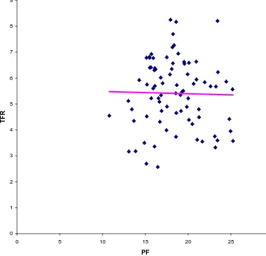
Although PF varies among the regions, a scatter plot of the relationship between PF and the TFR (Figure 3) shows that there is almost no correlation between the two variables (r = 0.02). This suggests that almost all the systematic variation in the TFR is captured by the proximate determinants considered in the analysis and that PF is operating in the model as a random error term.
[Figure 3 about here]
The relationship of the proximate determinants to fertility. We can examine the relationship between the proximate determinants and fertility outcomes in more than one way. One approach is to examine how changes in the proximate determinants, as measured by the set of indices we have calculated, have effected the overall change in the total fertility rate (TFR) in Kenya (Table 7). Between 1989 and 1993 the TFR fell by 1.0 births, from 6.6 to 5.6. The biggest contributor to this change was an increase in contraceptive use, although changes in the other proximate determinants
However, here the biggest single contribution was a change in potential fecundity, followed by a fall in sterility. Contraceptive use only contributed 0.3 births to the fall, and this was more than outweighed by changes in postpartum non-susceptibility. Between 1998 and 2003 the TFR changed little, and neither did any of the proximate determinants. The most interesting conclusion to be drawn from this analysis is that the impact of contraceptive use on Kenyan fertility has been falling since the early 1990s.
[Table 7 about here]
An alternative way of looking at how the proximate determinants relate to fertility is to plot the values of each index against the TFR across all regions, pooling the data from the four surveys (Figure 4). The relationship between contraceptive use, late and non-marriage and sterility is as expected: as these increase, the TFR falls. But the bivariate relationship between postpartum non-susceptibility and the TFR is in the other direction. Regions with longer periods of postpartum non-susceptibility have higher fertility, other factors being held constant. This paradoxical result arises because other factors are not constant: long periods of
postpartum non-susceptibility are characteristic of rural areas where marriage ages are low and contraceptive use is minimal.
[Figure 4 about here]
7 Discussion
since the 1980s. Kenya‘s fertility experienced a rapid decline up to the early 1990s but then started to stagnate in some regions and even to rise in others in the second half of the 1990s (APPRC 1998; Macrae et al., 2001). While the social, economic and cultural reasons behind the stagnation and increase in Kenya need to be investigated, this trend of fertility behavior has been documented in Botswana (Boserup 1985, Easterlin and Crimmins 1985), and Ghana (Onuoha and Timaeus 1995).
Increases in fertility levels were experienced in the Narok/Kajiado and Baringo regions which are predominantly inhabited by the pastoral communities of the Maa and Kalenjin. It is not clear whether the environmental pressures arising from arid and semi-arid conditions of these regions whose inhabitants widely practice an early age at marriage influenced the observed fertility. In fact, in Narok/Kajiado region the increase was mainly the result of a rise in potential fecundity, and so is not easily explained by changes in the major proximate determinants (late and non-marriage, contraception and postpartum non-susceptibility).
Kisii regions. It is this last group of areas in which contraceptive use and a rising age at marriage have had the biggest impact on the fertility decline. The usual description of the Kenyan fertility transition as being driven by a rising age at marriage and increased contraceptive use (Brass and Jolly 1993, Macrae et al. 2001) seems to apply here. However, even in Nairobi and the regions of Central Province, the ‘classic’ pattern by which increased contraception offsets the impact of declining durations of postpartum non-susceptibility is only evident between 1993 and 1998.
Uasin-Gishu/Trans-Nzoia in Rift Valley Province and Meru/Embu in Eastern Province are the two regions in which fertility decline seems to have been sustained throughout the period between 1989 and 2003. Uasin-Gishu/Trans-Nzoia is a region of net in-migration (Central Bureau of Statistics, 2002) but it is the only region in Rift Valley which experienced a substantial fertility decline. It is a region containing land with high agricultural potential and since the end of the colonial period it has
attracted wealthy migrants. The effects on fertility arising from migration might depend on the socio-economic level of both the in-migrants and the receiving population. Meru/Embu might best be considered along with Kiambu and
Nyeri/Nyandarua/Kirinyaga regions. These three regions are all located in the Kenya highlands and have a high Human Development Index (UNDP 2002). Finally, we can consider Nairobi and Mombasa, the two largest urban areas in the country. They both have low and declining fertility, though the decline has stagnated since 1998. However, there is an interesting difference between the two in the impact of
There are a few other regions with distinctive fertility trends. One of the most striking is Kilifi/Kwale region in Coast Province, where fertility has changed little. This rural area seems to have a distinctive and unchanging demographic regime characterised by relatively low nuptiality which is compensated for by fertility outside marriage, long periods of postpartum non-susceptibility (both of which tend to reduce fertility), very low contraceptive use and low sterility (both of which tend to raise fertility). Kisii region has a fertility experience which is different from that of the rest of Nyanza Province, a feature which may be associated with its different ethnicity.
8 Conclusion
Fertility declined in Kenya by 39 per cent between 1978 and 2003. We have been able to establish the existence of regional differentials in the decline. Since 1998 the decline has stagnated in some regions but the possibility of continued decline is held out by the continued steady downward trend of fertility in some regions.
In general, the fertility inhibiting effects of the proximate determinants in births per woman vary across regions. The inhibiting effects of non-marriage and sterility due to any cause have tended to increase with time and are high in urban areas and regions with low fertility. Births outside marriage account for a substantial proportion of total fertility in Central Province, adjacent areas of Eastern Province and urban regions.
Increased contraceptive use was the most important determinant of fertility change between 1989 and 1993, but its impact on the Kenyan fertility decline seems to have become much more muted since 1993. Relatively few regions of Kenya display a pattern of increased contraceptive use and a rising age at marriage
compensating for declining durations of breastfeeding. Elsewhere there are a variety of patterns and pathways by which the proximate determinants influence fertility. In particular, the low fertility of the urban area of Mombasa is not fully explained by the levels of the major proximate determinants.
The estimates of the impact of the proximate determinants that have been presented are affected by errors in the reporting of the duration of postpartum
abstinence, age at marriage, use of contraception and current age as well as by errors associated with measurement of variables and the fitting of the proximate
Appendix. The interpretation of Cm, Cm* and M0
Let the number of married women at age a be Wm(a), and the number of unmarried women at age a be Wu(a). Let the number of births to married and unmarried women at age a be Bm(a) and Bu(a) respectively. Then the total fertility rate (TFR) is given by the equation
a ( ) ( ) TFR = ( ) ( ) m u m u
B a B a
W a W a
⎛ + ⎞
⎜ + ⎟
⎝ ⎠
∑
and the total marital fertility rate (TMFR) is given by the equation
a ( ) TMFR = ( ) m m B a W a ⎛ ⎞ ⎜ ⎟ ⎝ ⎠
∑
.Therefore if TFR
TMFR
m
C = , we can write
a a ( ) ( ) ( ) ( ) ( ) ( ) m u m u m m m
B a B a
W a W a
C B a W a ⎛ + ⎞ ⎜ + ⎟ ⎝ ⎠ = ⎛ ⎞ ⎜ ⎟ ⎝ ⎠
∑
∑
.We also have
( ) ( ) ( ) ( ) ( ) ( ) ( ) ( ) ( ) ( ) * ( ) ( ) ( ) ( ) ( )
m m m
a m u m a m u
a m
m m
a
a m a m
W a B a B a
m a g a
W a W a W a W a W a
C
g a B a B a
W a W a
⎛ ⎞⎛ ⎞ ⎛ ⎞ ⎜ + ⎟⎜ ⎟ ⎜ + ⎟ ⎝ ⎠⎝ ⎠ ⎝ ⎠ = = = ⎛ ⎞ ⎛ ⎞ ⎜ ⎟ ⎜ ⎟ ⎝ ⎠ ⎝ ⎠
∑
∑
∑
∑
∑
∑
.TUFR *
TMFR
m
C = .
Since the denominators of Cm and Cm* are the same, we can also write
a ( ) ( ) ( ) * ( ) ( ) ( ) ( ) m
a m u
m
m m u
m u
B a
W a W a
C
C B a B a
W a W a
⎛ ⎞ ⎜ + ⎟ ⎝ ⎠ = ⎛ + ⎞ ⎜ + ⎟ ⎝ ⎠
∑
∑
= TUFRTFR = 0
1 M . Therefore 0 TFR . TUFR M =
M0 may be interpreted as an indication of the proportion of all fertility which occurs
outside marriage. For TUFR
TFR = 0
1
M is the ratio between the number of children the average woman would have in her life, ignoring the births outside marriage, and the corresponding number including all births. This is an estimate of the proportion of
fertility which takes place within marriage, and consequently
0
1 1
M
− is an estimate of
References
African Population and Policy Research Center (APPRC) (1998) Fertility decline in Kenya: level, trends and differentials (Nairobi, Population Council, African
Population and Policy Research Center).
Anyara, L.E. (2000) ‘The moral and medical supports of the Catholic Church policy on birth control’. In Kenya’s population prospects: now and beyond (occasional publication no. 1) (Nairobi, Population Association of Kenya).
Blacker, J. (2002) ‘Kenya’s fertility transition: how low will it go?’ In United Nations, Completing the fertility transition (New York, United Nations).
Bongaarts, J. (1978), ‘A framework for analyzing the proximate determinants of fertility’, Population and Development Review 4, 105-132.
Bongaarts, J. (1982), ‘The fertility inhibiting effects of the intermediate variables’,
Studies in Family Planning 13, 179-189.
Bongaarts, J. and Potter, R.G. (1983) Fertility, biology, and behaviour: an analysis of the proximate determinants (New York: Academic Press).
Boserup E. (1985) ‘Economic and demographic relationships in sub-Saharan Africa’,
Population and Development Review 11, 383-397.
Brass, W. and Jolly, C. (eds) (1993) Population dynamics of Kenya (Washington DC, National Academy Press).
Casterline, J.B., Cleland, J. and Singh, S. (1983) ‘The proximate determinants of fertility: cross-national and sub-national variations’, paper presented at the Annual Meeting of the Population Association of America, Pittsburgh.
Central Bureau of Statistics (2002) Kenya 1999 population and housing census: analytical report on population dynamics volume III (Central Bureau of Statistics, Nairobi).
Cleland, J.G., and Chidambaram, V.C. (1981) ‘The contribution of the World Fertility Survey to an understanding of the fertility determinants and trends’, paper presented at the General Meeting of the International Union for the Scientific Study of Population, Manila.
Cross, A., Walter, R. and Kizito, P. (1991) ‘Evidence of transition to lower fertility in Kenya’, International Family Planning Perspectives 17, 4-7.
contraceptive failure rates’, Demography 33, 24-34.
Davis, K. and Blake, J. (1956) ‘Social structure and fertility: an analytical framework’, Economic Development and Cultural Change 4, 211-235.
Easterlin, R.A. and Crimmins, E.M. (1985) The fertility revolution: a supply-demand analysis (Chicago, University of Chicago Press).
Ericksen, K. and Brunnette, T. (1996) ‘Patterns and predictors of infertility among African women: a cross-national survey of 27 nations’, Social Science and Medicine
42, 209-220.
Frank, O. (1983) ‘Infertility in sub-Saharan Africa: estimates and implications’,
Population and Development Review 9, 137-144.
Hinde, A. and Anyara, E.L. (2006) ‘Estimating and analysing current fertility with Demographic and Health Survey data’, paper presented at a workshop at the Population Research Centre, University of Groningen, Netherlands, 2-3 February 2006.
Hobcraft, J. and Little, R.J.A (1984) ‘Fertility exposure analysis: a new method for assessing the contribution of proximate determinants to fertility differentials’,
Institute of Resource Development (1990) An assessment of DHS Data - 1 data quality (Demographic and Health Surveys Methodological Reports No. 1) (Columbia, MD: Institute for Resource Development/Macro Systems Inc.).
Jolly, C.L. and Gribble, J.N. (1993) ‘The proximate determinants of fertility’. In National Academy of Sciences, Demographic change in sub-Saharan Africa
(Washington DC, National Academy Press) 68-116.
Kalule-Sabiti, I. (1984) ‘Bongaarts’ proximate determinants of fertility applied to group data from the Kenya fertility survey 1977/78’, Journal of Biosocial Science 16, 205-218.
Laing, J (1978) ‘Estimating the effects of contraceptive use on fertility’, Studies in Family Planning 9, 150-175.
Laukaran, V.H. and Winikoff, B. (1985) ‘Contraceptive use, amenorrhea, and breastfeeding in postpartum women’, Studies in Family Planning 16, 293-301.
Macrae, S.M., Bauni, E.K., and Blacker, J.G.C. (2001) ‘Fertility trends and
Menken, J. (1984) ‘Estimating proximate determinants: a discussion of three methods proposed by Bongaarts, Hobcraft and Little and Gaslonde and Carrasco’, paper prepared for the International Union for the Scientific Study of Population seminar on Integrating Proximate Determinants into Analysis of Fertility Levels and Trends (London: International Union for the Scientific Study of Population and World Fertility Survey).
National Academy of Sciences (NAS) (1993) Demographic effects of economic reversals in sub-Saharan Africa (Washington DC, National Academy Press).
National Council for Population Development (NCPD) (1989) Kenya Demographic and Health Survey 1989 (Nairobi, Ministry of Planning and National Development).
Nortman, D. (1980) ‘Voluntary sterilization: its demographic impact in relation to other contraceptive methods’, Papers of the East-West Population Institute, no. 65 (Honolulu, East-West Population Institute).
Onuoha, N.C. and Timaeus, I.M. (1995) ‘Has fertility transition begun in West Africa?’, Journal of International Development <<ADD REFERENCE>>.
Reinis, K. (1992) ‘The impact of the proximate determinants of fertility: evaluating Bongaarts’s and Hobcraft and Little’s methods of estimation’, Population Studies 46, 309-326.
Robinson, W.C. and Harbison, S.F. (1993) ‘Components of fertility decline in Kenya: Prospects for the future’. Population Research Center Working Paper (University Park, PA: Pennsylvennia State University).
Stover, J. (1998) ‘Revising the proximate determinants of fertility framework: what have we learnt in the past 29 years?’ Studies in Family Planning 20, 255-267.
Szreter, S. (1996) Fertility, class and gender in Britain 1860-1940 (Cambridge, Cambridge University Press).
Thapa, S., Kumar S., Cushing, J. and Kennedy, K. (1992) ‘Contraceptive use among postpartum women: recent patterns and programmatic implications’, International Family Planning Perspectives 18, 83-92.
UNDP (2002) Kenya human development report 2001 (Nairobi, UNDP).
Table 1
Total fertility rate by region, Kenya 1989-2003
1989 1993 1998 2003
Region TFR N TFR N TFR N TFR N
Absolute difference 1989-2003 Relative decline 1989-2003
Nairobi 4.5 859 3.4 367 2.6 419 2.7 1169 -1.8 40.4
Kiambu 4.8 111 4.0 201 3.4 121 3.4 489 -1.4 29.6
Muranga 5.8 360 4.4 369 4.4 240 3.7 220 -2.1 36.0
Nyeri/Nyandarua/Kirinyaga 5.7 810 3.7 505 3.3 426 3.6 605 -2.1 37.1
Kilifi/Kwale 6.4 454 5.8 426 6.0 470 6.4 330 0.0 0.5
Mombasa 4.3 227 3.5 372 3.2 465 3.2 340 -1.2 26.9
Taita-Taveta 39 4.7 281 4.3 291
Machakos/Kitui 7.7 527 6.2 607 4.8 697 5.8 525 -1.9 24.9
Meru/Embu 5.9 371 5.6 437 3.9 489 3.6 420 -2.3 39.5
Kisii 6.9 392 5.9 488 4.2 529 4.5 388 -2.5 35.3
Kisumu 6.7 294 4.1 102 5.2 205 5.2 160 -1.5 22.2
Siaya 6.3 231 5.9 408 5.1 313 5.6 157 -0.7 11.7
South Nyanza 6.8 348 6.8 266 6.4 343 5.7 320 -1.0 15.4
Kericho 8.2 373 6.6 331 5.5 417 6.6 223 -1.6 19.3
Nakuru 5.0 167 5.3 355 5.0 297 4.5 239 -0.5 9.4
Nandi 45 6.8 403 5.0 391 5.1 138
Uasin-Gishu/Trans-Nzoia 6.8 341 5.5
423 5.4 569 4.7 222 -2.2 31.7 Narok/Kajiado 6.8 73 6.8 103 6.5 119 8.2 190 1.4 20.9
Baringo/Laikipia/W.Pokot/E-Marakwet 5.3 101 6.1 139 5.7 184 6.3 207 1.0 17.8
Bungoma/Busia 8.2 542 7.2 540 6.6 485 6.3 450 -1.9 23.0
Kakamega 7.3 485 6.1 405 5.2 411 5.2 541 -2.0 28.2
Kenya* 6.6 7150 5.6 7540 4.7 7881 4.9 8195 -1.7 25.7
Note: Regional samples do not sum to the national sample in 1993 due to omission of 12 responses from other districts in Coast Province. The same applies to the 2003 national sample where samples from North Eastern Province and some parts of the Rift Valley Province were omitted due to inconsistent coverage.
Table 2
The proximate determinants indices by region, Kenya 2003
Indices of marriage
Indices of contraception Indices of postpartum non-susceptibility Indices of sterility
Cm Cm* Mo
Ccin
the original
model
Cc*in
the modified
model Ci
Ci* in
the modified
model Cp Cs
Nairobi 0.56 0.45 1.25 0.57 0.60 0.67 0.80 1.04 0.67
Kiambu 0.63 0.47 1.33 0.46 0.50 0.69 0.76 1.05 0.68
Muranga 0.76 0.58 1.30 0.50 0.54 0.68 0.72 1.05 0.69
Nyeri 0.68 0.55 1.23 0.45 0.49 0.66 0.68 1.05 0.63
Kilifi/Kwale 0.89 0.76 1.16 0.89 0.90 0.59 0.62 1.04 0.80
Mombasa 0.62 0.51 1.23 0.71 0.73 0.69 0.76 1.04 0.66
Machakos/Kitui 0.77 0.64 1.21 0.70 0.72 0.55 0.65 1.04 0.77
Meru/Embu 0.68 0.58 1.19 0.48 0.52 0.55 0.65 1.04 0.66
Kisii 0.76 0.65 1.16 0.62 0.64 0.68 0.65 1.04 0.66
Kisumu 0.78 0.61 1.26 0.78 0.80 0.73 0.68 1.05 0.79
Siaya 0.79 0.65 1.23 0.88 0.89 0.66 0.64 1.04 0.76
South Nyanza 0.89 0.79 1.14 0.90 0.91 0.62 0.63 1.04 0.76
Kericho 0.83 0.72 1.15 0.69 0.72 0.61 0.68 1.05 0.81
Nakuru 0.73 0.61 1.20 0.70 0.72 0.69 0.68 1.05 0.69
Nandi 0.80 0.66 1.22 0.78 0.79 0.65 0.72 1.05 0.83
Narok/Kajiado 0.90 0.77 1.16 0.82 0.83 0.57 0.56 1.05 0.85
Baringo/Laikipia/W.Pokot/E.Marakwet 0.80 0.73 1.09 0.84 0.85 0.61 0.63 1.04 0.91
Uasin-Gishu/Trans Nzoia 0.70 0.57 1.22 0.72 0.74 0.65 0.67 1.04 0.72
Bungoma/Busia 0.77 0.69 1.12 0.76 0.78 0.61 0.68 1.04 0.86
Kakamega 0.79 0.69 1.15 0.72 0.74 0.63 0.66 1.05 0.81
Kenya 0.74 0.63 1.18 0.70 0.72 0.62 0.64 1.04 0.75
Table 3
The proximate determinants indices by region, Kenya 1989
Total fertility
rate Cm* Mo Cc* Ci* Cs
Potential fecundity
Nairobi 4.5 0.59 1.30 0.73 0.74 0.72 15.2
Kiambu 4.9 0.60 1.28 0.71 0.65 0.80 17.5
Muranga 5.8 0.59 1.32 0.73 0.61 0.77 21.9
Nyeri 5.7 0.66 1.13 0.63 0.67 0.78 22.6
Kilifi/Kwale 6.4 0.77 1.06 0.99 0.68 0.75 15.7
Mombasa 4.3 0.63 1.20 0.80 0.77 0.68 13.7
Machakos/Kitui 7.7 0.69 1.22 0.81 0.69 0.89 18.2
Meru/Embu 5.9 0.64 1.25 0.68 0.64 0.83 21.0
Kisii 6.9 0.71 1.17 0.83 0.63 0.85 18.8
Kisumu 6.9 0.73 1.14 0.90 0.73 0.80 15.7
Siaya 6.3 0.77 1.18 0.94 0.62 0.74 16.2
South Nyanza 6.8 0.78 1.14 0.96 0.64 0.78 15.9
Kericho 8.2 0.78 1.12 0.85 0.65 0.91 18.6
Nakuru 5.7 0.55 1.28 0.63 0.68 0.82 23.3
Narok/Kajiado 6.8 0.92 1.07 0.77 0.66 0.88 14.5
Baringo/Laikipia/W.Pokot/E. Marakwet 5.3 0.67 1.18 0.78 0.59 0.77 19.1
Uasin-Gishu/Trans-Nzoia 6.8 0.70 1.13 0.87 0.72 0.88 15.5
Bungoma/Busia 8.2 0.79 1.09 0.92 0.68 0.85 17.9
Kakamega 7.3 0.75 1.11 0.88 0.63 0.86 18.4
Kenya 6.6 0.70 1.18 0.81 0.63 0.81 19.4
Table 4
The impact of the proximate determinants of fertility by region, Kenya 1993
Total fertility
rate Cm* Mo Cc* Ci* Cs
Potential fecundity
Nairobi 3.4 0.51 1.23 0.64 0.76 0.69 16.1
Kiambu 4.0 0.60 1.23 0.55 0.76 0.74 17.5
Muranga 4.4 0.58 1.27 0.64 0.67 0.71 20.1
Nyeri 3.7 0.55 1.32 0.47 0.67 0.71 23.1
Kilifi/Kwale 5.8 0.73 1.12 0.90 0.60 0.77 17.0
Mombasa 3.5 0.53 1.19 0.70 0.79 0.68 14.9
Taita-Taveta 4.7 0.62 1.14 0.75 0.71 0.75 16.9
Machakos/Kitui 6.2 0.63 1.30 0.75 0.58 0.75 23.5
Meru/Embu 5.6 0.68 1.17 0.63 0.57 0.78 25.2
Kisii 5.9 0.70 1.15 0.67 0.59 0.76 24.4
Kisumu 4.5 0.67 1.24 0.87 0.71 0.82 10.8
Siaya 5.9 0.67 1.33 0.90 0.66 0.79 14.3
South Nyanza 6.8 0.80 1.17 0.89 0.65 0.83 15.1
Kericho 6.6 0.74 1.15 0.80 0.56 0.82 20.9
Nakuru 5.3 0.64 1.20 0.74 0.69 0.81 16.8
Nandi 6.6 0.66 1.18 0.89 0.65 0.83 18.2
Narok/Kajiado 6.8 0.85 1.16 0.82 0.63 0.76 17.5
Baringo/Laikipia/W.Pokot/E. Marakwet 6.1 0.73 1.14 0.89 0.67 0.77 17.9
Uasin-Gishu/Trans-Nzoia 5.5 0.60 1.27 0.80 0.60 0.78 19.4
Bungoma/Busia 7.2 0.75 1.12 0.85 0.63 0.88 18.2
Kakamega 6.1 0.70 1.13 0.77 0.61 0.83 19.9
Kenya 5.6 0.67 1.19 0.75 0.59 0.77 20.6
Table 5
The impact of the proximate determinants of fertility by region, Kenya 1998
Total fertility
rate Cm* Mo Cc* Ci* Cs
Potential fecundity
Nairobi 2.6 0.54 1.22 0.58 0.73 0.57 16.5
Kiambu 3.6 0.73 1.18 0.54 0.70 0.53 21.1
Muranga 4.4 0.60 1.21 0.57 0.69 0.63 24.8
Nyeri 3.3 0.52 1.34 0.47 0.70 0.63 23.2
Kilifi/Kwale 6.0 0.73 1.11 0.89 0.62 0.80 16.8
Mombasa 3.2 0.58 1.14 0.74 0.77 0.64 13.1
Taita-Taveta 4.3 0.53 1.30 0.74 0.68 0.74 16.7
Machakos/Kitui 4.8 0.59 1.27 0.72 0.58 0.73 21.2
Meru/Embu 3.9 0.62 1.20 0.57 0.57 0.65 25.0
Kisii 4.2 0.65 1.19 0.64 0.58 0.71 20.5
Kisumu 4.8 0.72 1.27 0.81 0.67 0.71 13.4
Siaya 5.1 0.71 1.24 0.87 0.65 0.79 13.0
South Nyanza 6.4 0.80 1.18 0.91 0.65 0.75 15.5
Kericho 5.5 0.67 1.20 0.77 0.56 0.82 19.3
Nakuru 4.7 0.65 1.16 0.68 0.69 0.70 19.2
Nandi 5.1 0.66 1.23 0.77 0.64 0.77 16.6
Narok/Kajiado 6.5 0.70 1.18 0.77 0.63 0.85 19.6
Baringo/Laikipia/W.Pokot/E. Marakwet 5.7 0.72 1.12 0.80 0.67 0.82 16.1
Uasin-Gishu/Trans-Nzoia 5.4 0.63 1.23 0.78 0.60 0.79 18.6
Bungoma/Busia 6.6 0.77 1.10 0.80 0.63 0.80 19.5
Kakamega 5.2 0.62 1.16 0.78 0.60 0.78 20.0
Kenya 4.7 0.64 1.19 0.71 0.64 0.72 18.5
Table 6
The impact of the proximate determinants of fertility by region, Kenya 2003
Total fertility
rate Cm* Mo Cc Ci Cs
Potential fecundity
Nairobi 2.7 0.45 1.25 0.60 0.80 0.67 15.1
Kiambu 3.5 0.47 1.33 0.50 0.76 0.68 21.7
Muranga 3.7 0.58 1.30 0.54 0.72 0.69 18.6
Nyeri 3.6 0.55 1.23 0.49 0.68 0.63 25.2
Kilifi/Kwale 6.4 0.76 1.16 0.90 0.62 0.80 16.1
Mombasa 3.2 0.51 1.23 0.73 0.76 0.66 13.9
Machakos/Kitui 5.8 0.64 1.21 0.72 0.65 0.77 20.7
Meru/Embu 3.6 0.58 1.19 0.52 0.65 0.66 23.4
Kisii 4.5 0.65 1.16 0.64 0.65 0.66 21.3
Kisumu 5.2 0.61 1.26 0.80 0.68 0.79 15.7
Siaya 5.6 0.65 1.23 0.89 0.64 0.76 15.9
South Nyanza 5.7 0.79 1.14 0.91 0.63 0.76 18.7
Kericho 6.6 0.72 1.15 0.72 0.68 0.81 20.1
Nakuru 4.9 0.61 1.20 0.72 0.68 0.69 19.8
Nandi 5.7 0.66 1.22 0.79 0.72 0.83 15.2
Narok/Kajiado 8.2 0.77 1.16 0.83 0.56 0.85 23.4
Baringo/Laikipia/W.Pokot/E. Marakwet 6.3 0.73 1.09 0.85 0.63 0.91 16.1
Uasin-Gishu/Trans-Nzoia 4.7 0.57 1.22 0.74 0.67 0.72 18.6
Bungoma/Busia 6.3 0.69 1.12 0.78 0.68 0.86 18.1
Kakamega 5.2 0.69 1.15 0.74 0.66 0.81 16.5
Kenya 5.0 0.63 1.18 0.72 0.64 0.75 19.2
Table 7
Impact of the proximate determinants on fertility change in Kenya, 1989-2003
Proximate determinant 1989-1993 1993-1998 1998-2003
Overall change in total
fertility rate -1.0 -0.9 +0.2
Effect of change in
marriage patterns -0.2 -0.3 -0.1
Effect of change in
contraceptive use -0.5 -0.3 +0.1
Effect of change in postpartum
non-susceptibility -0.3 +0.5 0.0
Effect of change in sterility
-0.2 -0.4 +0.2
Effect of change in
potential fecundity +0.4 -0.6 +0.2
Note: The effects of the individual determinants in each time period are estimated by assuming that the relevant determinant changed as it did, and all other determinants remained the same. The effects of individual determinants do not sum to overall change because of rounding errors.
Figure 1
Map of Kenya, provinces and districts
Figure 2
Map of Kenya, showing regions used in the analysis
NAKURU KERICHO
SOUTH NYANZA
NAROK/KAJIADO KISII
UASIN-GISHU/TRANS-NZOIA
SIAYA KISUMU
NANDI
KIAMBU NAIROBI
MURANGA NYERI/KIRINYAGA/NYANDARUA BARINGO/ELGEYO-MARAKWET/WEST POKOT/LAIKIPIA
KILIFI/KWALE
MOMBASA TAITA- TAVETA
MACHAKOS/KITUI MERU/EMBU KAKAMEGA
BUNGOMA/BUSIA
Figure 3
Relationship between total fertility rate (TFR) and potential fecundity (PF),
Kenya 1989-2003
0 1 2 3 4 5 6 7 8 9
0 5 10 15 20 25 30
PF
TFR
Note: The trend line is also shown.
Figure 4
The relationship between the total fertility rate (TFR) and the proximate
determinants indices, Kenya, 1989-2003
0.0 0.1 0.2 0.3 0.4 0.5 0.6
2 3 4 5 6 7 8
Total fertility Rate
Inde
xe
s
Marriage Contraceptive Use
Postpartum Non-susceptibility Sterility
Note: The plots in this diagram are of the TFR against 1 – Cm*, 1 – Cc, 1 – Ci and 1 – Cs, respectively for the regions of Kenya in the 1989, 1993, 1998 and 2003 Demographic and Health Surveys. A decrease in the prevalence of the fertility-inhibiting factor is associated with a rise in fertility with the exception of post-partum non-susceptibility. Linear trend lines are also shown.