Job and worker turnover in German establishments

Job and worker turnover in

German establishments

∗

Lutz Bellmann

Hans-Dieter Gerner

Richard Upward

Accepted by

The Manchester School

26 January 2017

Abstract

We use a simple non-parametric regression approach to measure the re-lationship between employment growth, hirings and separations in a large panel of German establishments over the period 1993–2014. Although it is often claimed that firms in Europe have less flexibility in their ability to hire and fire, we find that the relationship between employment growth and worker flows in German establishments is very similar to the behaviour of US establishments. The relationship is stable over time, even during the 2008-09 economic crisis, and across different types of establishment. We verify our results with independent measures from administrative data. We suggest that this result is due to: the strong relationship between employ-ment reductions and voluntary separations; the low level of “churning”; and the heterogeneity of jobs within establishments.

Key words: Job turnover, worker turnover, hirings and separations JEL codes: J2, J23, J63, D22

∗_{Upward would like to thank the Institut f¨ur Arbeitsmarkt- und Berufsforschung for enabling}

him to work at the IAB in 2010. The data were kindly provided by the Forschungsdatenzentrum of the IAB. We are grateful to Stefan Bender, Peter Jacobebbinghaus, Helmut Rudolph and Alex Hijzen for helpful clarifying conversations, and comments from participants at the 2011 WPEG conference (Sheffield), the Annual Congress of the German Economic Association 2011 (Frankfurt), the 26th National Conference of Labour Economics 2011 (Milan), German Statistical Society annual meeting 2011 (Leipzig). We are responsible for any remaining errors.

†_{lutz.bellmann@iab.deInstitut f¨ur Arbeitsmarkt- und Berufsforschung, IZA and} Friedrich-Alexander-Universit¨at Erlangen-N¨urnberg

‡_{hans-dieter.gerner@iab.deInstitut f¨ur Arbeitsmarkt- und Berufsforschung}

§_{Corresponding author. richard.upward@nottingham.ac.uk School of Economics,}

1

Introduction

It is often claimed that a key difference between labour markets in the United States and those in continental European countries is the ease with which employ-ers can adjust their workforce. For example, Pries and Rogemploy-erson (2005) argue that worker turnover in Europe is much lower than in the United States, even though job turnover is similar, and this can be partly explained by policy and institu-tional differences such as the minimum wage and dismissal costs. On the worker side, these differences manifest themselves in lower unemployment entry rates but longer unemployment durations in Europe. On the firm side, which this paper fo-cuses on, these differences manifest themselves in lower variability of employment and differences in hiring and separation behaviour for a given rate of employment adjustment.

The increasing availability of detailed firm- and establishment-level data, linked to records of workers’ employment spells, has allowed researchers to examine how firms’ hirings and separations vary with changes in employment. For the United States, Burgess, Lane and Stevens (2001, p.11) find that falls in employment are achieved by increasing separations rather than reducing hiring. This is confirmed by Davis, Faberman and Haltiwanger (2006, p.17) who show that, in shrinking establishments, separations increase approximately one-for-one with job loss. In stark contrast, Abowd, Corbel and Kramarz (1999) show that, in France, job loss in establishments is associated with a reduction in hiring rather than an increase in separations. Abowd and Kramarz (2003, p.500) argue that French firms rely on the hiring margin because of differences in employment institutions and associ-ated adjustment costs compared to the US. Furthermore, those French institutions which cause firms to rely on the hiring margin “may be more typical of European institutions” more generally.

The German labour market is generally regarded as having one of the highest levels of protection against worker dismissal. The OECD’s employment protection index (OECD, 2013) classifies Germany as having some of the strongest Employ-ment Protection Legislation (EPL) in the OECD. The OECD EPL index ranks Germany 4th out of 34 for protection of workers against individual dismissal, and 6th for additional provisions for collective dismissals. On both these measures, dismissal is characterised as more difficult in Germany than in France. However, regulations on temporary employment are considerably less restrictive in Germany than in France. German establishments face numerous restrictions on their ability to dismiss workers, as documented by the OECD.1 These include notification

cedures, the length of notice period, severance pay, social criteria which determine who can be laid off, the definition of unfair dismissal, compensation following un-fair dismissal, and additional delays and negotiation for collective dismissals. Some of these restrictions are reduced for establishments employment 10 or fewer em-ployees, although a study by Bauer et al. (2007) finds no effect of this discontinuity on worker flow rates.

Our paper provides three contributions to this debate. First, we provide new evidence on the relationship between hires, separations and job flow rates using data from a large panel of German establishments over the period 1993–2014. We use a simple non-parametric regression to estimate the share of employment falls which is accounted for by (a) reductions in hiring and (b) increases in separa-tions. We show that, despite the very different labour market institutions, the relationship between employment changes and worker flows in German establish-ments is very similar to the behaviour of establishestablish-ments in the United States. German establishments do in fact increase separations strongly when they reduce employment.

Second, we show that this finding is robust to the type of data used to mea-sure worker and job flow rates. by comparing our survey data with administrative social security data. Although worker flow rates are substantially higher in the administrative data, the relationship between worker flows and job flows is very similar. In addition, we have a rich set of measured characteristics of the estab-lishments in our sample, and we also show that the relationship is quite stable across establishment characteristics.

Our third contribution is to show that this phenomenon is related to three features of the data. First, there is a strong relationship between employment reductions and voluntary separations (quits). Second, the low level of churning (excess job flows) means that a reduction in hiring is not sufficient to accommodate falls in employment. Third, we show that establishments comprise heterogeneous jobs, so that employment reductions cannot be accommodated by moving those workers whose jobs are lost to positions made vacant by workers who leave.

Our results imply that cross-country differences in the worker flows may not be due to differences in hiring and separation responses to a given amount of employment growth, but rather to shifts in the employment growth distribution itself. This is consistent with the cross-country evidence from Bassanini (2010), who shows that the cross-country variation in worker flows is well-explained by the variation in job flows.

2

Basic concepts and theoretical background

Following Davis et al. (2006), the employment change of firmi, between t−1 and

t, is given by the difference in hires Hit and separations Sit over that period:

∆Nit =Hit−Sit. (1)

Separations can be broken down into quits (employee-initiated separations) and layoffs (employer-initiated separations). As has been established in the empirical literature, gross worker flows are much larger than job flows because workers may join and leave a given set of jobs, or because, within firms, the composition of jobs may change.

The key feature of (1) we explore in this paper is that a given employment adjustment may be achieved either through hiring or separations. Abowd and Kramarz (2003) argue that the high costs of firing workers in France mean that falls in employment (up to a certain point) are accommodated by reductions in hires. In the US, with much lower firing costs, falls in employment lead immediately to increases in layoffs.

The standard matching model by Mortensen and Pissarides (1994) does not involve employment adjustment costs (no hiring and firing costs), does not explic-itly consider quits, since they are assumed to be exogenous (on-the-job search is ruled out), and does not consider multi-worker firms. A newly created job is syn-onymous with a hire, and a destroyed job is synsyn-onymous with a separation. Davis, Faberman and Haltiwanger (2012) refer to this as an “iron-link” between job flows and worker flows. However, since employment growth represents a key feature of the empirical analysis in this paper, the standard framework should be extended to allow for multi-worker firms as in Cooper, Haltiwanger and Willis (2007). The basic prediction of the Cooper et al. model is that a firm, which faces a constant quit rate ¯q, can achieve a fall in employment of up to ¯q without increasing sepa-rations. This is preferable because separations involve some cost (e.g. severance pay). However, employment falls larger than ¯q can only be achieved by increasing layoffs one-for-one with job losses. Thus, the extent to which firms can rely on a reduction in hires to accommodate falls in employment depends on the extent to which firms have worker turnover in excess of job turnover, labelled as “churning” by Burgess et al. (2001).

employment. Second, the quit rate may vary with conditions within the firm. Faberman and Nagyp´al (2008) show that quit rates are constant in expanding establishments and increase rapidly in firms which are shrinking. This occurs if the relative value of outside options for workers increases when conditions within the firm worsen. Third, models of matching as an experience good (where workers and firms learn about each other’s qualities after matching) suggest that the quit and separation rate may actually increase with firm growth because firms which hire more workers att−1 will have more mismatched workers att.

We refer to the use of ¯q to achieve employment reductions as the “attrition channel”. As noted, the scope of the attrition channel to achieve employment reductions depends on the extent of churning. In turn, this depends on the size of hiring and firing costs, including those imposed through employment protection legislation (EPL). However, the relationship between EPL and the use of separa-tions is likely to be complex. If EPL reduces churning, then it also reduces the scope for firms to use the attrition channel. On the other hand, if EPL makes layoffs costly, it increases the incentive to use the attrition channel.

Finally, although the theories described above assume multi-worker firms, they still assume homogeneous workers. This means that a quit reduces employment but has no other consequences for production. Thus, quits and layoffs are equivalent methods of achieving employment reduction. However, if workers are imperfect substitutes, then quits may have to be replaced even if employment is falling. This implies that separations will increase even for small falls in employment, because firms cannot rely on attrition.

3

Existing empirical evidence

There are a large number of studies which document the behaviour of job cre-ation and job destruction, or gross job flows, across establishments; Davis and Haltiwanger (1999) provide a literature review. Although some authors have claimed that job flows are relatively similar across countries (see for example Pries and Rogerson, 2005), the more consistent cross-country comparisons of Bassanini (2010) shows that both worker and job flows vary across countries, and that vari-ations in worker flows are well explained by varivari-ations in job flows.

and two separations. In contrast, the destruction of one job entails one hiring and two separations. Abowd and Kramarz (2003) argue that the reason for this pattern is the structure of adjustment costs in France. In particular, separation costs are high for workers on permanent contracts, which gives firms an incentive to adjust on the hiring margin. Firms also have an incentive to use fixed-term contracts which do not incur such high separation costs.

For the United States, Burgess et al. (2001) use quarterly data from Maryland and show that, in contrast to Abowd et al. (1999), employment falls are associated more strongly with increases in separations than with reductions in hires. These findings are confirmed by Davis et al. (2006), who show that there is a very strong, almost one-for-one relationship between separations and job loss in contracting establishments. Davis et al. also show that the relationship between employment change and worker turnover is very stable over the business cycle. This suggests that the driving force behind increases in layoff rates in a recession is a shift in the cross-sectional distribution of establishment-level employment growth.

These results are consistent with the idea that firms which face stricter EPL must use reductions in hiring (the attrition channel) to achieve falls in employment. Evidence from other European countries, however, does not support the idea that the use of the attrition channel varies systematically with EPL. Results for both Denmark (Albæk and Sørensen, 1998) and Portugal (Centeno, Machado and Novo, 2009) show that only a small fraction of the fall in employment is accounted for by a reduction in hires. Denmark and Portugal have very different OECD EPL indices, but the relationship between job and worker flows from those countries are similar.

relationship between worker and job flows is very similar to that in the US.

4

Data and measurement

The Institut f¨ur Arbeitsmarkt- und Berufsforschung (IAB) Establishment Panel is

an annual survey of between c.4,000 and c.10,000 establishments located in West Germany (since 1993) and between 4,000 and 6,000 located in East Germany (since 1996). The sampling frame comprises all establishments in Germany with at least one worker subject to social security as of 30 June in the year before the survey. The survey currently covers approximately 1% of all plants in Germany and approximately 7% of workers because it is weighted towards larger plants. Weights to ensure that the sample is representative are calculated by comparing the sample of establishments with the population of establishments in the same Federal state, size and industry cell. The population of plants is obtained from a Federal Agency for Employment establishment database. Information is obtained by personal interviews with plant managers, and comprises about 80 questions per year, giving us information on, for example, total employment and total employment 12 months earlier, total sales, investment, wage bill, location, and industry. A more detailed description of the data and the weighting procedure is described in Fischer, Janik, M¨uller and Schmucker (2009).

The IAB panel provides a measure of the number of workers who were recruited and who left the establishment in the first six months of each calendar year. Es-tablishments are also asked for the cause of the separation. Appendix A gives a precise description of the relevant questions.

It is standard to calculate employment growth, hiring and separation rates by dividing by average employment between t and t−1:

hit=

Hit

0.5(Nit+ ˜Ni,t−1)

(2)

sit=

Sit

0.5(Nit+ ˜Ni,t−1)

(3)

It follows that ∆nit = hit− sit. We follow Faberman (2008) in using ˜Ni,t−1 = Nit−Hit +Sit as a revised measure of lagged employment to ensure adding up.

Because the survey records hires and separations over a six-month period, ˜Ni,t−1

is estimated employment six months before t, and the rates in (2) and (3) are six-monthly rates.

to 2014. This enables us to compare the behaviour of German establishments over several business cycles. In total, 62,436 establishments (317,497 establishment-years) appear in the survey. We restrict the sample to those establishments in the private sector.2 _{This exclusion reduces the sample to 49,802 establishments}

(215,165 establishment-years).

We remove a small number of observations which have missing values for hires, separations or employment (1,414 observations). We then check the consistency of information on hires, separations and employment. We remove observations where the number of separations is greater than reported employment at t−1 (343 ob-servations). In theory it is possible that separations are greater than reported employment at t−1 if establishments have extremely high within-year turnover, but we regard this as unlikely in practice. Our robustness checks using adminis-trative data (reported later on) suggest that within-year hires and separations are relatively unimportant. We also check the difference between the 12 month change in employment and the six-month change in employment implied by the difference between hires and separations over that period. This difference is an estimate of net hires for the last six months of t−1. This difference is typically very small, with a median of zero, and 98% of the observations lying in the range (−91,71). We exclude observations where the difference is in the top and bottom 0.1% of the distribution (426 observations). Finally, we check whether the reported recall value of employment for 30th June t−1 is consistent with the reported value for 30th Junet from the previous wave of the data. These values are also very consis-tent, with 98% of the sample lying in the range (−2,3). Again, we remove the top and bottom 0.1% (318 observations). This leaves a final clean sample of 49,464 establishments and 212,677 establishment-years.

Only a minority of establishments are followed for the entire sample period, either because of genuine establishment entry and exit, or because of sample entry and exit. The number of establishments surveyed increases substantially over time, partly as a result of the introduction of establishments in East Germany in 1996. The average size of establishment also changes over the sample period. In our analysis we therefore focus on within-establishment changes which control for any changes in sample composition. Table B1 in Appendix B shows that the average size of establishments in the sample fell after the introduction of East German establishments in 1996, and has continued to fall since then. Despite the large

change in average employment, the worker turnover rate is relatively stable. The distribution of employment growth rates across all establishments in our sample is shown in Figure B1.

In this paper we ignore establishment entry and exit. This is because our measures of worker turnover refer to hires and separations made over the first six months of each calendar year. An establishment which disappears between 30th June t and 30th June t+ 1 does not record these measures at t+ 1 by definition. In addition, entry is complicated by the fact that an establishment which appears for the first time in the Betriebspanel on 30th June t must have existed on 30th June t−1 to be included in the sampling frame. In fact, establishment entry and exit accounts for a small fraction of job and worker flows because entry and exit is concentrated in small establishments. Calculations from the social security data show that less than 2% of employment is in establishments which enter or exit in a particular year.

Table 1 summarises annualised job and worker turnover rates across different establishments, and can be compared with Davis et al. (2006, Table 2). Because of the large changes in the sample composition over time, we use sampling weights. In addition, we weight to the population of workers (as do Davis et al., 2012), in order to account for the fact that large establishments have greater effects on aggregate measures such as the hiring and separation rate. Gross job turnover (the sum of job creation and destruction) is highest in construction and other service industries, and lowest in manufacturing. Job creation and to a lesser extent job destruction decline with initial establishment size.

The IAB Establishment Panel allows us to distinguish between separations which are initiated by the establishment, and those which are initiated by the worker. We label separations as employer initiated if the respondent classified them as “Dismissal on the part of the employer”, “Leaving after termination of in-company training” or “Expiration of a temporary employment contract”. All other separations are classified as quits (see AppendixAfor a list of all separation categories). The final four columns of Table 1 reports the estimated quit and layoff rates. The final column of Table 1 provides the first evidence that layoff behaviour in German establishments is not very different from the behaviour of U.S. establishments. The ratio of layoffs to destroyed jobs is actually slightly higher in Germany, although the pattern across industries is similar, with construction and services having higher layoff rates.

T able 1: Av erage ann ualised a job and w ork er flo w rates b y indu str y , lo cation and size, w eigh ted b y sampling w eigh ts and emplo ymen t. Numb er Numb er of JC JD Hir. Sep. Quit L ayoff L ayoffs L ayoffs p er of obs. estab. rate rate rate rate rate rate p e r q u it destr o y ed job All establishmen ts in IAB pa ne l b 211,392 49,278 6 . 5 4 . 0 12 . 8 10 . 3 5 . 9 4 . 3 0 . 72 1 . 07 Primary industries 8,507 1,811 8 . 0 4 . 2 13 . 0 9 . 2 5 . 1 4 . 1 0 . 81 0 . 98 Man u facturing 67,802 13,809 4 . 2 3 . 8 8 . 0 7 . 6 4 . 4 3 . 2 0 . 73 0 . 84 Construction 23,381 5,282 9 . 7 5 . 2 15 . 3 10 . 8 5 . 0 5 . 7 1 . 15 1 . 11 Wholesale and retail tra de 3 7,751 8,811 5 . 2 4 . 0 10 . 2 9 . 0 5 . 5 3 . 5 0 . 63 0 . 87 T ransp ort and comm unication 9,387 2,446 7 . 2 3 . 6 14 . 8 11 . 2 7 . 1 4 . 1 0 . 58 1 . 14 Finance and business serv ices 31,325 8,417 8 . 9 4 . 1 19 . 3 14 . 5 8 . 0 6 . 4 0 . 80 1 . 56 Other services 33,239 8,702 8 . 2 3 . 8 17 . 1 12 . 7 7 . 9 4 . 7 0 . 60 1 . 23 W este rn German y 128,612 32,019 6 . 1 3 . 9 12 . 3 10 . 2 6 . 1 4 . 0 0 . 66 1 . 02 Eastern German y 82,780 17,259 8 . 8 4 . 4 1 5 . 2 10 . 7 5 . 0 5 . 7 1 . 14 1 . 30 1–10 emplo y ees 85,388 21,714 9 . 2 4 . 7 1 4 . 2 9 . 7 5 . 7 4 . 0 0 . 69 0 . 84 11–20 emplo y ees 26,283 5,761 7 . 7 4 . 2 1 3 . 6 10 . 2 6 . 2 4 . 0 0 . 64 0 . 94 21–30 emplo y ees 18,472 3,909 7 . 2 3 . 6 1 3 . 3 9 . 8 5 . 8 3 . 9 0 . 67 1 . 08 31–50 emplo y ees 17,907 4,089 6 . 8 3 . 7 1 3 . 8 10 . 8 6 . 2 4 . 6 0 . 75 1 . 24 51–100 emplo y ees 19,403 4,45 8 6 . 5 3 . 5 1 4 . 5 11 . 5 6 . 3 5 . 1 0 . 81 1 . 46 > 100 emplo y ees 43,939 9,347 3 . 8 3 . 7 1 0 . 5 10 . 4 5 . 8 4 . 4 0 . 75 1 . 18 Establishmen ts whic h matc h to the ann ual so ci a l securit y data 116,184 31,601 6 . 4 4 . 1 12 . 6 10 . 3 So cial securit y data a nn ual p oin t-in-time measure c 116,184 31,601 6 . 1 7 . 4 14 . 4 15 . 7 So c ial securit y data a nn ual p oin t-in-time measure (p opulation) 25,871,222 4,814,41 9 8 . 1 5 . 2 18 . 3 15 . 4 Establishmen ts whic h matc h to the so cial securit y cum ulativ e data 14,251 1,124 5 . 5 3 . 7 10 . 4 8 . 5 So c ial securit y data ann ual cum ulativ e measure 14,251 1,124 3 . 4 3 . 9 10 . 7 11 . 1 aThe IAB establi shmen t panel records hires and separations o v er the first si x mon ths of eac h y ear. Ann ualised rates are obtained b y doubling hires and separations and scaling b y a v erage emplo ymen t o v er the previous 12 mon ths. The so cial securit y data rates are all ann ual. b The sample is an un balanced panel. The sample size is sligh tly less than the 151,76 6 establishmen t y ears on p. 8 b ecause w e remo v e 955 establishmen ts whic h ha v e

˜_Ni,t

For example, Anderson and Meyer (1994, p.184) note that a firm-level survey of hires and separations conducted by the Bureau of Labor Statistics undercounts worker turnover. In addition, the establishment panel records hires and separations only for the first six months of each calendar year, and may therefore be affected by seasonal patterns of recruitment and separation. Therefore we also use the social security employment statistics register of the German Federal Agency for Employment to check the robustness of our findings. The Besch¨ aftigtenstatis-tik covers all workers or apprentices registered by the social insurance system. Information on workers includes an establishment identification number.3

The social security data can be used in two ways to construct measures of hires and separations. The first, which we call the point-in-time measure, selects all workers in the social security register who were employed by the establishments in the IAB survey at a point in timetin each year. Hires and separations can then be calculated by observing changes in establishment identifiers at the worker level betweent−1 andt. The employment statistics register tracks establishments over time whether or not they are in the IAB establishment panel in that year. There-fore an establishment which joins or leaves the panel will not cause an erroneous jump in hires or separations for that year. The point-in-time measure excludes within-period hires and separations. That is, a worker who joins an establishment aftert−1, and leaves that establishment beforet will be excluded.4

The second measure, which we call the cumulative measure, uses data on all spells of employment in a subsample of plants which appear in the IAB survey in every year from 1996 to 2005.5 _{These data allow us to compute the cumulative}

number of hires and separations during the interval betweent−1 and t. In prin-ciple, the cumulative measure corresponds most closely to the reported measure from the survey data, which is also a cumulative measure.

The bottom panel of Table 1 reports, for comparison, estimates of job and worker turnover which use the social security point-in-time and cumulative mea-sures. We also report estimates from the establishment survey for exactly the same sample to ensure comparability. The hiring and separation rates estimated from the establishment survey (12.6% and 10.3%) are lower than those estimated from the social security point-in-time measure (14.4% and 15.7%). The fact that

3_{A detailed description of the employment data can be found in Bender, Haas and Klose} (2000).

4_{The calculation of hires and separations from the social security register requires a number} of sampling choices to be made. We show in Section C that although these choices affect the total amount of worker churning, they do not greatly affect the relationship between job and worker flows.

the discrepancy is larger for separations may be because the establishment survey measure covers only the first six months of each year. Using the entire universe of establishments in the social security data leads to an even higher estimate of worker flows (18.3% and 15.4%), suggesting that, even after weighting, the sample of establishments in the survey underestimates job and worker flows.

The cumulative measure of flows is available for a small subset of establish-ments which appear in the establishment survey every year from 1996–2005. These establishments tend to have lower rates of job and worker turnover because they are larger and more stable. The final two rows of Table1compares job and worker turnover rates from the establishment survey and the cumulative measure. The hiring and separation rates from the establishment survey are slightly lower than the corresponding estimates from the spell measure, again suggesting that there is some under-reporting of hires and separations in the recall survey data. However, we will show in the next section that this does not materially affect our main conclusion on the relationship between job and worker flows.

5

The relationship between job and worker flows

To examine the relationship between job flows and worker flows, we follow Davis et al. (2012) and divide the employment growth rate ∆n into a series of g = 1, . . . , G intervals, with mass-point at zero (constant employment). Intervals are narrower nearer zero to reflect greater density of observations, and we use G= 60 bins in total. We then regress the worker flow rate of each employer on a vector of dummy variables for the growth rate intervals. That is, we estimate

hit =αih+ G

X

g=1

β_ghDg_it+γ_th+h_it (4)

sit =αis+ G

X

g=1

β_gsDg_it+γ_ts+s_it, (5)

where Dg_it = 1 if ∆nit ∈ g and zero otherwise. It is not necessary to estimate

both models because ∆n = h − s, but it is convenient to refer to βh _{as the}

estimated hiring response andβs_{as the estimated separation response. The models}

include establishment (αi) and year (γt) fixed effects, so estimates ofβh andβs are

identified only by within-establishment changes in employment. Figure1plots the resulting estimates of βh and βs, the within-establishment relationship between employment growth (net job flows) and hiring and separation rates.

Hiring rate Separation

rate

0.00 0.05 0.10 0.15 0.20 0.25 0.30 0.35 0.40

-0.40 -0.30 -0.20 -0.10 0.00 0.10 0.20 0.30 0.40 Establishment employment growth rate

Figure 1: 6-month employment growth, hiring and separations. IAB establishment panel 1993–2009, controlling for establishment and time fixed effects. Vertical bars indi-cate 95% confidence intervals, calculated using standard errors clustered at the establish-ment level. The range of employestablish-ment growth shown accounts for 96% of establishestablish-ments and 99% of employment in the sample.

establishments which have no employment change is much lower than estimated for the United States (Davis et al., 2006) or France (Abowd et al., 1999). This partly reflects the fact that we are observing flows over a six-month rather than a 12-month period, but even accounting for this it appears that worker flows are lower in Germany in plants which experience no change in employment. Second, the relationship between employment changes and worker flows is very similar to that reported by Davis et al. (2006) for the United States, but quite different to those reported by Abowd et al. (1999) for France. There is a sharp increase in separations even for small falls in employment. In contrast to the theoretical prediction, the attrition channel (a reduction in hiring) is not the main mechanism by which establishments shrink.

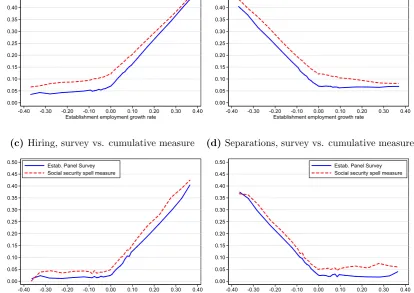
One possible explanation for the difference between our findings and those for France is that we are using six-monthly recall data from a survey, rather than changes in establishment identifiers between two years. We would naturally expect lower churning rates in data recorded between two points closer together, and we might also suspect that recall bias might have an effect. In Figure 2 we therefore compare the relationship between job and worker turnover from the survey and administrative data.

(a)Hiring, survey vs. point-in-time annual mea-sure

0.00 0.05 0.10 0.15 0.20 0.25 0.30 0.35 0.40 0.45 0.50

-0.40 -0.30 -0.20 -0.10 0.00 0.10 0.20 0.30 0.40 Establishment employment growth rate

Estab. Panel Survey Social security annual measure

(b) Separation, survey vs. point-in-time annual measure

0.00 0.05 0.10 0.15 0.20 0.25 0.30 0.35 0.40 0.45 0.50

-0.40 -0.30 -0.20 -0.10 0.00 0.10 0.20 0.30 0.40 Establishment employment growth rate

Estab. Panel Survey Social security annual measure

(c) Hiring, survey vs. cumulative measure

0.00 0.05 0.10 0.15 0.20 0.25 0.30 0.35 0.40 0.45 0.50

-0.40 -0.30 -0.20 -0.10 0.00 0.10 0.20 0.30 0.40 Establishment employment growth rate

Estab. Panel Survey Social security spell measure

(d) Separations, survey vs. cumulative measure

0.00 0.05 0.10 0.15 0.20 0.25 0.30 0.35 0.40 0.45 0.50

-0.40 -0.30 -0.20 -0.10 0.00 0.10 0.20 0.30 0.40 Establishment employment growth rate

Estab. Panel Survey Social security spell measure

in excess of employment growth) when measured from both types of social security data (point in time and cumulative), but the key feature remains: separations increase quickly in in response to employment falls. There is some evidence in Panel (a) of Figure 2 of hiring reductions, but the separation response is much larger. In short, both the survey data and the social security data suggest that the relationship between worker turnover and employment growth is similar in German and U.S. establishments.

To quantify the extent to which changes in hires contributes to changes in employment, it is convenient to estimate a piecewise linear-spline variant of (4)

hit =αhi + G

X

g=1

δ_gh(∆nitD g

it) +γ

h

t +

h

it (6)

In this specification,δh

g is the proportion of the employment change accounted for

by a change in hiring within employment growth bin g. This model is similar to that used by Albæk and Sørensen (1998), except that it uses a more flexible linear spline rather than imposing a quadratic relationship. This is more appropriate because the theoretical prediction is that there will be a “kink” in the hiring reduction at the point where employment falls exceed ¯q. If establishments reduced employment entirely along the hiring margin rather than the separation margin, then we would find δh _{= 1 for falls in employment which are smaller than ¯q (the}

quit rate). Becauseδh

g is estimated separately for each employment growth bing,

the model allows for the contribution of the hiring margin to vary in an unrestricted way.

We stress that equation (6) is only descriptive; it does not attempt to identify the causal relationship between job-turnover and worker-turnover. For example, in the model of Faberman (2008) a firm may find it optimal to continue an existing job match, but may nevertheless choose not to replace a worker who quits because of the cost of recruitment. Firms may also temporarily shrink if it takes time to find replacement hires. Thus, some firms may contract as a result of worker quits. Instead, this model allows us to examine and test in a parsimonious way whether the margin of employment adjustment varies systematically between different types of establishment and different time periods.

employment changes, in contrast, almost the entire increase is accounted for by increases in hires, indicating that establishments which grow do not reduce sep-arations, but rely almost entirely on the hiring margin. What is striking about Figure3 is that, even for very small falls in employment, the role of hiring reduc-tions is considerably less than 0.5 and falls quickly. As was clear from Figure 1, separations increase sharply when employment falls, and hence the contribution of hiring reductions is limited.

(a)Employment reductions

0.00 0.05 0.10 0.15 0.20 0.25 0.30 0.35 0.40 0.45 0.50 0.55 0.60

-0.40 -0.35 -0.30 -0.25 -0.20 -0.15 -0.10 -0.05 0.00 Employment growth rate

(b)Employment increases

0.50 0.55 0.60 0.65 0.70 0.75 0.80 0.85 0.90 0.95 1.00

0.00 0.05 0.10 0.15 0.20 0.25 0.30 0.35 0.40 Employment growth rate

Figure 3: Estimates of δ_gh from Equation (6). δ_gh measures the proportion of employ-ment change in bin g accounted for by changes in hiring. Vertical bars indicate 95% confidence intervals based on standard errors clustered at the establishment level.

How robust is this finding? In Table2we report our estimates of Equation (6) for the full sample of establishments, and test whether the basic finding holds under different assumptions and different sources of data. Our focus is on small falls in employment, so for brevity in Table 2 we report estimates of δh

g for those

values of g where 0>∆n≥ −0.2.

Row (1) reports our baseline estimate from the establishment survey. For employment falls of less than 5%, reductions in hiring account for 22% of the fall, so the remaining 78% is accounted for by an increase in separations. The proportion of the employment change accounted for by hiring reductions naturally falls for larger employment reductions, since it becomes more difficult for establishments to accommodate these falls without increasing separations.

In row (2) we use the cross-section weights which ensure that the distribution of employment in the establishment survey is representative of the distribution of employment in the population as a whole. As noted in Section 4, the survey is heavily weighted towards large establishments. If the separation responseδh_varies

Table 2: Estimates from Equation (6) with establishment and year fixed-effects. For example, δh_−0.05 is the estimated proportion of employment reduction accounted for by a reduction in hiring for 0>∆n≥ −0.05. Standard errors in parentheses are clustered at the establishment level. Job flows and worker flows are measured over the first six months of each calendar year, with the exception of the point-in-time annual measures reported in rows (3), (4) and (6).

δh

−0.05 δh−0.1 δ−h0.15 δ−h0.2 N R2

(1) IAB establishment survey (6-month) 0.207 0.116 0.100 0.069 212,673 0.742 (0.012) (0.008) (0.007) (0.007)

(2) Weighted by sampling weights 0.199 0.110 0.084 0.078 210,778 0.723 (0.027) (0.016) (0.015) (0.012)

(3) Social security annual point-in- 0.334 0.273 0.230 0.191 113,716 0.616

time measure (0.025) (0.013) (0.010) (0.009)

(4) Social security annual measure 0.389 0.312 0.270 0.230 90,759 0.663 all workers, 1999 onwards (0.034) (0.017) (0.013) (0.012)

(5) Social security cumulative measure 0.290 0.152 0.059 0.049 14,316 0.699 (0.042) (0.026) (0.023) (0.034)

(6) Social security annual point-in- 0.282 0.235 0.194 0.160 25871214 0.612 time measure (population) (0.004) (0.002) (0.001) (0.001)

(7) Excluding establishments with 0.173 0.102 0.082 0.055 157,656 0.764 vacancies att (0.014) (0.009) (0.007) (0.008)

(8) Relationship over two years 0.224 0.178 0.118 0.092 157,963 0.670 (0.021) (0.012) (0.010) (0.010)

In row (3) we estimate the same model using the social security point-in-time data (for those establishments which match to the survey data). Figure 2showed that there was substantially more churning in the social security data, and also that hires appear to fall slightly more when establishments shrink. The result is that the estimated contribution of hiring to employment reductions is larger (δh_−0.05 = 0.336), but hires still contribute significantly less than half of the total fall in employment.

In Appendix C we describe various issues in the calculation of worker flows from the social security data. In particular, we note that from 1999 onwards the social security data include records for more marginal workers (for example, those with temporary contracts). The inclusion of these workers in measures of worker flows increases the churning rate, and as a result might be expected to increase the contribution of hiring reductions to employment falls. The idea is that an estab-lishment with temporary workers which wishes to reduce employment can simply not renew contracts. Row (4) shows that the inclusion of all workers from 1999 on-wards does increase the estimate of δh

g, but does not alter our conclusion that the

In row (5) we use the cumulative measure from spell-based social security data. This makes little difference to the estimated contribution of hiring reductions. Using the entire population of establishments in row (6) also results in a similar estimate.

A potential concern is that the strong relationship between separations and small employment reductions is the result of reverse causality. Perhaps, in the short-run, establishments which lose workers via quits also shrink because it takes time to find a suitable replacement. We can investigate this possibility because the survey asks whether establishments have any unfilled vacancies. To eliminate the possibility that short-term fluctuations in employment are driven by quits, in row (7) we report estimates based on a sample of establishment which report having no vacancies. Arguably, establishments which reduce employment and which have no vacancies cannot have reduced in size because of quits. Excluding establishments with vacancies actually reduces the estimates ofδh

g. In other words,

the relationship between separations and employment reductions is stronger in these establishments.

Another similar check is provided in row (8). If short-term fluctuations in employment are caused by worker quits, then the relationship between separations and employment reductions should be less strong over a two-year interval. This does not seem to be the case, since the estimated hiring response is still small.

Overall, estimates of δh

g are quite stable across all these different samples. In

every case, the contribution of hiring reductions to even small employment falls is considerably less than one-half, confirming that German establishments which shrink do indeed increase separations, despite the institutional constraints they face.

Table 3: Estimates of Equations (6) separately by industry, establishment size, location and time periods. Standard errors in parentheses are clustered at the establishment level. Job flows and worker flows are measured over the first six months of each calendar year.

δh

−0.05 δh−0.1 δ−h0.15 δ−h0.2 N R2

Primary industries 0.160 0.093 0.090 0.078 8,645 0.806 (Agriculture, mining) (0.076) (0.055) (0.050) (0.041)

Manufacturing 0.237 0.123 0.086 0.072 67,932 0.746 (0.013) (0.009) (0.009) (0.012)

Construction 0.068 0.113 0.086 0.041 23,676 0.789 (0.052) (0.024) (0.021) (0.021)

Wholesale and retail trade 0.167 0.126 0.107 0.061 37,837 0.697 (0.024) (0.016) (0.015) (0.015)

Transport and communication 0.262 0.146 0.145 0.173 9,452 0.762 (0.059) (0.040) (0.032) (0.036)

Financial and business services 0.148 0.066 0.096 0.053 31,475 0.704 (0.049) (0.028) (0.025) (0.022)

Other services 0.266 0.112 0.128 0.087 33,656 0.735 (0.053) (0.033) (0.020) (0.020)

p-valueH0: Adjustment equal [0.002] [0.442] [0.330] [0.055]

0–10 employees 0.085 0.088 0.095 0.063 86,039 0.741 (0.158) (0.025) (0.013) (0.011)

11–20 employees 0.245 0.095 0.095 0.060 26,489 0.753 (0.048) (0.016) (0.014) (0.016)

21–30 employees 0.128 0.129 0.091 0.053 18,604 0.795 (0.030) (0.020) (0.022) (0.027)

31–50 employees 0.181 0.138 0.105 0.071 18,000 0.764 (0.036) (0.019) (0.021) (0.029)

51–100 employees 0.158 0.082 0.116 0.091 19,496 0.742 (0.030) (0.029) (0.028) (0.029)

>100 employees 0.233 0.133 0.104 0.097 44,045 0.676 (0.017) (0.014) (0.015) (0.018)

p-valueH0: Adjustment equal [0.011] [0.102] [0.944] [0.494]

Western Germany 0.220 0.128 0.106 0.079 129,181 0.713 (0.014) (0.009) (0.009) (0.010)

Eastern Germany 0.178 0.093 0.090 0.055 83,492 0.770 (0.022) (0.014) (0.012) (0.011)

p-valueH0: Adjustment equal [0.094] [0.035] [0.275] [0.123]

1993–1995 0.399 0.217 0.139 0.090 8,959 0.698 (0.044) (0.032) (0.024) (0.037)

1996–1999 0.292 0.136 0.138 0.082 25,606 0.744 (0.037) (0.023) (0.023) (0.022)

2000–2002 0.182 0.175 0.148 0.094 33,380 0.726 (0.041) (0.023) (0.021) (0.016)

2003–2006 0.177 0.092 0.086 0.029 47,542 0.781 (0.025) (0.015) (0.014) (0.018)

2007–2010 0.200 0.082 0.100 0.098 48,458 0.739 (0.029) (0.021) (0.017) (0.017)

2011–2014 0.196 0.117 0.124 0.066 48,728 0.716 (0.029) (0.022) (0.023) (0.022)

In the second panel of Table3we compare the adjustment path between estab-lishments of different sizes.6 _{The highest estimates of δ}h

−0.05 are for the two

small-est small-establishment size categories, although note that there are few observations in these categories and these estimates are rather imprecise. For establishments with more than 20 employeesδh

−0.05 increases with establishment size, although there is

no significant difference in the hiring response for larger falls in employment. But, even for the largest size category the hiring response is still only one-quarter of the total employment fall.

In the third panel of Table3we compareδh

g between establishments located in

West and East Germany.7 _{Establishments in West Germany have a significantly}

higher hiring response and therefore a smaller separation response, but the size of the difference is quantitatively small. This finding is consistent with the fact that the separation and layoff rate is higher in East Germany (see Table 1).

The final panel of Table 3 compares the adjustment path across the business cycle, using sub-periods based on the aggregate unemployment rate.8 _{If the quit}

rate is pro-cyclical, then firms which need to reduce employment in a boom will be able to shrink more easily without making layoffs and we would expect δ_gh to be pro-cyclical. However, although δh_−0.05 does vary across the periods (p-value

< 0.000), there is little evidence that it does so in a way which is systematically related to the business cycle.

Overall, our results clearly indicate that German establishments rely heavily on the separation margin when they reduce employment. The majority of any employment reduction is accommodated by increased separations, and this result is robust across establishment industry, location, size and time.

6

Why do German establishments use

separa-tions?

The key finding in this paper is that German establishments’ separation rates increase strongly when they shrink. We have shown that this result is quite robust across data sources and types of establishment. In this section we provide three pieces of evidence which help to explain this phenomenon.

6_{We use establishments’ initial size to avoid a contemporaneous relationship between size} categories and changes in employment.

7_{Establishments in West Berlin are included in the East German sample for consistency over} time.

6.1

Quits and layoffs

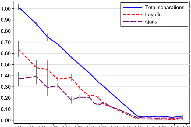
One possible explanation is that establishments allow quits rather than layoffs to accommodate falls in employment. As noted in Section2, some theoretical models predict that quit rates will increase rapidly in firms which reduce employment. In Figure 4 we plot the relationship between employment change and separations split between voluntary and involuntary separations, as defined in Section 4 (see AppendixA for a list of all separation categories).

0.00 0.10 0.20 0.30 0.40 0.50 0.60 0.70 0.80 0.90 1.00

-1.00 -0.90 -0.80 -0.70 -0.60 -0.50 -0.40 -0.30 -0.20 -0.10 0.00 0.10 0.20 0.30 0.40

Establishment employment growth rate

Total separations Layoffs

Quits

Figure 4: Relationship between layoffs, quits and job flows. We label separations as employer initiated if the respondent classified them as “Dismissal on the part of the employer”, “Leaving after termination of in-company training” or “Expiration of a temporary employment contract”. All other separations are classified as quits (see AppendixA for a list of all separation categories).

The relationship between layoffs and ∆n is stronger than the relationship be-tween quits and ∆nonly for large (>30%) falls in employment. For establishments with employment growth, quits are a larger proportion of total separations than layoffs. These patterns are similar to those observed by Davis et al. (2006, Figure 7), although in the US the point at which layoffs exceed quits occurs for smaller falls in employment. To quantify these effects more precisely, we estimate (6) but with separations as the dependent variable:

sit =αsi + G

X

g=1

δs_g(∆nitDitg) +γ s

t +

s

it. (7)

The coefficients δs

g tell us the proportion of the employment fall accounted for

negative. The first row of Table 4 reports estimates from (7) for all separations, so this replicates the base model with δs

g =δgh−1. From Table2we know that the

hiring response to a fall in employment of less than 0.05 is 0.207, so the separation response must be 0.793.

Table 4: Estimates of Equations (7) with different definitions of separation. Standard errors in parentheses are clustered at the establishment level. See Figure 4 for a def-inition of “All layoffs” and “All quits”. “Dismissals only” are defined as cause 2 and “Resignations only” are defined as cause 1 in TableA1.

γs

−0.05 γ−s0.1 γ−s0.15 γ−s0.2 γ−s0.3 γ−s0.4 N R2

(1) All separations −0.793 −0.884 −0.900 −0.931 −0.947 −0.954 212,673 0.719 (Quits + layoffs) (0.012) (0.008) (0.007) (0.007) (0.007) (0.024)

(2) All layoffs −0.352 −0.429 −0.434 −0.462 −0.456 −0.586 212,673 0.402 (0.012) (0.009) (0.009) (0.010) (0.013) (0.038)

(3) All quits −0.446 −0.454 −0.464 −0.467 −0.491 −0.362 212,673 0.304 (0.012) (0.008) (0.009) (0.010) (0.014) (0.032)

(4) Dismissals only −0.192 −0.278 −0.310 −0.340 −0.351 −0.488 212,673 0.362 (0.011) (0.008) (0.008) (0.010) (0.013) (0.038)

(5) Resignations only −0.271 −0.246 −0.251 −0.264 −0.267 −0.152 212,673 0.114 (0.009) (0.007) (0.007) (0.009) (0.012) (0.023)

In rows (2) and (3) we split total separations into those classified as quits and layoffs. As was clear from Figure 4, there is an increase in both quits and layoffs. For small falls in employment (0 >∆n ≥ −0.05) slightly more than half of all separations are classified as quits. For larger employment reductions the contribution of layoffs increases, although it is striking that quits still contribute one-third of the total employment reduction for −0.3>∆n≥ −0.4.

To some extent our classification of separations into quits and layoffs is arbi-trary.9 _{For example, cause 5 (“termination by mutual agreement” – see Appendix} A) might in fact be better thought of as a layoff. To be clear about what is driv-ing the result in Table 4, in rows (4) and (5) of we also report the relationship between job flows and those separations defined as “Dismissal on the part of the employer” and “Resignations on the part of the employee”. Here we see a larger difference in the response between the two types of separation. But, even when quits are more narrowly defined, they still account for about one-quarter of the employment reduction for small falls in employment and about one-sixth for larger falls in employment. Narrowly-defined layoffs only account for one-fifth of small falls in employment, but nearly half of large falls in employment.

Table 4 thus shows that part of the explanation for the fact that separations increase rapidly with employment falls is that the quit rate also increases rapidly.

(Recall that in the basic theoretical framework ¯q was constant.) German estab-lishments can reduce employment via separations because a substantial fraction of those separations are classified as “voluntary”. Thus, employment reductions are managed by workers choosing to leave shrinking establishments because shrinking establishments offer worse opportunities.10 _{Thus quits, or voluntary redundancies,}

an important margin which firms can use to meet reduced labour demand.

6.2

Churning and the attrition channel

The explained in Section 2, the extent to which firms can use attrition to reduce employment depends on how much worker churning there is. The higher is the quit rate at ∆n = 0, the greater the scope for reducing employment without making layoffs. To illustrate the importance of churning in allowing for attrition, we estimate ∆h

g from (6) separately for establishments grouped according to their

churning rate. For each establishment we compute the churning rate for the three previous years and separate into low (below the median), medium (median to 75th percentile) and high (above 75th percentile) churning establishments. Results are reported in Figure 5.

Churning >p75

Churning p50-p75

Churning <p50

0.00 0.05 0.10 0.15 0.20 0.25 0.30 0.35 0.40

-0.40 -0.35 -0.30 -0.25 -0.20 -0.15 -0.10 -0.05 0.00 Employment growth rate

Figure 5: Proportion of employment reduction account for by falls in hiring, establishment survey. Churning is calculated as the average of

h+s−(∆n) for periodst−1,t−2 andt−3, so the first three periods of data are lost for each establishment.

We find that δ_gh is higher for establishments with higher churning. However, even for high churning establishments we do not observe anywhere near the rates

of hiring reduction predicted by a model in which establishments use the attrition channel wherever possible. It is clear that, even for high-churn establishments, separations are an essential part of employment reduction.

6.3

Job and worker heterogeneity

The prediction that establishments should rely on the attrition channel relies on the assumption that jobs and workers within the establishment are homogeneous. In this case, workers who quit can be used to achieve the new level of employment. However, if the establishment comprises many different jobs, workers whose jobs are destroyed cannot be re-allocated to the positions of those workers who quit.11

Thus, even when an establishment is shrinking it must still make replacement hires because these jobs are still required.

The social security data allows us to test this by examining the pattern of hires and separations within narrowly defined occupations within the establish-ment. The social security data contains 369 three-digit occupation codes.12 Mean establishment employment is 147, while mean employment within an occupation within an establishment is just 11. It seems plausible therefore that jobs and work-ers within occupations are much more homogeneous than within establishments. We create a panel of occupations within establishments, and calculate the same decomposition i.e. ∆Nijt = Hijt −Sijt, where i indexes establishment as before

and j indexes occupation.

As noted in Section2, churning may be driven by workers joining and leaving a given set of jobs, or by changes in the composition of jobs. For example, an establishment may destroy a job in occupation a and create a job in occupation

b. Our occupation-establishment level panel allows us to calculate the extent to which churning is driven by the former or the latter. In Figure 6 we plot the coefficients from a fixed-effects regression of the churning rate on the employment growth rate.

Figure 6 shows that churning is indeed much lower at the occupation-estab-lishment level. At zero employment growth, more than 40% of the estaboccupation-estab-lishment- establishment-level churning is the result of changes in occupational composition within the establishment. If workers cannot easily be reallocated across occupations (as we have shown) then this provides an explanation for the continued hiring behaviour

11_{Albæk and Sørensen (1998) make exactly this point: “. . . most workers are specialised and} not easily reshuffled from vanishing jobs to jobs of otherwise separating workers”, although they do not provide direct evidence of this.

12_{The occupational classification used is theKlassifizierung der Berufe, Ausgabe 1992 (KldB}

BS aggregated at establishment level

BS aggregated at establishment-occupation level

0.00 0.02 0.04 0.06 0.08 0.10 0.12 0.14 0.16 0.18 0.20

-0.40 -0.30 -0.20 -0.10 0.00 0.10 0.20 0.30 0.40 Employment growth rate

Figure 6: Churning at the occupation level and the establishment level as a function of employment growth, computed from the point-in-time social security data (BS). Churn-ing is defined ashijt+sijt− |∆nijt at the occupation level and hit+sit− |∆nit at the

establishment level. Vertical bars indicate 95% confidence intervals based on standard errors clustered at the establishment level.

of shrinking establishments, and the fact that there is such a strong separation response. Essentially, an establishment which wishes to reduce employment in one occupation cannot use attrition from another occupation to achieve that reduction.

7

Conclusions

In this paper we use survey and administrative data to examine the relationship between employment growth and worker flows at the establishment level. This relationship is potentially a key explanation for differences in unemployment re-sponses to aggregate shocks.

administrative data and across different types of establishment.

Why do German establishments need to make use of increased separations when they reduce employment? We propose three explanations. First, a large fraction of separations, particularly for small employment reductions, are classi-fied as voluntary by establishments. Quits account for the majority of separations for employment reductions of up to 30%. Second, the level of churning in Ger-man establishments is low, and so the scope for reduced hiring is limited. Third, the heterogeneity of jobs within establishments prevent “reshuffling” of existing workers into those positions which are made vacant by attrition.

Our results are consistent with the finding (e.g. Bassanini, 2010) that both job and worker flows differ substantially across countries, and that job flows are strong predictors of worker flows. If the adjustment function is quite stable across countries, then the number of hires and separations will be driven largely by em-ployment adjustments at the firm level.

References

Abowd, J., Corbel, P. and Kramarz, F. (1999), “The entry and exit of workers and the growth of employment: an analysis of French establishments”, The Review

of Economics and Statistics 81(2), 170–187.

Abowd, J. M. and Kramarz, F. (2003), “The costs of hiring and separations”,

Labour Economics 10(5), 499 – 530.

Albæk, K. and Sørensen (1998), “Worker flows and job flows in Danish manufac-turing”, Economic Journal 108, 1750–1771.

Alda, H., Allaart, P. and Bellmann, L. (2005), “Churning and institutions: Dutch and German establishments compared with micro-level data”, IAB Discussion Paper 12/2005.

Anderson, P. and Meyer, B. (1994), “The extent and consequences of job turnover”,

Brookings Papers: Microeconomics 1994, 177–248.

Bachmann, R., Bayer, C., Seth, S. and Wellschmied, F. (2013), “Cyclicality of job and worker flows: New data and a new set of stylized facts”, IZA Discussion Paper 7192.

Bassanini, A. (2010), “Inside the perpetual-motion machine: cross-country compa-rable evidence on job and worker flows at the industry and firm level”, Industrial

and Corporate Change 19(6), 2097–2134.

Bauer, T. and Bender, S. (2004), “Technological change, organizational change and job turnover”, Labour Economics 11(3), 265–291.

Bauer, T., Bender, S. and Bonin, H. (2007), “Dismissal protection and worker flows in small establishments”, Economica 74, 804–821.

Bender, S., Haas, A. and Klose, C. (2000), “The IAB employment subsample 1975–1999”, Schmollers Jahrbuch 120(4), 649–662.

Burgess, S., Lane, J. and Stevens, D. (2001), “Churning dynamics: an analysis of hires and separations at the employer level”, Labour Economics 8, 1–14.

Centeno, M., Machado, C. and Novo, A. (2009), “Excess turnover and employment growth: firm and match heterogeneity”, IZA Discussion Paper 4586.

Cooper, R., Haltiwanger, J. and Willis, J. L. (2007), “Search frictions: Match-ing aggregate and establishment observations”, Journal of Monetary Economics

Davis, S., Faberman, R. J. and Haltiwanger, J. (2006), “The flow approach to labor markets: new data sources and micro-macro links”, Journal of Economic

Perspectives 20(3), 3–26.

Davis, S. and Haltiwanger, J. (1999), “Gross job flows”, in O. Ashenfelter and D. Card, eds, Handbook of Labor Economics, Vol. 3, Elsevier Science, 2711– 2805.

Davis, S. J., Faberman, R. J. and Haltiwanger, J. (2012), “Labor market flows in the cross section and over time”,Journal of Monetary Economics 59(1), 1 – 18. Faberman, R. (2008), “Job flows, jobless recoveries and the great moderation”, Federal Reserve Bank of Philadelphia Research Department Working Paper 08-11.

Faberman, R. J. and Nagyp´al, E. (2008), “Quits, worker recuitment and firm growth: theory and evidence”, Federal Reserve Bank of Philadelphia Working Paper 08-13.

Fischer, G., Janik, F., M¨uller, D. and Schmucker, A. (2009), “The IAB Establish-ment Panel — things users should know”,Schmollers Jahrbuch129(1), 133–148. Jahn, E. J. (2009), “Do firms obey the law when they fire workers? social crite-ria and severance payments in germany”, International Journal of Manpower

30(7), 672–691.

McLaughlin, K. (1991), “A theory of quits and layoffs with efficient turnover”,

Journal of Political Economy 99(1), 1–29.

Mortensen, D. and Pissarides, C. (1994), “Job creation and job destruction and the theory of unemployment”, Review of Economic Studies 61, 397–415.

OECD (2013), “Protecting jobs, enhancing flexibility: A new look at employment protection legislation”,in OECD Employment Outlook, Paris: OECD, chapter 2.

Appendix A

Questions used in the IAB

estab-lishment panel on worker turnover

The following questions are used to determine hires and separations:

1. Did you recruit staff in the first half of <current year>? 2. Please indicate the total number of workers recruited.

3. Did you register any staff leaving your establishment/office in the first half of <current year>?

4. Please indicate the total number of workers who left your establishment.

Respondents are also asked to distribute the total number of employees who left among 10 different categories, shown in Table A1.

Table A1: Six-month separation rate by type of separation. Table shows the mean separation rate across all establishments and all years, ¯s, the fraction of establishment-years with positive separations, Pr(sit > 0), and the average separation rate for those

establishment-years with any separations of that type, ¯s|sit>0. Weighted by sampling

weights and employment.

¯

s Pr(sit>0) (¯s|sit>0)

All separations 5.28 48.89 8.52

1. Resignation on the part of the employee 1.92 28.47 4.54

2. Dismissal on the part of the employer 1.52 22.54 4.90

3. Leaving after termination of the in-company training 0.20 6.24 1.93 4. Expiration of a temporary employment contract 0.50 11.51 2.63 5. Termination of a contract by mutual agreement 0.37 8.80 2.38 6. Transfer to another establishment within the organization 0.12 3.23 1.72 7. Retirement after reaching the stipulated pension age 0.28 11.42 1.37 8. Retirement before reaching the stipulated pensionable age 0.06 3.65 1.01

9. Occupational invalidity/ disability 0.02 1.55 0.66

Appendix B

Basic sample characteristics

Table B1: The number of establishments, average size and other key character-istics changes over the sample period, mainly due to the inclusion of additional establishments in the sample. Establishments in East Germany joined the sample in 1996.

Total no. of estab-lishments

West Germany

East Germanya

Average emp-loyment

Hiresb Separationsb

Av. no. % Av. no. %

1993 2,908 2,839 69 519 10 4.8 30 6.2

1994 2,996 2,920 76 448 13 5.1 23 12.0

1995 3,055 2,982 73 414 16 5.7 19 7.4

1996 5,785 2,935 2,850 253 8 5.9 14 8.6

1997 6,270 2,895 3,375 211 7 6.3 11 9.0

1998 6,572 2,939 3,633 197 9 6.1 8 7.9

1999 6,982 2,953 4,029 175 8 6.5 10 9.9

2000 10,402 6,094 4,308 138 7 6.1 7 7.6

2001 11,584 7,048 4,536 132 7 6.2 7 8.4

2002 11,394 7,193 4,201 126 5 5.5 6 13.1

2003 11,973 7,347 4,626 114 4 5.3 6 8.3

2004 11,839 7,321 4,518 126 4 5.2 5 7.5

2005 11,998 7,375 4,623 125 4 4.9 5 7.6

2006 11,732 7,169 4,563 116 5 5.7 5 6.9

2007 12,085 7,451 4,634 109 5 5.8 4 6.1

2008 11,986 7,250 4,736 106 6 5.7 5 6.5

2009 12,095 7,390 4,705 101 3 5.0 5 8.4

2010 12,293 7,512 4,781 93 4 5.3 4 6.8

2011 12,081 7,391 4,690 94 5 6.1 4 6.0

2012 12,133 7,407 4,726 93 5 6.0 5 6.6

2013 12,285 7,432 4,853 87 5 5.7 4 6.4

2014 12,229 7,347 4,882 83 5 6.2 4 6.7

a_{Includes West Berlin.}

0.00 0.05 0.10 0.15 0.20 0.25 0.30 0.35 0.40

Fraction of employment

-100 -50 0 50 100

% change in establishment employment

Appendix C

Calculating worker flows from the

social security data

The worker-level social security data can be used to identify when individuals join and leave establishments. However, the precise measure of hires and separations is affected by (a) the choice of which workers to include and (b) the treatment of gaps in individuals’ social security records.

Until 1999 the social security data contained information (predominantly) on permanent workers subject to social security. From 1999 onwards the data include records for other more marginal types of worker. Figure C1 shows that the hiring and separation rate is about 3.5 percentage points higher if we include all workers in the calculation as opposed to just permanent workers covered by social security. Figure C1 additionally shows that gaps in individuals’ social security record also increase the measure of hires and separations. A “gap” occurs if an individual works for establishment j in period t and at j in period t+k(k > 1) without an intervening spell of employment. If temporary layoffs are an important feature of the data, the inclusion of these gaps could make a difference. Including these gaps increases the measured hiring and separation rate by about 2.7 percentage points. In order to achieve a consistent series over the whole time period our measure of worker flows reported in the paper is based only on permanent workers covered by the social security system, and does not count a gap as a separation and hire. Note that none of these decisions changes our key conclusion as to the relationship between worker flows and job flows.

0.00 0.05 0.10 0.15 0.20 0.25 0.30 0.35 0.40 0.45 0.50

-0.40 -0.30 -0.20 -0.10 0.00 0.10 0.20 0.30 0.40

Establishment employment growth rate

Type 101, no gaps Type 101, gaps

Type 101, gaps, 99-07 All workers, gaps, 99-07