observations
.
White Rose Research Online URL for this paper:
http://eprints.whiterose.ac.uk/77830/
Version: Published Version
Article:
Salisbury, DJ, Brooks, IM and Anguelova, MD (2013) On the variability of whitecap fraction
using satellite-based observations. Journal of Geophysical Research C: Oceans, 118 (11).
6201 - 6222. ISSN 0148-0227
https://doi.org/10.1002/2013JC008797
[email protected] https://eprints.whiterose.ac.uk/ Reuse
Unless indicated otherwise, fulltext items are protected by copyright with all rights reserved. The copyright exception in section 29 of the Copyright, Designs and Patents Act 1988 allows the making of a single copy solely for the purpose of non-commercial research or private study within the limits of fair dealing. The publisher or other rights-holder may allow further reproduction and re-use of this version - refer to the White Rose Research Online record for this item. Where records identify the publisher as the copyright holder, users can verify any specific terms of use on the publisher’s website.
Takedown
If you consider content in White Rose Research Online to be in breach of UK law, please notify us by
On the variability of whitecap fraction using satellite-based
observations
Dominic J. Salisbury,1Magdalena D. Anguelova,2and Ian M. Brooks1
Received 29 January 2013; revised 9 October 2013; accepted 11 October 2013.
[1] Despite decades of effort to accurately quantify whitecap fractionWusing in situ
photography of the ocean surface, there remains significant scatter in estimates for any given 10 m wind speed (U10). It is believed that the resulting, commonly used,W(U10)
parameterizations do not fully account for the true variability inW, by failing to incorporate the impact of the wavefield and other environmental conditions. This paper attests to the variability in whitecap fraction attributed to these additional factors, by analyzing satellite-derivedWestimates over the globe for a full year. A comparison is made between the wind speed dependence of satellite estimates and threeW(U10) relationships formulated from in
situ photographic data. The influence of various secondary factors onWis investigated once the dominant wind speed dependence is accounted for. TheWretrieval’s sensitivity to secondary forcings is dependent upon microwave frequency ; at 37 GHz it varies by up to 25% of the mean at a given wind speed, while at 10 GHz it is a maximum of 8%. This results from a frequency-dependent sensitivity to foam depth ; at 10 GHz predominantly foam from active breaking waves is detected, while at 37 GHz thin foam in residual whitecaps is also seen. Principal component analysis is used to rank variables by their success in accounting for variability inW. After wind speed, the most important secondary factor that accounts for variability inWis the wavefield. A wind-wave Reynolds number accounts for almost as much variability inWas wind speed.
Citation : Salisbury, D. J., M. D. Anguelova, and I. M. Brooks (2013), On the variability of whitecap fraction using satellite-based observations,J. Geophys. Res. Oceans,118, doi:10.1002/2013JC008797.
1. Introduction
[2] Oceanic whitecaps are an important but still poorly
understood feature of the wind-driven sea [Massel, 2007]. Whitecaps form when breaking waves entrain air into the seawater forming clouds of bubbles, which subsequently rise to the surface and form patches of foam. The character-istic whiteness of sea foam is due to light scattering through the air-water mixture. The fraction of the ocean surface cov-ered in sea foam is known as the whitecap fractionW, with the global average estimated to be 1–4% [Blanchard, 1963, 1983]. Although wave breaking and whitecap formation are controlled to first order by the wind, a number of factors influence how ocean waves form, develop, break, and dissi-pate part of their energy through formation of whitecaps.
[3] A variety of physical and chemical processes are
affected by breaking waves and whitecaps at the air-sea interface, including the exchange of momentum and heat
[Andreas and Monahan, 2000 ;Fairall et al., 2003]. Bubble entrainment by breaking waves provides an efficient mech-anism for the exchange of gases, thus enhancing the total air-sea transfer [Woolf, 1997 ; Wanninkhof et al., 2009] ; it has been argued that the bubble-mediated contribution should scale withW[Monahan and Spillane, 1984 ;Woolf, 2005]. Whitecaps are areas where sea spray droplets are actively produced through bubble bursting, and via the wind tearing of wave crests at higher wind speeds [ Blan-chard, 1963; Monahan et al., 1983 ; Andreas, 1995]. Recently, the importance of wave breaking and whitecap formation in the transfer of organic matter from the ocean surface into the atmosphere has been increasingly recog-nized [e.g., Monahan and Dam, 2001 ; O’Dowd et al., 2004, 2008; Vignati et al., 2010; de Leeuw et al., 2011]. Upon injection into the lower atmosphere, spray droplets can play a variety of roles depending upon their size. Smaller droplets (r1 lm), having a residence times of
the order of days, play a vital role in the climate system both directly through the scattering of solar radiation [ Hay-wood et al., 1999], and indirectly by acting as cloud con-densation nuclei, and thus affecting cloud albedo [Andreae and Rosenfeld, 2008]. Larger droplets (r25lm), despite
having short residence times of the order of seconds, can affect interfacial fluxes of sensible and latent heat at high wind speeds [Andreas et al., 1995, 2008], and are believed to affect the intensity of tropical cyclones [Andreas and Emanuel, 2001].
1Institute for Climate and Atmospheric Science, University of Leeds,
Leeds, UK.
2Remote Sensing Division, Naval Research Laboratory, Washington,
District of Columbia, USA.
Corresponding author: D. J. Salisbury, Institute for Climate and Atmos-pheric Science, University of Leeds, West Yorkshire, Leeds LS2 9JT, UK. ([email protected])
VC2013. American Geophysical Union. All Rights Reserved.
[4] The presence of whitecaps increases ocean albedo
[Koepke, 1984] and thus must be accounted for in models of the global radiation budget [Frouin et al., 2001]. Consid-eration of whitecaps is also required in optical ocean color retrievals due to the masking of water-leaving radiance by foam patches [Gordon and Wang, 1994]. At microwave frequencies, whitecaps are areas with increased surface emission and brightness temperature [Wentz, 1983;Smith, 1988 ; Rose et al., 2002]. This has implications for many remote sensing applications, including the use of satellite-borne radiometers to obtain the surface wind vector [Wentz, 1997 ;Yueh, 1997 ;Gaiser et al., 2004].
[5] An accurate parameterization of whitecap fraction is a
requirement for successful modeling of whitecap-dependent processes. In nearly all current geophysical models, whitecap fraction is specified as a simple function of wind speed, W(U10), where U10 is the wind speed at a 10 m reference
height. As such, a reliable estimate ofWis only obtained if it is assumed that wind speed can fully predict whitecap frac-tion; however, there is substantial evidence that this is not the case [Monahan and O’Muircheartaigh, 1986;Anguelova and Webster, 2006;Callaghan et al., 2008b].
[6] Here we present an analysis of the variability of
whitecap fraction using satellite-derived estimates ofW. In section 2, we summarize relevant background information and outline the need for a comprehensive database of W measurements in the light of the limitations of using in situ data. Section 3 describes the data used in this study, the cal-culation of additional factors influencing whitecap fraction, and the analyses used. In section 4, we explore the wind speed dependence of satellite-derived W, investigate the dependence of W on various factors, and quantify how important each variable is in accounting for variability in W. We follow with a discussion of our findings (section 5), and conclusions (section 6), regarding the variability of whitecap fraction and the utility of satellite-derived esti-mates ofWfor future direct monitoring and quantifying of this variability.
2. Whitecap Observations
2.1. Traditional Measurement of Whitecap Fraction
[7] Estimates of whitecap fraction have traditionally
been obtained from in situ measurement of the ocean sur-face via photographic or video imagery [Lewis and Schwartz, 2004; Anguelova and Webster, 2006 ; de Leeuw et al., 2011]. Measurements have been made from aircraft [e.g., Bobak et al., 2011 ;Kleiss and Melville, 2011], ships [e.g., Callaghan et al., 2008a], and fixed platforms [e.g., Callaghan et al., 2008b ;Sugihara et al., 2007].Anguelova and Webster [2006] give a chronological listing of white-cap fraction data sets spanning nearly 50 years, from 1952 to 2000. There exists large variation in estimates of white-cap fraction, spanning several orders of magnitude. Part of this variation is likely due to differences in both whitecap observation methods and wind speed measurement meth-ods. Furthermore, conditions encountered between differ-ent measuremdiffer-ent campaigns also show large variation, yet often there is not sufficient documentation of environmen-tal conditions (such as sea surface temperature, air-sea sta-bility, and wave state) to make a reliable comparison between data sets.
2.2. Previous Wind Speed Parameterizations of Whitecap Fraction
[8] Wind speed is the first-order controlling factor for
wave breaking and the formation of whitecaps, and being routinely measured, is often used to parameterize whitecap fraction through an empirical expression, W5f(U10).
Nearly all of these relationships are expressed as a power law of the formaUb
10 with the exponentbtypically close to
three [Anguelova and Webster, 2006]. A cubic relationship betweenWand a wind parameter (either wind speed or fric-tion velocity, u*) has a strong theoretical grounding: Car-done [1969] hypothesized that W, related to energy dissipation through wave breaking, should be directly related to the rate of energy transferred to the wavefield through the action of the wind. Wu[1988] determined this on dimensional grounds by noting thatWshould be propor-tional to the energy flux supplied by the wind, which is itself proportional to the cube of the turbulent friction velocity.
[9] As numerous parameterizations exist within the
litera-ture, it is often a matter of preference as to which formulation should be utilized. Despite being one of the earliest formula-tions, the Monahan and O’Muircheartaigh [1980] relation-ship, obtained using the robust biweight fitting technique on a combination of field data reported in Monahan [1971] and Toba and Chaen [1973], has been widely adopted in the parameterization of sea spray aerosol production in models:
WðU10Þ53:8431024U103:41; (1)
whereW is in %. The highest wind speed recorded in the combined data set is 16.6 m s21
, but a maximum wind speed above which (1) is no longer suitable, is not explic-itly defined.
[10] The Callaghan et al. [2008a] relationship is a recent
formulation resulting from analysis of whitecap data obtained during the 2006 Marine Aerosol Production (MAP) campaign in the North East Atlantic. By assuming thatWcan be related toU10with a power law of the form W5aðU101bÞ3, a linear regression on W1/3 against U10
was performed, resulting in the following relationships :
WðU10Þ53:1831023ðU1023:70Þ3; 3:70<U1011:25; WðU10Þ54:8231024ðU1011:98Þ3; 9:25<U1023:09;
(2)
whereWis percentage total whitecap cover. Note that data have been divided into two overlapping groups according to the measured wind speed, with a regression performed on each group.
[11] In the study ofGoddijn-Murphy et al. [2011], analysis
of the MAP whitecap data set was extended through use of in situ, model, and satellite data for wind and waves. The following W(U10) relationship is reported when NASA
QuikSCAT satellite wind speed measurements are used :
WðU10Þ511:531023U101:86: (3)
2.3. Known Variability of In Situ Whitecap Fraction Observations
[12] The pooling of many historical data sets has
wind speed [Anguelova and Webster, 2006]. Part of this variability is likely due to the use of different measurement techniques ; this is especially true of earlier data sets where data volume is generally much lower, and measurement techniques less consistent. It has been shown byCallaghan and White[2009] that to obtain an individual estimate ofW with a fractional error of a few percent, one needs to aver-age over hundreds of individual photographs (or video frames) within an interval short enough to have constant forcing. Analysis of an insufficient number of images—as was the case in many of the earlier studies—can lead to nonconvergent W estimates with larger uncertainties, con-tributing to data scatter [Callaghan and White, 2009].
[13] More recent data sets [Lafon et al., 2007 ;Sugihara
et al., 2007;Callaghan et al., 2008b] show a clustering of W estimates when plotted as a function of U10[de Leeuw et al., 2011]. This clustering is indicative of improvements to the extraction ofWfrom photographic data and increases in data volume, although it should be acknowledged that the clustering may in part be due to the similar image proc-essing methodology adopted in these recent studies.
[14] The almost order-of-magnitude scatter that remains
is likely an indication that factors other than wind speed play a role in determining whitecap fraction. We discuss these factors below (sections 2.3.2 and 2.3.3), but first we consider how variability inWmay in part be a consequence of the sensitivity ofWestimates to measurement of differ-ent stages of whitecap lifetime.
2.3.1. Active and Residual Whitecaps
[15] Although individual whitecaps are in constant
tem-poral evolution, it is possible to define two distinct phases of a whitecap’s life-cycle [Monahan and Lu, 1990]. During the active breaking stage, air is entrained into the water col-umn at the wave crest, with associated generation of under-water noise due to bubble formation and fragmentation [Deane and Stokes, 2002; Callaghan et al., 2013]. As the leading wave crest progresses forward, it continues to entrain air. The resulting surface expression is a dense layer of foam with a visible albedo of around 0.5 [Whitlock et al., 1982], termed active (or stage A) whitecaps.
[16] Following active air-entrainment, the whitecap enters
its second phase (stage B) as bubbles in the subsurface plume rise to the surface due to buoyancy and turbulent forces. Once at the surface, the lifetime of risen bubbles is dictated by a combination of seawater chemistry (e.g., salinity, satu-ration levels of dissolved gases), turbulent forces, thin film fluid drainage, and stabilizing or destabilizing forces [ Calla-ghan, 2013]. The gradually decaying surface foam layer per-sists as long as there is a sufficient flux of bubbles to the surface. While subsurface and surface parts of the whitecaps are closely related, the surface foam layers are the subject of interest for microwave remote sensing, excluding deeper bubble plumes [Anguelova and Gaiser, 2011].
[17] Whilst many authors have aimed to report
measure-ments of active or residual whitecaps only, the task of sepa-rating these signals in photographic data is not straight forward. Furthermore, it is probable that due to the lack of consistency between different measurement techniques used, estimates ofWfrom an individual data set are some-what conditional on the measurement technique.
[18] Callaghan et al. [2012] suggest that much of the
scatter between whitecap fraction estimates from different
data sets could be due to the variability in foam decay times between different observations. Such variability can signifi-cantly affect estimates of residual whitecap fraction, which is known to dominate measurements of totalW [Monahan and Lu, 1990;Callaghan et al., 2012]. It has been shown that factors such as the scale (or intensity) of breaking waves [Jessup et al., 1997; Callaghan et al., 2012], sea surface temperature [Bortkovskii and Novak, 1993], salinity [Monahan and Zietlow, 1969 ; Peltzer and Griffin, 1987], and surfactant concentration [Callaghan et al., 2012, 2013], can influence the lifetime of foam layers. It is there-fore possible that a large degree of variability inWmay be attributed to these effects (see section 2.3.3).
[19] The remote sensing signature of foam layers at
dif-ferent frequencies has been related to characteristics of the foam layer, specifically the foam layer thickness [ Angue-lova and Gaiser, 2011]. With satellite estimates ofW, it is possible to differentiate between foam of different thick-nesses, and thus make some distinction between active and residual whitecaps (section 3.1.2).
2.3.2. Influence of the Wavefield
[20] Over recent years, there has been increased focus on
the effect of the wavefield on W. Several recent whitecap data sets include an assessment of how the wavefield may affect W, often through classifying W measurements by a measure of the degree of wave development, and then fit-ting aW(U10) curve for each class.
[21] Stramska and Petelski [2003], working with data
obtained in the North Atlantic, categorized measurements of W by the corresponding wave conditions; this was achieved by comparing measured significant wave height, Hs, with that expected for a fully developed sea [Pierson et al., 1955]. They concluded that at a given wind speed, a developed sea should result in a slightly higher whitecap fraction than that of an undeveloped sea, suggesting that the wind duration or fetch is an important factor in deter-miningW.
[22] Sugihara et al. [2007] found evidence that
white-caps are produced most actively under the condition of a pure wind sea, and that W is suppressed by swell. The authors find that in conditions of a pure wind sea, at a given value of U10, W increases with wave age, supporting the
conclusions ofStramska and Petelski[2003]. In contrast to the above two studies, Lafon et al. [2007]—by analyzing photographs taken in a coastal environment—found that there is a peak inWat an intermediate wave age, and that Wis likely to be lower both above and below this point.
[23] Callaghan et al. [2008b], focusing on a
fetch-limited coastal region, observed that : (i) scatter in W was reduced when seas were mixed (i.e., when the spectral intensity of wind waves is of the same order of magnitude as the swell) rather than dominated, (ii) swell-dominated seas result in overall lower values of W than mixed seas (as inSugihara et al. [2007]), and (iii) the pres-ence of a tidal current can augmentWestimates under cer-tain conditions.
[24] Most recently, Goddijn-Murphy et al. [2011]
pro-vided evidence that, at a given wind speed for higher winds (U10>10 m s21), W is slightly larger in conditions of
had previously come to the same conclusion, reporting higher values ofWin cases of decreasing winds (developed seas). Goddijn-Murphy et al. [2011] also concluded that whitecap fraction is generally reduced in swell-dominated conditions compared to wind sea conditions in cases of cross swell (angle between direction of wind and swell waves between645and6135).
[25] In evaluating the effect of the wavefield onW, it can
prove difficult to isolate the effect of the wavefield because of inherent correlations between wind speed and measures of the degree of wave development. Many different meas-ures of sea state have been adopted ; these vary in how exactly the degree of wave development should be defined in terms of readily available measurements. BothStramska and Petelski[2003] andSugihara et al. [2007] consider the effect of wave development onW; however, the classifica-tion ofStramska and Petelski[2003] is based on significant wave height only, which may include contributions from swell, while Sugihara et al. [2007] used directional fre-quency wave spectra to separate swell-dominated from pure wind seas. This makes a direct comparison of their results questionable.
[26] On a practical level, individual in situ data sets are
likely to span only a narrow range of possible wave condi-tions due to the temporal and spatial limitacondi-tions of an indi-vidual field campaign, so that a direct comparison of results between studies may not be viable.
2.3.3. Influence of Other Environmental Factors
[27] It has proven difficult to quantify the dependence of
W on sea surface temperature (SST). Only a handful of studies of whitecap fraction consider this effect ; further-more, where data for SST does exist, conditions are often limited to a small range of temperatures.
[28] Both Monahan and O’Muircheartaigh [1986] and
Spillane et al. [1986] found evidence that increasing SST can increase the exponent in a W-U10 power-law fit, but
with no overall increase inW. Monahan and O’Muirchear-taigh [1986] reason that the true cause of such a result is the inherent correlation between SST and average duration of high wind events ; at higher latitudes (lower SSTs), the average duration of these events is shorter, leading to a wave spectrum that is not fully developed. It is worth not-ing that these results rely on a comparison of multiple dif-ferent data sets obtained at difdif-ferent SSTs. Given the different ranges of other conditions encountered by the var-ious studies, the conclusions must be treated with some caution.
[29] Bortkovskii and Novak [1993] compiled a much
larger data set, including both their own measurements in a range of water temperatures, and those of other research groups. They found that the rate of wave breaking increased with increasing SST, but that the lifetime of the resulting foam patch decreased. The net result on total whitecap fraction is unclear.
[30] Both Monahan and O’Muircheartaigh [1986] and
Bortkovskii and Novak [1993] ascribe the temperature dependence of wave breaking to the associated changes in viscosity.Monahan and O’Muircheartaigh[1986] hypothe-size that as viscosity decreases (increasing SST) there is less viscous dissipation in waves, and hence more energy available for wave breaking. They also note that with lower water viscosity the bubble size distribution shifts to smaller
bubbles [Pounder, 1986], which have lower terminal veloc-ities, resulting in increased foam lifetime and thus higher W. Wu [1988] and Stramska and Petelski[2003] reported no systematic trends in W with SST. In summary, whilst SST can alterWthrough several different mechanisms, its overall effect onWis not yet clear.
[31] Atmospheric stability is thought to affectWthrough
its influence on the surface momentum flux. The air-sea temperature difference DT5Ta2Ts is often used as a proxy for atmospheric stability—a negative DTrepresents unstable conditions, a positiveDTstable.
[32] Monahan and O’Muircheartaigh [1986] find
evi-dence for greater values of W under unstable conditions than stable conditions at the same wind speed, with W increasing by nearly 10% perC, at a fixed wind speed.Wu
[1988] concluded that W will increase as conditions become more unstable, based on an hypothesized relation-ship between the drag coefficient andDT. However, Stram-ska and Petelski [2003] found no evidence of a relation betweenDTandWat a given wind speed.
[33] Monahan and Woolf [1988] quantified the stability
effect on active and residual whitecap fractions separately. Estimates using their empirical expressions show that the largest changes resulting from stability effects would be on stage A whitecaps with an increase of a factor of 7 from neutral to unstable conditions with DT5 210C ; the increase in stage B whitecap fraction would be a factor of 2.4.
[34] Again, there is no general consensus as to the effects
of atmospheric stability onW; those trends that have been observed are small relative to the spread of data.
[35] Whilst the salinity difference between freshwater
and saltwater can have a large effect on the persistence of bubble plumes, and thusW [Monahan and Zietlow, 1969], the effect is expected to be much more subtle over the rela-tively small range of salinity variations encountered in the open oceans. Peltzer and Griffin[1987] demonstrated that changes to foam lifetime due to salinity are insignificant in the open ocean.
[36] The role surface-active substances (surfactants) play
in modulatingWin the open ocean has yet to be evaluated, although some laboratory studies do exist [Garrett, 1967 ; Scott, 1986 ; Peltzer and Griffin, 1987]. Recently, Calla-ghan et al. [2013] confirmed that the presence of surfac-tants acts to stabilize surface bubbles and so increase whitecap decay times. As the concentration of surfactants is known to vary markedly over the global oceans [ Falkow-ski et al., 1998;McClain et al., 2004], it is plausible that presence of such material can significantly affect residual whitecap fraction.
2.4. Need for Global Measurement of Whitecap Fraction
[37] In situ observations, while instrumental in gaining
measurements are often limited both spatially and tempo-rally, obtaining measurements in a limited range of condi-tions. Most in situ data sets have been obtained in near-coastal, fetch limited conditions, and at high latitudes with cold waters [Anguelova and Webster, 2006]; data from the open ocean and warm waters (SST>17C) are very sparse. [38] In contrast, satellite-based estimates of W can
pro-vide long term, consistent, global estimates of whitecap fraction. Furthermore, with accompanying measurements of many different variables, a thorough study of the vari-ability in whitecap fraction is now viable.
3. Methods
3.1. Satellite-Based Estimates of Whitecap Fraction 3.1.1. Passive Microwave Remote Sensing of Whitecaps
[39] Microwave radiometry is a well-developed passive
remote sensing technique that uses the natural emissivity of the ocean surface in its various states—smooth, roughened by small and large scale waves, and covered with sea foam [Ulaby et al., 1981, chap. 4]. Changes in ocean surface emissivity are observed by microwave radiometers as changes to the brightness temperature TB of the ocean surface.
[40] Anguelova and Webster [2006] demonstrated the
feasibility of estimating W from routine satellite measure-ments ofTBat 19 GHz, horizontal polarization. This initial algorithm used TB observations from the Special Sensor Microwave Imager (SSMI/I) [Wentz, 1997], a radiometer flown on satellite platforms F8 to F17 of the United States Department of Defense since 1987 and operating at four frequencies between 19 GHz and 85 GHz. The algorithm for estimating W combines satellite TB observations with models for the rough sea surface and foam-covered areas (whitecaps). An atmospheric model is used to remove the influence of the atmosphere from the satellite measured top-of-atmosphereTB, in order to obtain the changes inTB at the ocean surface. Wind speedU10, wind directionUdir,
SST at the ocean surface, and atmospheric variables such as water vapor and cloud liquid water are necessary as inputs to the atmospheric, roughness, and foam models. Although various models and many variables are involved in the algorithm estimatingW, for simplicity we denote this theW(TB) algorithm.
[41] The algorithm for estimating W has since been
improved in several respects [Anguelova et al., 2009]. Notably, more physically robust models for rough and foam-covered surfaces are now employed [Bettenhausen et al., 2006 ;Johnson, 2006 ;Anguelova and Gaiser, 2013], as are independent data sources for input variables in the W(TB) algorithm. Details on the improvedW(TB) algorithm will be given in a future paper ; below we briefly summa-rize information relevant for this study.
[42] The use of independent input data sets in theW(TB) algorithm has been possible due to newly available TB observations since 2003—in addition to those of SSM/I— from the microwave radiometric sensor WindSat, onboard the Coriolis satellite [Gaiser et al., 2004]. WindSat oper-ates at five frequencies, from 6 GHz to 37 GHz, thus pro-viding more TB data suitable for remote sensing of whitecaps than SSM/I [Anguelova and Gaiser, 2011]. The
Coriolis satellite completes 14 orbits per day, with ascend-ing (northbound Equator crossascend-ing) and descendascend-ing (south-bound Equator crossing) passes at local times of approximately 18 :00 and 06 :00, respectively. There are 80 pixels within the WindSat swath with an approximate spac-ing of 12.5 km across the swath and along the satellite track [Bettenhausen et al., 2006]. At the lowest level, each pixel within the WindSat swath represents a TB (or W) value averaged over an area of 50 km 3 71 km. Each W value resulting from such an intrinsic spatial averaging of satel-lite instantaneous samples is analogous to the temporal averaging required to produce stableWvalues from instan-taneous photographic data (section 2.3). WindSatTBdata at higher swath resolutions (i.e., pixel value averaged over an area of 35 km353 km or 25 km335 km) are also avail-able, but the work here uses whitecap fraction estimates at the low resolution.
[43] Use of TB data from WindSat in the W(TB) algo-rithm allows independent use of SSM/I data (water vapor and cloud liquid water) for the atmospheric correction. In addition, the input variables U10, Udir, and SST to the
atmospheric, roughness, and foam models in the W(TB) algorithm are also compiled from independent sources (section 3.1.3).
3.1.2. Whitecap Database
[44] Whitecap fraction estimates were obtained by
run-ning the W(TB) algorithm for all five WindSat frequencies and both horizontal and vertical polarizations at swath reso-lution. All available WindSat orbits for 2006 with both ascending and descending passes were used. A subset of this pool of raw swath data for whitecap fraction was then used to compile a more tractable database of satellite-based W estimates, accompanied by six meteorological and oceanographic variables ; hereafter we refer to this database as ‘‘W database.’’ The compilation of the W database involved three main activities : (i) devising a criterion to choose a subset of all W data ; (ii) gridding the W values from swath resolution into regular global maps ; and (iii) matching additional variables to the griddedWvalues. The following briefly describes activities (i) and (ii) ; section 3.1.4 informs on (iii).
[45] TheWdatabase consists of whitecap fraction values
whitecaps [Anguelova and Gaiser, 2011], we expect thatW estimates at 10 GHz will predominantly be representative of active, stage A (section 2.3.1), whitecaps and to some extent residual foam (stage B) when it is thicker, e.g., at higher wind speeds. At 37 GHz,Westimates will represent total whitecap cover (stages A and B).
[46] The swath W values at 10 GHz and 37 GHz were
gridded onto a 0.530.5grid. For each grid cell, an aver-age value of all swathW samples falling within the cell is calculated. These cell-averages for each frequency, here-after referred to asW10andW37, represent a mean estimate
of whitecap fraction for the cell at the local time of the sat-ellite overpass. The gridding procedure allows some useful statistics to be obtained for the swath samples contributing to a given grid cell. These include the root-mean-square (rms) error, standard deviation rW, and count (the number of individual swath samples averaged to obtain the daily meanWfor the cell).
3.1.3. Basic Additional Variables
[47] Whitecap fraction data at swath resolution are
matched in time and space with six meteorological and oceanographic variables ; wind speed U10, wind direction Udir, SST, air temperature Ta, significant wave height Hs (defined as 4 ffiffiffiffi
E
p
, whereE is total wave energy), and peak wave periodTp(defined as the period corresponding to the highest peak in the one-dimensional frequency spectrum of the wavefield). These basic additional variables are taken from independent sources.
[48] Wind vector (U10 andUdir) is taken from the
Sea-Winds microwave scatterometer on-board the QuikSCAT satellite (http ://winds.jpl.nasa.gov/missions/quikscat). The matching criterion between WindSat and SeaWinds meas-urements is within 25 km and 60 min.
[49] When a SeaWinds matchup is not available,U10and Udirfrom the model output (every 6 h) of the Global Data
Assimilation System (GDAS) of National Centers for Envi-ronmental Prediction (NCEP) is used. GDAS is the system used by the NCEP global forecast model to place myriad observations (including those of QuikSCAT) into a gridded model space for the purpose of initializing weather fore-casts with observed data (http ://www.ncdc.noaa.gov/ model-data/global-data-assimilation-system-gdas). We use GDAS outputs closest in time and spatially interpolated to the location of the WindSat data.
[50] To ensure that use of two different wind speed
sour-ces does not introduce bias, we explore the distribution of swath resolution U10 values from QuikSCAT and GDAS,
for 1 October 2006 (Figure 1a). The shapes of the probabil-ity densprobabil-ity functions for the two sources are similar.
[51] Differences of a few percent are visible at low wind
speeds (U10<5 m s21) where QuikSCAT values are higher
than those of GDAS ; GDAS values are higher forU10>11
m s21
. Note that this is not a comparison of paired QuikSCAT—GDAS values for U10 at a given location ; at
each point we have either a QuikSCAT or GDAS value. For theU10values considered in Figure 1a, we find that in
general GDAS has more counts at high latitudes and low latitudes, while in the midlatitudes, a larger count is from QuikSCAT values. It is therefore logical that GDAS gives higher probability for high winds than QuikSCAT, while QuikSCAT gives higher probability for low winds. Figure
1b shows a histogram of gridded wind speed values coupled withWdata for 2006.
[52] Data for SST andTa(at 2 m above the surface) are also from GDAS. HsandTpvalues are from NCEP Wave Watch III (WW3) model. We have used the historical archive of wave hindcast results produced with version 2.22 of WW3 at 3 h intervals (http ://polar.ncep.noaa.gov/ waves/implementations.shtml). The input variables for WW3 are from GDAS. The WW3 model also gives peak wave direction, but it is not currently included in the data-base. The temporal and spatial matching criteria for WindSat and WW3 data are as those for GDAS. Table 1 summarizes information for these variables, including their spatial resolutions, use, and access.
[53] All these variables, matched up initially to WindSat
data in swath resolution, are gridded in the same way as the W estimates (section 3.1.2). Mean daily values, as well as statistics (root-mean-square error, standard deviation, and count), are obtained for each variable for each grid cell.
3.1.4. Data Used in This Study
[54] This study makes use of the gridded satellite-based
estimates of whitecap fraction from both 10 GHz and 37 GHz, W10 andW37. Data for all of 2006 are used in daily
and monthly format. Figures 2a and 2b present daily global maps ofW10andW37along both ascending and descending
passes for 1 October 2006. The resulting spatial match is patchy because the ascending and descending passes of the Coriolis and QuikSCAT satellites are out of phase. Figures 2c and 2d show monthly maps for October 2006.
0 10 20 30
0 5 10 15 20
U
10 (m s
−1)
Probability Density (%)
(a)
QuikSCAT GDAS
0 10 20 30
0 2 4 6 8
U
10 (m s
−1)
log
10
count
[image:7.610.342.518.76.360.2](b)
Figure 1. (a) Probability density function of swath reso-lution U10 values from QuikSCAT and GDAS for 1
Table 1.Sources of Database Variables, With Resolution and Data Access
Model/Sensor (Satellite)
Access Variable (units) Grid Resolution Variable Use
Windsat (Coriolis) Naval Research Laboratory
Brightness temperatureTB(K) 0.5o30.5o W(TB) algorithm
SSM/I (F13)
Remote Sensing Systemsa
Water vapor Cloud liquid water
0.25o
30.25o W(T
B) algorithm
SeaWinds (QuikSCAT) PODAAC/JPLb
Wind speedU10(m s21)c
Wind directionUdir(o)
0.25o
30.25o W(T
B) algorithm &Wdatabase
GDAS/NCEPd
CISL RDAe
U10,Udir, SST (oC)
Air temperatureTa(oC)
1o
31o W(T
B) algorithm &Wdatabase
Wdatabase
WaveWatch III/ NOAA NCEPf
Significant wave heightHs(m) Peak wave periodTp(s)
1o
31.25o
Wdatabase
World Ocean Atlas 2005 NOAAg
Salinity—surface field 1o
31o ExpandWdatabase
a
www.remss.com.
bPhysical Oceanography Distributed Active Archive Center at the NASA Jet Propulsion Laboratory (http://podaac.jpl.nasa.gov). c
Satellite wind estimates (such as those from QuikSCAT) are calibrated to equivalent neutral wind speeds [Kara et al., 2008]. Model winds are also corrected to neutral winds.
d
Global Data Assimilation System, National Centers for Environmental Prediction (http://www.emc.ncep.noaa.gov/gmb/gdas/).
eResearch Data Archive at Computational and Information Systems Laboratory (http://rda.ucar.edu/datasets/ds083.2/). f
National Centers for Environmental Prediction (http://polar.ncep.noaa.gov/).
gNational Oceanographic Data Center (http://www.nodc.noaa.gov/OC5/WOA05/woa05data.html).
120oW 0o 120oE
60oS
0o
60oN
120oW 0o 120oE
60oS
0o
60oN
(a)
120oW 0o 120oE
60oS
0o
60oN
120oW 0o 120oE
60oS
0o
60oN
(b)
W (%)
0 1 2 3 4 5 6
120oW 0o 120oE
60oS
0o
60oN
(c)
120oW 0o 120oE
60oS
0o
60oN
(d)
W (%)
0 0.5 1 1.5 2 2.5 3 3.5
[image:8.610.68.542.375.722.2][55] Explicit calculation of the error on individual W
estimates is not currently available due to the complex mul-tivariable nature of the W(TB) algorithm. However, where applicable, we have used the statistics obtained during the gridding process to screen for unreliable W estimates resulting from, for example, a low count in a particular grid cell, or an exceptionally large variation between individual swath samples.
[56] We expect some correlation between W10 and W37
values and the basic additional variables. The reason is that the sameU10,Udir, and SST values used in theW(TB) algo-rithm at swath resolution (section 3.1.1) are also entries in theWdatabase in gridded format. We tolerate some corre-lation because we did not see substantial gains in seeking different sources forU10,Udir, and SST data. For instance,
we aim to use all availableWestimates, of which there are more than 18 million ; this would not have been possible with a more selective temporal and spatial match-up with direct measurements from other satellites or buoys. Gains in using independent data would have also been limited if we used model outputs different from those provided by GDAS (e.g., use of the European Centre for Medium-Range Weather Forecasts (ECMWF)) considering that assimilation of buoy and satellite measurements in any model is a common practice. Indeed, assimilation of the QuikSCAT data in ECMWF and NCEP have led to wind component values differing by at most 1.5 m s21
[Chelton and Freilich, 2005].
[57] We expanded our set of six basic variables in the
current whitecap database with salinityS. We use monthly mean salinity fields from the NOAA World Ocean Atlas 2005 (WOA05) (accessible online at www.nodc.noaa.gov/ OC5/WOA05/pr_woa05.html).
[58] The expansion of theWdatabase with further basic
additional variables (e.g., wave direction from WW3, cur-rents, ocean color as a proxy of surfactants) and fully inde-pendent data (e.g., wind and SST) is planned future work.
3.2. Derived Additional Forcing Variables
[59] In addition to the variables listed in Table 1 as
entries in the W database, several further parameters are constructed to assess their influence on W. Atmospheric surface layer stability is indicated by the air-sea tempera-ture difference DT5Ta2Ts. The kinematic viscosity of water, vw, is calculated using a combination of daily SST fields and monthly mean salinity fields.
[60] Two dimensionless wind-wave variables are
consid-ered. The breaking-wave Reynolds number, defined as:
RB5 u2
xpma
; (4)
where xp is the spectral peak angular frequency of wind waves, andvais the kinematic viscosity of air. The consid-eration of such a nondimensional variable as an appropriate parameter to describe wave breaking dates back to the work ofToba and Chaen[1973], withRBin its above form first suggested as a parameter to describe whitecap fraction by Toba and Koga [1986]. The roughness Reynolds number,
RHw5 uHs
mw
; (5)
is a slightly modified version of that of Zhao and Toba [2001], the only difference being the use of the kinematic viscosity of watervwinstead ofva, following the suggestion ofWoolf[2005].
3.2.1. Measures of Wave Development
[61] Recent in situ studies have strived to explicitly
evalu-ate the role of the wavefield on variability inW. Wave age
U—defined as cp/u*, where cpis the wave phase velocity and u*the air-side friction velocity—can be used to infer
the stage of development of the sea.Ucan be expressed in terms of readily available measurements as :
U5 gTp
2ppffiffiffiffifficdU10
; (6)
by usingcp5gTp=ð2pÞ[Hanley et al., 2010]. Herecdis the drag coefficient, calculated following Large and Pond [1981].
[62] We also calculate the mean wave slope MWS (also
referred to as significant steepness or simply wave slope),
MWS52pHs gT2
p
; (7)
which is a measure of the steepness of the dominant waves. Note the use of the peak wave period in this formulation (the only available wave period measure), as opposed to the mean wave period. Although it has been shown that MWSalone cannot predict whether an individual wave will break [Holthuijsen, 2007], here we consider this quantity as a bulk measure of the degree of wave development that combines the effects ofHsandTp. AsMWSis not explicitly dependent upon wind speed, it is included in our analysis of variability in W once the wind speed dependence has been accounted for (section 4.2.1). The dependence of W onMWShas not previously been considered.
3.2.2. Classification of the Wavefield
[63] A different approach to assessing the influence of the
wavefield involves categorizing W estimates by degree of wave development. Ideally, spectral wave data would be used to reveal the presence (and relative intensity) of differ-ent regimes such as wind sea and swell [e.g., Sugihara et al., 2007;Callaghan et al., 2012]. Detailed wave spectra are not available here ; however, it is possible to use the two wave measures available in the current database (Hs andTp), together withU10, to attempt a broad classification
of Westimates by the stage of wave development. A simi-lar approach was adopted in the study of Stramska and Petelski [2003], where U10 and Hs measurements were used to classify data into three groups ; those obtained in undeveloped seas, those obtained in developed seas, and those obtained under conditions of decreasing winds. They note that while this criterion is not exact, it does allow an insight into the effects that sea state can have onW.
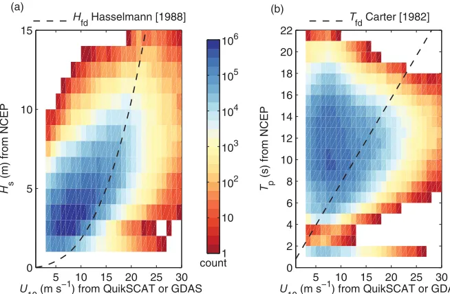
[64] Classification by significant wave height is as
fol-lows. At each individual grid cell, the recorded value ofHs is compared with Hfd, the significant wave height that
equilibrium with the wind.Hfdis calculated from the
wind-wave relation in the WAM model [Hasselmann et al., 1988],
Hfd51:61431022U102; 0<U107:5;
Hfd51022U10218:13431024U103; 7:5<U1050:
(8)
This relationship defines the sea state as eitherswellwhen Hs>Hfdorwind seawhenHs<Hfd. At the threshold level,
where Hs5Hfd, it is assumed that the seas have just
become fully developed.
[65] Similarly,Tpcan be used to partition Westimates. A relation predicting the peak wave period of a fully devel-oped sea is given byCarter[1982] as :
Tfd50:785U10: (9)
[66] The frequency of occurrence ofU10andHsis shown in Figure 3a. It is evident that the vast majority of data points lie above the threshold for a fully developed sea, indicating that a large portion of W estimates have been obtained in swell-dominated seas. The same conclusion can be drawn from Figure 3b, where Tp estimates are used to separate wind sea from swell cases using equation (9).
[67] The results here echo those in the study of Chen
et al. [2002], who note that there is a systematic swell dom-inance in the world’s oceans, with swell occurring more than 80% of the time in most of the world’s oceans. As such, this whitecap data set comprises mostly Westimates obtained under swell affected/dominated conditions. This is in contrast to the many in situ data sets obtained in coastal or fetch-limited regimes, where wind sea conditions are generally more prevalent. This is an important point, and should be noted when comparing findings from this study and those from previous in situ studies regarding the influence of the wavefield onW(section 4.2.1).
[68] With slight modification of the above relationships,
we form our own classification system through which the influence of wave development on W is assessed (section 4.2.2). The modification expands the threshold levels defined by (8) and (9) from exact equalities to a narrow range of values representative of fully developed state. According to this system,Westimates are classified as fully developed sea if ðHfd20:5Þ<Hs ðHfd10:5Þ, and
ðTfd21Þ<Tp ðTfd11Þ. Estimates are classified as wind
sea cases if HsHfd20.5 and TpTfd21. Finally, W
estimates are classed as swell if Hs>Hfd10.5 and Tp>Tfd11.
[69] Following Sugihara et al. [2007], we further
parti-tion the wind sea cases by the degree of wave development using wave age. Wave ages for wind sea cases have a range 5U31, with an almost symmetric distribution around the peak frequency of occurrence atU522. We divide the data classified as wind sea into three groups : 5U<20, 20U<25, and 25U31, so that the number of data points in each group is approximately equal.
3.3. Analyses
[70] We examine the dependence ofW10andW37on six
basic variables (U10,Ta, SST,Hs,TpandS) and six derived forcing variables (DT,vw,RB,RHw,U, andMWS). We have performed three main analyses. First, we quantify the dependence of satellite-basedWon wind speed alone, then the variability of whitecap fraction due to other factors, and finally we evaluate the relative contribution of each forcing factor to theWvariability.
3.3.1. Quantifying the Effects of Wind Speed
[71] To explore the wind speed dependence of
satellite-derived W, all estimates in the range 0<U1030 m s21
are averaged into wind speed bins of 1 m s21
width (Figure 1b). To investigate how well wind speed alone accounts for the variability in satellite-derived estimates of whitecap fraction, we consider the strength and spatial characteristics
5 10 15 20 25 30
0 5 10 15
U
10 (m s
−1) from QuikSCAT or GDAS
H
s
(m) from NCEP
(a)
H
fd Hasselmann [1988]
5 10 15 20 25 30
0 2 4 6 8 10 12 14 16 18 20 22
U
10 (m s
−1) from QuikSCAT or GDAS
T p
(s) from NCEP
(b)
T
fd Carter [1982]
count1
10
102
103
104
105
[image:10.610.138.465.77.291.2]106
of the correlation between whitecap fraction and wind speed. We calculate a cell-by-cell Pearson product-moment correlation coefficientRfrom a series ofWand wind speed pairs. The number of individualWestimates used to calcu-lateRfor a grid cell ranges from 3 to 317, with an average of 140.
[72] Wind direction is one of the basic variables in theW
database (Table 1), but we have not analyzedWas a func-tion of Udir because W(Udir) relationship is not pertinent
when parameterizing air-sea interaction processes in terms of W. Brightness temperature used to obtain radiometric estimates ofWvaries with both wind speed and wind direc-tion. This directional dependence comes from the nonuni-form distribution of the foam and short (capillary) waves over the profile of the underlying large-scale waves, e.g., the face of a breaking wave has higher emissivity than its back [Wentz, 1992].
[73] Wind direction could, however, be useful as a
means of determining the fetch of the wind so that the his-tory of the wavefield can be inferred [Callaghan et al., 2008a]. It has been shown that whitecap fraction is depend-ent upon whether the wind is aligned with or against the waves and/or currents [Sugihara et al., 2007 ; Callaghan et al., 2008a]. To investigate such variability, one requires detailed spectral information, such as directional wave spectra [Sugihara et al., 2007], usually provided by models at specific regions but not on a global scale. At this stage of development, theWdatabase does not contain information necessary for systematic study of directionalW variability. Work on this topic, however, should be pursued as the W algorithm is further improved.
3.3.2. Quantifying the Effects of Secondary Factors
[74] To investigate sources of variability in W, we first
remove the strong wind speed dependence. Prior to this procedure we omit all W estimates that have a relative standard deviation (rW/W) above 0.2—approximately 10% of estimates. W estimates failing this condition mostly occur in low winds, close to the threshold value for white-cap formation (4 m s21
). We choose to work with all remaining W estimates for which 4 m s21
U1020 m
s21
, thus excluding both low and very high wind speed regimes, where data are much sparser and removal of a mean wind speed trend would be dubious.
[75] The removal of the wind speed trend is as follows.
All accepted estimates from 2006 are first binned by wind speed. Here we use wind speed bins of width 0.5 m s21
to reduce the sensitivity ofWto changes inU10over the range
of an individual wind speed bin. A mean whitecap fraction W is calculated for each wind speed bin. Then, allW esti-mates in each of the 32 wind speed bins are further binned by the variable under investigation, and a mean whitecap fraction W is obtained for each subbin. Normalizing each subbin mean by W results in the ratio W=W, essentially showing the deviation from the mean wind speed behavior over the range of each secondary forcing variable.
[76] The decision to represent our results in terms of
nor-malized whitecap fraction (rather than as an anomaly) is made through two considerations. We know that W depends strongly on wind speed and expect that the effects of the secondary forcing parameters would be to either enhance or suppress the wind speed effect. The ratio above can represent well such enhancement or suppression of the
wind speed influence by the secondary factors. When W=W >1, we can surmise that the considered secondary factor enhances whitecap fraction at the wind speed for whichW is obtained. WhenW=W <1, the secondary fac-tor suppressesWat a givenW.
[77] A second consideration is that at this intermediate
stage of the whitecap database (section 3.1.2), use of rela-tive, rather than absolute, values is more pertinent. As the W(TB) algorithm continues to develop and improve, the absolute values may change. Meanwhile, the trends seem to be robust considering that the observation of more uni-form latitudinal distribution ofWdocumented with the ini-tial implementation [Anguelova and Webster, 2006] remains for satellite-based estimates W37, that account for
total (active plus residual) whitecap fraction.
3.3.3. Principal Component Analysis
[78] To explore how successful each variable is in
describing variability inW, and thus rank their importance, we use Principal Component Analysis (PCA) on all data-base estimates following Anguelova et al. [2010]. PCA is first performed on data sets comprisingW and each of the 12 variables. To ensure that the dominantU10 signal does
not mask the variance explained by additional factors, PCA is also performed on data sets comprisingW,U10, and each
secondary variable (11 data sets). To perform PCA, it is first required that all data are standardized—a transforma-tion is applied so that each data set has a mean of zero and a variance of one [Preisendorfer and Mobley, 1988].
4. Results
4.1. Wind Speed Dependence
[79] In Figure 4a, we compare satellite-based W, at
10 GHz and 37 GHz, to three W(U10) parameterizations ;
that of Monahan and O’Muircheartaigh [1980] (MM80), Callaghan et al. [2008a] (Cal08), and Goddijn-Murphy et al. [2011] (GM11). It is apparent that bothW10andW37
have a weaker wind speed dependence than the MM80 and Cal08 formulations based on in situU10values, indicative
of overestimation of satellite retrieved W at low wind speeds, and underestimation at higher wind speeds. How-ever,W10is close to the GM11 formulation, which uses the
same set of W estimates asCallaghan et al. [2008a], but satellite (rather than in situ)U10 data. AtU10>20 m s21, W37begins to level off, causingW37to fall lower thanW10.
This behavior looks somewhat suspicious considering our interpretation of the two different estimates and perhaps points to an issue with the retrieval—one that should be explored in future work if this feature persists.
[80] At moderate wind speeds (7 m s21<U10<12 m s21),
the satellite retrievals compare reasonably well with the Cal08 parameterization (Figure 4b). At the global average oceanic wind speed of U1057 m s21,W10 differs by just
0.2% from Cal08, whileW37differs by 0.8%.
[81] Figure 4c highlights good agreement between the
satelliteW estimates and those from the GM11 parameter-ization. Absolute differences between W10 and GM11 are
small for wind speeds lower than 12 m s21
; above this the difference grows, reaching 0.9% at U10524 m s21. The
difference between W37 and GM11 increases with wind
speed to a maximum of 1.5% atU10520 m s21. We must
satellite and in situ W estimates at high wind speeds (U10>20 m s2
1
) because of the sparseness of in situ esti-mates, extrapolation of some of the functions beyond the range of their source data, and the uncertain validity of the retrieval algorithm at high winds.
[82] There is no signal forW10 below 2 m s2 1
, whereas forW37there is a small signal for 0 m s21U10<2 m s21,
the result of a handful of instances where foam has been detected. These winds speeds are below the suggested threshold for visible air-entraining breaking waves of4 m s21
[Callaghan et al., 2008a]. Whilst there is likely to be little (or no) whitecap formation at these wind speeds, microwave radiometers may detect small amounts of resid-ual long-lived foam from infrequent small wave breaking events, which may be missed in photographic analysis.
[83] W10andW37are parameterized as functions of wind
speed by fitting power laws to the bin means. We fit both W10andW37over the same wind speed range, thus
exclud-ing W37 estimates for the first two bins, where W10
esti-mates are always zero. The functions are valid up to a maximum wind speed of 20 m s21
:
W1054:6310233U102:26; 2<U1020 m s21; W3753:97310223U101:59; 2<U1020 m s21;
(10)
whereWis expressed in %.
[84] TheW10is closest to the other functions shown,
partic-ularly GM11, while W37 is substantially higher over most
of the wind speed range.
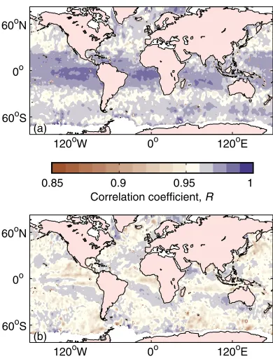
[85] The correlation coefficients ofW10andW37at each
grid point are shown in Figure 5 ; for W10 over 95% of
points have a correlation>0.95, while forW37this fraction
is 89%. The small number of cells below these thresholds is generally either close to land, or has a low count rate over the year. Correlation with wind speed is higher for W10, suggesting that more variability in W37can be
attrib-uted to factors other thanU10. Furthermore, becauseRis a
measure of the strength of a linear relationship, the correla-tions reported here may be biased low, more so in the case of W10 which has a more nonlinear dependence on wind
speed.
[86] The spatial structure of variations in correlation
coefficient differs between W10 and W37. Correlation
between U10 and W10 is highest in low-latitude regions.
Slightly lower values of R are found in the midlatitudes, where the variability in wind speed (and wavefield) is higher. Correlation is more variable forW37, with areas of
lower correlation found in both low average wind speed regions (equatorial Pacific) and regions where wind speed is on average much higher, but highly variable (Southern Ocean). We note that the spatial patterns in R are not explained by differences in theU10range which has
poten-tial to distort the statistic.
4.2. Dependence on Secondary Factors
[87] In the following analysis of the influence of
sec-ondary factors (Figures 6, 7, 9, and 10), the panels for normalized W10 and W37 have the same y scales for
easy comparison. We consider two main features in all the figures. One is the overall trend of normalized whitecap fraction W=W over the full range of possible values of each secondary factor and its deviation above and below unity. Another is the spread within a family of curves, color coded to show these deviations by wind speed bin.
0 5 10 15 20 25 30
10−3
10−2
10−1
100
101
U
10 (m s
−1
)
W
(%)
(a)
W
10
W
37
MM80 W(U
10)
Cal08 W(U
10)
GM11 W(U
10)
0 5 10 15 20 25
−3 −2 −1 0 1
Wsat
−
WCal08
(%)
(b)
10 GHz 37 GHz
0 5 10 15 20 25
−0.5 0 0.5 1 1.5 2
U
10 (m s
−1
) Wsat
−
WGM11
(%)
[image:12.610.142.470.75.319.2](c)
Figure 4. (a) Wind speed dependence of satellite-derivedW(W10andW37), twoW(U10)
parameteriza-tions from in situ data—that ofMonahan and O’Muircheartaigh [1980] (MM80) andCallaghan et al. [2008a] (Cal08)—and a W(U10) parameterization using satellite winds [Goddijn-Murphy et al., 2011]
(GM11). Error bars indicate the standard deviation. (b) The absolute difference betweenW10andW37and
4.2.1. Dependence of Whitecap Fraction on Wave Variables
[88] The variability of whitecap fraction as a function of
wave parameters is assessed by plottingW=W as a function ofHs,Tp, andMWS(Figure 6). It is evident that the influence of secondary factors onW10(Figures 6a, 6c, and 6e) is much
weaker than that onW37(Figures 6b, 6d, and 6f), in regards to
both the magnitude of the trends observed and the spread in these trends with wind speed. Additionally, secondary influen-ces are generally stronger with increasingU10.
[89] There is a small (6%), approximately linear,
increase in W10=W10 over the range of Hs (Figure 6a). W37=W37 increases much more withHs, particularly in the range 2 m<Hs<6 m (Figure 6b). In the range 3 m< Hs<5 m (depending on the wind speed), there is a leveling off, or even reduction in W37=W37 at low and moderate
wind speeds, while at the highest wind speeds, W37=W37
continues to increase, but at a much slower rate. The change in W37=W37 increases from 15% to 20% over the
range ofHswith increasing wind speed.
[90] As for Hs, the influence of Tp is small for W10
(Figure 6c) but larger forW37(Figure 6d). For normalized W10 there is little variation with Tp at low wind speeds, whereas at the highest wind speeds W10=W10 shows a
slight (5%) increase withTp. Likewise, deviations from the mean forW37=W37 over theTprange are much more pro-nounced for high wind speeds ; W37=W37 can increase by
as much as 20% as we move from a wave period of 5 s to 10 s. At lower wind speeds (U10<12 m s21), W37=W37
peaks at Tp511 s. For Tp513 s, changes to normalized Ware minimal.
[91] Mean wave slope combines information forHs and Tp, and so reflects joint changes in both variables. This variable serves as an indicator of the degree of wave development with MWS reducing as waves develop (MWS>0.03), reach wind-wave equilibrium (MWS
0.03), and finally become overdeveloped (MWS<0.03) [Bourassa et al., 2001]. Again, variations in normalized W10are small (Figure 6e). There is a clear peak in
normal-izedW37(Figure 6f) for a given wind speed, with the peak
values occurring in the range 0.025<MWS<0.035. At the lowest wind speeds, W37=W37 begins to rise again at
MWS>0.045. The peak in normalizedWat or close to the threshold marking wind-wave equilibrium indicates that sea states in equilibrium with the wind result in the largest values ofWat a given wind speed.
4.2.2. Degree of Wave Development
[92] The results in the previous section provide a coarse
assessment of changes toWdue to the wavefield, character-ized by three different variables. We examine the depend-ence ofWonHs,Tp, andMWSagain in Figure 7, but with further classification of the data as either wind sea (yellow/ red curves) or swell (blue curves). There are a small num-ber of cases where data cannot be classified as either swell or wind sea due to data being categorized as swell based on Hs and wind sea based on Tp, or vice versa. These cases (approximately 10%) are omitted from the analysis.
[93] The trends in normalized W10 due to change inHs are quite similar for wind sea and swell-dominated cases. For normalized W37 (panel b), there is some evidence to
suggest that the leveling off of normalized W with higher Hsis mostly confined to swell cases, whereas for wind sea conditions, normalizedWcontinues to increase although at a decreasing rate with increasingHs.
[94] Trends withTpare somewhat harder to evaluate due to the grouping of wind sea data at lowTp, and swell at high Tp. The influence ofTponW10at a given wind speed is
min-imal in swell conditions. A trend of increasingW10=W10is
seen for wind sea, whereas for swell there is little change. For W37, the largest deviations from the mean wind speed
behavior can be seen for wind seas at Tp<8 s, where seas are likely to be under-developed. Suppression of W37 is
strongest in this regime at the highest wind speeds; under these conditions, seas will be significantly under-developed.
[95] The results for MWS show that W10 is suppressed
slightly for wind sea and swell cases either side of MWS50.03, but with no clear separation between the behavior of the two cases. In conditions whereMWS>0.03, nearly allW estimates are classified as wind sea. Here nor-malizedW37increases withMWSat low winds, whereas at
higher wind speeds there is a strong decrease with increasing MWS. The latter results in a large suppression ofW37; in
such conditions, the magnitude of the wind in excess of equilibrium is at its largest [Bourassa et al., 2001]. We expect cases for which MWS<0.03 to correspond to well-developed seas; however,Westimates can still be classified as wind sea based on the classification usingHsandTp val-ues. In this MWSregime, there is a decrease in normalized W37with decreasingMWSfor both swell and wind sea cases,
although this decrease is more rapid in wind seas.
[96] We further assess the influence of the wavefield in
Figure 8 by classifying data as either swell, fully devel-oped, or wind seas, with wind seas further classified by
120oW 0o 120oE
60oS
0o
60oN
(a)
120oW 0o 120oE
60oS
0o
60oN
(b)
Correlation coefficient, R
[image:13.610.83.278.73.329.2]0.85 0.9 0.95 1
Figure 5. Global maps of cell-by-cell Pearson’s correla-tion coefficientRforU10and (a)W10, and (b)W37. Sources
forWandU10are listed in Table 1. Data comprise all
wave age (section 3.2.2). Using 1 m s21
bins to increase the number ofWestimates in individual bins, we calculate wind speed bin-averaged means,W, for each of the classes. The ratios W=Wfd are calculated for swell and three wave
age ranges of wind sea to quantify enhancement or suppres-sion ofW, at a given wind speed, due to under-developed (wind sea) or overdeveloped (swell) wave states. These are shown in Figure 8a forW10, and Figure 8b forW37.
[97] ForW10, deviations fromWfdin swell and wind seas
are almost negligible for 9 m s21
<U10<20 m s21. For
3 m s21<
U10<7 m s21, there is enhancement ofW10for
wind seas compared to fully developed sea states. However, this trend could be a result of the limitations of such a classi-fication for low wind speeds;Westimates forU10<7 m s21
are almost always classified as swell-dominated, with only 1–2% classified as fully developed. Therefore, calculation of Wfd at these wind speeds may suffer from poor statistics.
[98] ForW37(Figure 8b), deviations fromWfdare
gener-ally larger. Over much of the wind speed range, W is
enhanced in swell-dominated conditions, and suppressed in wind seas. Interestingly, for 7 m s21
<U10<13 m s21, the
largest suppression ofW37occurs in wind seas with highest
wave ages (25U31). At higher wind speeds (U10>14
m s21
),W37 is suppressed most in the youngest wind seas
(5U<20), withW 10% lower thanWfd.
4.2.3. Dependence on Other Environmental Factors
[99] The dependence ofWupon SST and the viscosity of
water are examined in Figure 9. The viscosity of water, although strongly related to SST, is a more fundamental quantity which takes into account the effect of salinity.
[100] The influence of SST onW10is very small, with a
slight reduction in W10=W10 at the highest values of SST
and for the highest wind speeds only (Figure 9a). Normal-ized W37 is near constant for SST < 20C, but drops off
rapidly for SST >20C (Figure 9b). Whitecap fraction is enhanced at a given wind speed by up to 12% at low tem-peratures. These deviations gradually decrease for SST
W
/
W
U
10 (m s
−1 )
4 6 8 10 12 14 16 18 20
0 0.01 0.02 0.03 0.04 0.05 0.06
0.85 0.9 0.95 1 1.05
MWS
(f)
0 0.01 0.02 0.03 0.04 0.05 0.06
0.85 0.9 0.95 1 1.05
MWS
(e)
5 10 15
0.75 0.8 0.85 0.9 0.95 1 1.05
T
p (s)
(d)
5 10 15
0.75 0.8 0.85 0.9 0.95 1 1.05
T
p (s)
(c)
0 2 4 6 8 10 12
0.8 0.85 0.9 0.95 1 1.05 1.1
Hs (m) (b)
0 2 4 6 8 10 12
0.8 0.85 0.9 0.95 1 1.05 1.1
[image:14.610.131.481.74.507.2]Hs (m) (a)
Figure 6. The dependence of (a, c, and e) W10=W10 and (b, d, and f)W37=W37 on (top) significant
ranging from 5 to 20C. Whitecap fraction is suppressed by
up to 25% for SST>20C.
[101] When plotted as a function of vw (Figure 9d), the effect on normalizedW37is as expected from the results for
SST. We stress the relatively small influence these factors have (no larger than 5%) on normalized W10 (Figure 9c).
There is however slightly more uniform behavior between the trends in normalized W10 andW37 at the higher wind
speeds (red), than that seen for SST.
[102] We explore the dependence ofWupon air
tempera-ture and the air-sea temperatempera-ture difference, DT, in Figure 10. The trends in bothW10andW37forTa(Figures 10a and 10b) are very similar to those found for SST ; this is most likely due to near surface air temperature coming into (near) equilibrium with SST over much of the ocean.
[103] The influence ofDTonWis less clear. The overall
influence on W10 (Figure 10c) is again less than 5% ; a
slight peak in normalizedW can be seen (at least for
mod-erate to high wind speeds) just below DT50, and a weak (5%) suppression for stronger unstable conditions. ForW37
(Figure 10d), at moderate and high wind speeds, normal-ized W decreases asDT goes from unstable toward stable conditions. At the lower wind speeds, W37=W37 shows
enhancement for strongly unstable conditions, then falls off quickly as we go from unstable to near neutral conditions, but then increases slightly when DT becomes positive. In the most stable of conditions, normalizedW37is suppressed
most at high wind speeds. The enhancement of normalized W37 is smaller in magnitude (5% at 14 m s21) than its
suppression (10% at 14 m s21
).
4.3. Relative Contribution of Forcing Factors
[104] The relative contribution of the different factors to
variability inWis evaluated using PCA. We plot, for both W10andW37, the variance explained by the first Principal
W/
W
U 10 (m s
−1 )
4 8 12 16 20
U 10 (m s
−1 )
4 8 12 16 20
0 0.01 0.02 0.03 0.04 0.05 0.06
0.8 0.85 0.9 0.95 1 1.05 1.1
MWS (f)
0 0.01 0.02 0.03 0.04 0.05 0.06
0.8 0.85 0.9 0.95 1 1.05 1.1
MWS (e)
5 10 15
0.75 0.8 0.85 0.9 0.95 1 1.05 1.1
T
p (s) (d)
5 10 15
0.75 0.8 0.85 0.9 0.95 1 1.05 1.1
T
p (s) (c)
0 2 4 6 8 10 12
0.8 0.85 0.9 0.95 1 1.05 1.1
H
s (m) (b)
0 2 4 6 8 10 12
0.8 0.85 0.9 0.95 1 1.05 1.1
H
s (m) (a)
[image:15.610.131.482.74.505.2]wind sea swell−dominated
Component (PC1) for wave and wind-wave variables (Fig-ure 11a), and other environmental factors (Fig(Fig-ure 11b). We consider all variables, including those which have an explicit dependence on wind speed—such as the two Reyn-olds numbers. The variables are ordered by the percent var-iance explained by PC1.
[105] The highest ranking variable is wind speed for both
W10 and W37. Two of the wind-wave variables (the
breaking-wave and roughness Reynolds numbers) perform almost as well, with significantly higher scores than the other wind-wave variables considered. The next best per-forming wave variable isHs, followed byU, andMWS.Tp accounts for only 50% of the variance of both W10 and W37.
[106] Ta, SST, andvwall describe roughly the same per-cent variance. Notably, these three variables also show the biggest difference in variance explained by PC1 between W10 and W37, accounting for 4% more variance in W37
than inW10. This supports the findings in section 4.2.3 that
SST (or viscosity of water) has a more pronounced impact onW37than onW10. Note that this difference is not as large
as one might expect because here we consider estimates covering almost the whole globe, whereas larger changes to W resulting from SST changes are probably confined to very warm waters (equatorial regions). In the case of the breaking wave Reynolds number and the roughness Reyn-olds number, variance explained by PC1 forW37is slightly
lower than that for W10. Because both Reynolds numbers
combine information on the wind field and wavefield, they may be better predictors of the variability of active foam 0.85
0.9 0.95 1 1.05 1.1 1.15
(a) W
10
0 5 10 15 20
0.85 0.9 0.95 1 1.05 1.1 1.15
U
10 (m s
−1)
W
/
W
fd
(b) W
37
wind sea (5 ≤Φ < 20)
wind sea (20 ≤Φ < 25)
wind sea (25 ≤Φ≤ 31)
[image:16.610.85.273.73.363.2]swell
Figure 8. Ratio of wind speed averaged (a)W10 and (b) W37toWfd for swell and wind sea cases, with wind sea
fur-ther classified by wave age.
W/
W
U
10 (m s
−1)
4 6 8 10 12 14 16 18 20
0.8 1 1.2 1.4 1.6 1.8
x 10−6
0.75 0.8 0.85 0.9 0.95 1 1.05 1.1
ν w (m
2/s) (d)
0.8 1 1.2 1.4 1.6 1.8
x 10−6
0.75 0.8 0.85 0.9 0.95 1 1.05 1.1
ν w (m
2/s) (c)
0 5 10 15 20 25 30
0.75 0.8 0.85 0.9 0.95 1 1.05 1.1
SST (oC)
(b)
0 5 10 15 20 25 30
0.75 0.8 0.85 0.9 0.95 1 1.05 1.1
SST (oC)
(a)
Figure 9. The dependence of (a and c)W10=W10and (b and d)W37=W37 on (top) SST, and (bottom)
[image:16.610.133.480.415.726.2]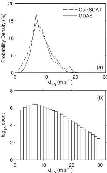

![Figure 4.(a) Wind speed dependence of satellite-derived[2008a] (Cal08)—and ations from in situ data—that of(GM11)](https://thumb-us.123doks.com/thumbv2/123dok_us/7984224.203461/12.610.142.470.75.319/figure-wind-speed-dependence-satellite-derived-cal-ations.webp)