This is a repository copy of
Low-cost wind resource assessment for small-scale turbine
installations using site pre-screening and short-term wind measurements
.
White Rose Research Online URL for this paper:
http://eprints.whiterose.ac.uk/81528/
Version: Accepted Version
Article:
Weekes, SM and Tomlin, AS (2014) Low-cost wind resource assessment for small-scale
turbine installations using site pre-screening and short-term wind measurements. IET
Renewable Power Generation, 8 (4). 349 - 358. ISSN 1752-1416
https://doi.org/10.1049/iet-rpg.2013.0152
eprints@whiterose.ac.uk https://eprints.whiterose.ac.uk/ Reuse
Unless indicated otherwise, fulltext items are protected by copyright with all rights reserved. The copyright exception in section 29 of the Copyright, Designs and Patents Act 1988 allows the making of a single copy solely for the purpose of non-commercial research or private study within the limits of fair dealing. The publisher or other rights-holder may allow further reproduction and re-use of this version - refer to the White Rose Research Online record for this item. Where records identify the publisher as the copyright holder, users can verify any specific terms of use on the publisher’s website.
Takedown
If you consider content in White Rose Research Online to be in breach of UK law, please notify us by
1
Low-Cost Wind Resource Assessment for Small-Scale Turbine
Installations Using Site Pre-Screening and Short-Term Wind
Measurements
S. M. Weekes* and A. S. Tomlin
Doctoral Training Centre in Low Carbon Technologies, Energy Research Institute, School of
Process, Environmental and Materials Engineering, University of Leeds, Leeds, LS2 9JT, UK
*E-mail: S.M.Weekes08@leeds.ac.uk
A two-stage approach to low-cost wind resource assessment for small-scale wind installations
has been investigated in terms of its ability to screen for non-viable sites and to provide
accurate wind power predictions at promising locations. The approach was implemented as a
case study at ten UK locations where domestic-scale turbines were previously installed. In stage
one, sites were pre-screened using a boundary layer scaling model to predict the mean wind
power density, including estimated uncertainties, and these predictions were compared to a
minimum viability criterion. Using this procedure, five of the seven non-viable sites were
correctly identified without direct onsite wind measurements and none of the viable sites were
excluded. In stage two, more detailed analysis was carried out using three months onsite wind
measurements combined with measure-correlate-predict (MCP) approaches. Using this
process, the remaining two non-viable sites were identified and the available wind power density
at the three viable sites was accurately predicted. The effect of seasonal variability on the MCP
predicted wind resource was considered and the implications for financial projections were
highlighted. The study provides a framework for low-cost wind resource assessment in cases
2
1 Introduction
Small-scale wind energy is a renewable energy technology with exciting prospects as we move
towards a low carbon energy future. In order to achieve widespread deployment however, it is
vital to develop tools capable of predicting the wind resource quickly, cheaply and accurately [1].
These tools will ensure that turbines are installed in locations which maximize the financial and
environmental benefit and will allow customers to choose between competing low carbon
technologies with confidence.
The need for suitable wind resource assessment tools has been highlighted by several studies.
In 2008, Encraft along with a number of partners carried out a UK study of 26 building mounted
small wind turbines, known as the Warwick Wind Trials [2], to investigate turbine performance in
a variety of locations. The study highlighted the challenge of accurately predicting the potential
wind resource using simple methods such as the NOABL (numerical objective analysis of
boundary layer) [3] wind speed database. Among the study’s conclusions were that more work
was needed in creating robust methods for predicting mean wind speeds and wind speed
distributions, particularly in urban areas [2]. Following the Warwick Wind Trials, in 2009 the
Energy Saving Trust (EST, a UK foundation working in partnership with government and
business) [4], completed a larger field trial of domestic-scale wind turbines. The field trial
monitored the performance of 57 small-scale (0.4 – 6 kW) pole and building mounted wind
turbines in a variety of locations throughout the UK over a one year period with the aim of
assessing turbine performance at a variety of sites. While the results showed a promising
potential for small turbines installed at appropriate locations, a large number of the monitored
sites revealed wind speeds and turbine performance that were significantly lower than expected
[5, 6].
In the large-scale wind industry, wind resource assessment is well established and typically
3
data are used to make reliable predictions of the long-term wind energy resource as required by
financial investors. In the small-scale wind industry these timescales are often impractical and
the impact of such a measurement campaign on the total investment cost may be prohibitively
high. In the absence of long-term onsite measurements, indirect methods must be used.
Indirect approaches may be broadly divided into modelling or data-led techniques. Simple
modelling techniques, such as boundary layer scaling models, can be particularly efficient since
after development and validation, onsite wind speed measurements are generally not required
in order to make predictions. However, since uncertainties exist at each stage of the modelling
process [8], the final predictions may not reach the accuracy required by investors [9]. In
contrast, data-led techniques which involve direct wind speed measurements at the site of
interest may result in more accurate resource predictions but they are more costly and time
consuming to implement. One way of leveraging the advantages of both of these approaches is
through the deployment of simple modelling techniques to screen sites for suitability followed by
more detailed assessment of promising locations using short-term onsite wind speed
measurements.
To investigate the feasibility of such an approach we have performed a case study of a subset
of the installations involved in the EST field trial. Since each of these sites represents a location
that was deemed suitable for the installation of a small-scale wind turbine, they provide an ideal
opportunity to investigate the implementation of wind resource assessment tools in realistic
scenarios. The case study is focused exclusively on assessing the wind resource at each site,
as measured by onsite anemometry, and investigating the degree to which this may be
predicted using a combined modelling and data-led approach.
The work addresses the following issues: (I) Investigation of the appropriateness of a boundary
4
identifying locations worthy of further investigation. Specifically, we address the question as to
whether, given the inherent uncertainties of such approaches, they can be of sufficient accuracy
to screen sites based on a viability criterion. (II) Quantification of the propagated errors in the
predicted wind resource arising from uncertainties in the model input parameters and
identification of the relative importance of these uncertainties using a global sensitivity analysis.
(III) Estimation of the added value, in terms of the accuracy of the predicted wind resource, of
implementing a very short-term onsite measurement campaign at promising sites to supplement
the modelling approach.
2 Methodology
The two-stage approach to wind resource assessment proposed in this study, following the
recommendations from previous work [9, 10], can be summarised as follows:
(I) Site pre-screening: a boundary layer scaling model is applied at a potential wind
turbine site to predict the mean wind speed at the proposed hub height of the turbine.
The wind speed is used to derive a predicted mean wind power density and an
associated uncertainty and this is compared against a predefined minimum viable
value. If the predicted value is below this minimum, the site is deemed non-viable
and excluded from further analysis.
(II) Detailed analysis: For sites passing the pre-screening stage, short-term (3 months)
onsite measurements are used along with MCP analysis to make a more precise
prediction of the available wind resource and to identify any remaining non-viable
sites. In practice, short-term onsite measurements may be obtained using a mobile
meteorological mast or portable LiDAR (light detection and ranging) equipment
5
Using this approach, the additional time and investment required for onsite measurements are
not wasted on sites which are clearly non-viable and are instead concentrated on sites that have
already been identified as having a good potential. The success of this approach is investigated
by comparing predictions made at stages I and II with onsite wind data obtained over a 12
month period at the selected UK sites.
The following sections outline each stage of the process in more detail. Firstly, the
meteorological measurements and the geographical locations of the sites are described. Next,
details are given of the boundary layer scaling model and MCP approaches used to make wind
resource predictions, including specific factors related to short onsite measurement periods.
Finally, a viability criterion for use in the site pre-screening stage is developed.
2.1 Meteorological measurements
This study utilises wind data collected during the EST field trial of domestic-scale wind turbines
mentioned previously. For the duration of the field trial, five minute averages of wind speed
(resolution 1 ms-1) and wind direction (resolution 1 ) were collected at each turbine location
using ultrasonic anemometers located at a height close to that of the turbine hub [5]. Following
the completion of the field trial, these data were transferred to the UK trade body RenewableUK
for the purpose of further dissemination to the research community. Data for the current study
were obtained directly from this source.
In order to fully investigate the wind resource assessment approaches, ideally wind data
covering a number of years are used to account for both seasonal and inter-annual variations.
However, given the relative infancy of the small-scale wind industry, long-term wind data from
small turbine installations are not widely available. In the absence of long-term wind data,
measurements covering a full year with a relatively strict data coverage criterion are desirable.
6
period was used in order to properly account for seasonal variability. Of the 57 fully monitored
sites in the field trial, only 10 sites (referred to here as target sites) were found to achieve this
criterion. While this represents a relatively small sample, the 10 sites were located in a range of
terrains (urban, sub-urban, rural and coastal) and at a variety of heights above ground level
(5-12 m). Hence they are a useful starting point in investigating general trends associated with the
application of resource assessment tools to real-world, small-scale wind turbine sites.
To implement the MCP approaches, concurrent measurements from nearby reference sites are
required. Reference sites were selected from the UK Meteorological Office (Met Office)
anemometer network [12] on the basis of their proximity to the target sites and the openness of
the terrain, as judged by satellite images. In cases of pairings with coastal target sites,
preference was given to coastal reference sites. The Met Office reference site data used in this
work consisted of hourly averages of wind speed (resolution 1 knot = 0.51 ms-1) and direction
(resolution 10 ) recorded at a height of 10 m above ground level and averaged over a complete
hour. Due to the different averaging periods for the Met Office reference and EST target sites,
the EST observations were processed to obtain hourly averages of wind speed and direction.
These data were time-aligned with the hourly Met Office observations resulting in concurrent
data sets for each reference and target site pair, covering the period April 2008 – March 2009.
The geographical locations of the target and reference sites are shown in Figure 1 and further
7
[image:8.612.73.329.70.449.2]Figure 1: Approximate geographical locations of meteorological monitoring sites. Circles represent target sites (T) and stars represent reference sites (Rf).
Table 1: Summary of meteorological monitoring sites. is the observed mean wind speed as obtained from onsite wind speed measurements over a 12 month period, is the target site anemometer height above ground level and is the separation between the target and reference sites.
© Crown copyright/database right 2011. An Ordnance Survey/EDINA supplied service.
Rf4 T4
T1
T7
T2
T8 T9
T3 T5
T6 T10
Rf1
Rf6
Rf2
Rf7
Rf3
Rf5 Rf8
Target sites Reference sites
Site Terrain obs(ms-1) h(m) Site Terrain d(km)
T1 Coastal 1.8 7.7 Rf1 Coastal 43
T2 Rural 4.9 8.0 Rf2 Rural 36
T3 Rural 2.4 9.8 Rf3 Semi-rural 15
T4 Coastal 3.6 5.0 Rf4 Coastal 8
T5 Sub-urban 2.2 11.3 Rf4 Coastal 20
T6 Urban 2.5 9.0 Rf5 Semi-rural 31
T7 Coastal 3.0 7.7 Rf6 Coastal 3
T8 Rural 4.3 7.0 Rf7 Rural 72
T9 Rural 4.6 7.0 Rf7 Rural 59
8
2.2 Boundary layer scaling model
The modelling approach used in this work is based on a semi-empirical (SE) model first
developed by the UK Met Office, which uses the principles of boundary layer meteorology to
predict the spatially averaged mean wind speed without the need for direct meteorological
measurements [8]. The model is also conceptually similar to that applied by Heath et al. [13] to
investigate the potential energy output from a hypothetical micro-wind turbine installation in
London. While the study by Heath et al. also investigated the detailed effects of building scale
wind flows in urban areas using computational fluid dynamics, the SE methodology considers
only the spatially averaged flow and is applicable to a variety of terrain types. The SE model
was previously the subject of a detailed study [9] that evaluated its real-world performance and
suggested modifications to improve the accuracy of its predictions. In this work, we have
implemented the model along with the modifications recommended in reference [9]. Since a
detailed description of the model is available elsewhere [8, 9], here we present only a summary
of the pertinent steps.
For wind flows close to the Earth’s surface, under neutral stability conditions and in the constant
stress layer of flow, the vertical profile of the horizontal mean wind speed can be described by
[14]:
Equation 1
where is the spatially averaged mean wind speed at height , is the friction velocity with
units [ms-1], = 0.4 is the Von Karman constant and and are the displacement height and
9
Note that given the wind speed at some reference height, Equation 1 can be applied to calculate
the wind speed at some new height without explicit knowledge of , providing the remaining
parameters are known. The variables and , collectively called the aerodynamic parameters,
are of particular interest since they describe the characteristics of the surface roughness. The
displacement height, in effect, shifts the origin of the vertical z-axis to a height in order to
account for the blocking effect of local obstacles, while the roughness length serves as a
parameterization of the drag force exerted by the roughness elements. These parameters are
non-trivial to estimate, particularly in complex environments [15, 16].
In the current methodology, we require both regional estimates (over several kilometres) and
local estimates (over several hundred metres) of the aerodynamic parameters. Regional
estimates are obtained using the blending method of Mason [17] where spatially averaged
values for and are derived from the fractionally weighted land cover at the location of
interest [9]. As an extension of the Met Office approach, we increase the size of the regional
area from a 1 km x 1 km to a 4 km x 4 km grid square centred on the site of interest in order to
account more fully for contributions to the regional surface roughness. In addition, directionally
dependent surface roughness is incorporated through division of the grid square into a further
four subsectors. The subsectors are then used to estimate the roughness of the upwind fetch
within a 90 degree angular sector. This approach has been shown to be of particular
importance in cases where there are sudden changes in roughness such as at coastal sites [9].
The starting point for estimates of the local aerodynamic parameters is a visual assessment of
the local (~250 m x 250 m) site character using satellite images. In line with the Met Office
approach [8], the site is classified according to one of seven categories (high height and density
residential, low height and density residential, open country etc.) and appropriate estimates of
10
the aerodynamic parameters, as well as the wide range of possible site characteristics, these
estimates have a high degree of uncertainty [8, 15].
Using the principles outlined above, a methodology can be developed to predict the spatially
averaged, hub-height wind speed at a specific site given a reference wind speed at a known
height. The approach may be summarized as follows [9]:
(I) For a specific UK location defined on a grid of 1 km2, a reference mean wind speed at 10 m
above open, level ground, is obtained from the Met Office National Climate Information Centre
(NCIC) database [18]. Since the NCIC wind speeds are based on a 30 year average over the
period 1971 – 2000, and the EST observations used for validation of the method are based on a
single year of wind data, a correction factor was applied to account for inter-annual variability.
Three of the reference sites used in this study (Rf1, Rf4 and Rf8) had suitably long-term data
records and these were used to compare the mean wind speeds for the periods 1971 – 2000
and April 2008 – March 2009. Based on this comparison, the NCIC wind speeds were multiplied
by a correction factor of 0.97 in order to reflect the lower wind speed observations during the
EST observation period. A similar approach was used by Sissons et al. to correct the EST
observations relative to a 10 year mean [6].
(II) The reference wind speed is then scaled up to a height of 200 m, where the flow is
considered independent of the local and regional roughness. This is achieved using Equation 1
along with the aerodynamic parameters = 0.14 m and = 0, representative of open country.
Note that while a smaller roughness length (~0.03 m) would be expected for short-grass,
extended regions of short grass without interruption from hedges and bushes are relatively
unlikely in UK rural areas [8]. Hence, in practice, = 0.14 m is considered more representative
11
(III) The wind speed is then scaled down to an intermediate height known as the blending height
(the height at which the flow is ‘horizontally homogenous and in equilibrium with the local
surface’ [17]), again using Equation 1. Here, aerodynamic parameters representative of the
regional area are applied. The blending height is taken to be the larger of 10 m or two times the
maximum canopy height of any land use within the regional grid square. This is in accordance
with previous studies [8, 9] and is based on the assumption of a blending height of 2-5 times the
height of the roughness elements [19]. Note that strictly this height will also be a function of the
distance from the roughness change, although this may be impractical to implement in a simple
automated approach designed to be applied to multiple sites.
(IV) Equation 1 is then applied a final time to scale the mean wind speed down to the turbine
hub-height using aerodynamic parameters representative of the local area. A Weibull wind
speed distribution [20] is used along with the predicted mean wind speed to enable the wind
power density to be estimated.
It is important to note that the above methodology is formulated to predict only the spatially
averaged mean wind speed and associated wind power. While for well exposed locations this is
likely to be a reasonable approximation, for turbines mounted close to buildings or other
obstructions, there can be significant local deviations from this spatial average [13, 21]. These
deviations will depend on factors such as the geometry of the obstructions, the position of the
turbine within a building array and the prevailing wind direction. Such factors must be assessed
using suitable correction factors or detailed flow modelling [13], both of which are likely to be
highly site specific. These corrections are beyond the scope of the boundary layer scaling model
presented here which is designed to be implemented using simple parameterisations of the
regional and local surface characteristics. However, it has previously been demonstrated [21]
12
speed can be considered as a good approximation of the lower bound to the wind speed
experienced at the proposed turbine location.
2.3 Quantifying prediction uncertainty
As with any modelling approach, the final mean wind speed and wind power density predictions
are subject to uncertainties. These arise firstly from assumptions and simplifications inherent in
the model itself and secondly from uncertainties in the model input parameters. In the following
discussion we are concerned with the uncertainties arising from the latter. At each stage of the
model implementation, appropriate input parameters must be chosen. These include the input
reference wind speed, the regional and local aerodynamic parameters, the blending height and
the Weibull shape factor required to construct a distribution of wind speeds. Uncertainties in the
values of these parameters combine to produce uncertainties in the final model predictions.
Since accurately estimating the regional and local aerodynamic parameters is known to be
particularly challenging, these are considered as the dominant error source in the mean wind
speed prediction. These errors combine with the uncertainty in the Weibull shape factor to
produce errors in the final wind power prediction.
To quantify the effect of these uncertainties, a quasi-random sampling approach, implemented
in the MATLAB programming environment, was applied to each individual site prediction using a
Sobol sequence [22]. A Sobol sequence is a low discrepancy numerical sequence that allows a
multi-dimensional parameter space to be filled efficiently with minimal gaps. Given a model
output based on a number of input parameters, sampling using a Sobol sequence allows an
efficient estimation of the overall output uncertainty related to various combinations of input
parameters. For the mean wind speed prediction, a five dimensional Sobol sequence of length
1024 was used to sample a range of values for the four aerodynamic parameters of regional
and local and as well as the blending height. An approximate uncertainty in the default
13
recommended in a comprehensive study by Grimmond and Oke [15]. A range of +/- 35% was
also used for the blending height since it was found that larger ranges resulted in parameter
combinations within the Sobol sequence that were not physically viable. For the mean wind
power density prediction, a six dimensional Sobol sequence of length 1024 was used, with the
Weibull shape factor as the sixth sampling parameter. Weibull shape factors in the range =
1.5 - 2.3 were employed based on the results of a previous study that obtained Weibull shape
factors from 38 UK sites [9]. Using such a sampling approach gives distributions of wind speed
and power density predictions which reflect the propagation of uncertainties within the input
parameters to the outputs. Presented here are the mean predictions of wind speed and power
density from these distributions with uncertainties represented by plus or minus twice the
standard deviation (+/- 2 ) across the 1024 samples.
In addition to estimating the overall prediction uncertainty using a sampling approach, it is also
informative to understand the relative contributions to this uncertainty from each of the six input
parameters. Ultimately, such information could be used to improve the model by obtaining better
estimates of the most significant parameters. To investigate these contributions, a global
sensitivity analysis was conducted using the GUI-HDMR (graphical user interface – high
dimensional model representation) software tool in MATLAB, which has successfully been
applied in a number of environmental modelling contexts [23]. Given a quasi-random sample
across specified input parameters, (in the present case these are obtained from a
six-dimensional Sobol sequence as described above), and the corresponding model output
(predicted wind power density) the GUI-HDMR applies a variance-based sensitivity analysis to
estimate the relative importance of each of the input parameters. The output sensitivity to each
parameter is quantified by means of first-order , and second-order , sensitivity indices. The
first-order indices represent the fractional contribution of the parameter to the output
14
pairs of input parameters. The sum across all indices should be 1. In the current study, first- and
second-order indices were calculated for each of the ten test sites. Second-order effects were
however found to be small and hence are not considered in the following discussion. A detailed
description of the GUI-HDMR is available in reference [23].
2.4 Measure-correlate-predict approaches
The measure-correlate-predict (MCP) technique is a data-led method which increases the value
of short-term wind measurements recorded at a potential wind energy site by correlating these
with concurrent data recorded at a nearby reference site. In this work, the short-term concurrent
wind measurements at the target and reference sites are referred to as the training data. The
correlation obtained from the training data is applied to long-term historical data records from
the reference site to construct a long-term time series of predicted wind speeds at the target
site. The long-term predicted time series can then be used to extract statistical descriptors of the
wind resource including the mean wind speed and average wind power density. Since long-term
wind speed records are routinely held by airports and national weather forecasters, this
technique provides a means of reducing the onsite measurement time required at the target
site.
MCP is already utilized in the large-scale wind industry where the relationship between the
reference and target sites is typically estimated from a measurement period covering a year or
more [24]. However, recent studies [10, 11] applying the MCP approach to measurement
periods of much less than one year have shown promising results providing appropriate
precautions are taken relating to seasonal variability and data coverage. Based on these
observations, we have applied the MCP techniques of variance ratio regression (VR) and linear
regression (LR) to achieve a more detailed investigation of the available wind power at each
site. Full details of the MCP approaches can be found in reference [10], hence only a brief
15
2.4.1 Linear regression
A linear correlation between concurrent wind speed observations at the reference and target
sites, and , can be described by the linear equation [25]:
Equation 2
where and represent the regression coefficients obtained by minimising the sum of squares
of the residuals and is an error term which represents the residual scatter about the mean
prediction. Given a linear regression on the observed data, a predicted target site wind speed
, can be obtained using the extracted regression parameters and the concurrent reference
site wind speed . To account for the residual scatter about , which is important in
accurately predicting the mean wind power density [10], the residual scatter term , is modelled
using a zero-mean Gaussian distribution of the form:
Equation 3
Here represents the sample standard deviation of the residuals as estimated from the
training data using the expression [26]:
Equation 4
16
A representation of the residual scatter is reconstructed by adding random draws from the
Gaussian distribution described by Equation 3 to the individual mean predictions at the
target site.
2.4.2 Variance ratio method
In the case of simple LR where the error term is not included, it is known that the variance of
the predicted wind speeds about the mean is not properly accounted for. In response to this,
Rogers et al. [27] proposed a variation of simple LR. In this approach, the predicted target site
wind speeds are linearly related to the observed reference site wind speeds by the expression:
Equation 5
where and are the sample standard deviation about the mean and at the
target and reference sites respectively, as estimated from the training period. Since the ratio
represent the gradient of the linear regression in Equation 5, this approach is referred
to as the variance ratio (VR) method [27].
To account for variations in the upwind surface roughness, and in line with previous approaches
[10, 27], the LR and VR approaches were applied sector-wise to data which had been binned
into 30 degree angular sectors according to the reference site wind angle. This results in 12
separate regression equations for each reference/target site pair. For sectors that have
recorded less than 20 data entries during the training period, a global fit was applied to all
17
2.4.3 Application of MCP approaches to data of limited length
In order to rigorously test the success of new MCP approaches, non-overlapping periods should
be used for training the algorithms and testing their performance. This implies the use of wind
data covering multiple years. However, the aim of the current case study is not to test new MCP
approaches but rather to establish to what degree the specific 12 month wind resource,
covering the period April 2008 – March 2009, may have been predicted if the measurement
period was restricted to just three months. While this negates the need for wind data covering
multiple years, the fact that the wind data used in this study cover a single year leads to two
specific challenges related to seasonal variability which must addressed. Firstly, seasonally
varying synoptic weather patterns are likely to affect the regression parameters extracted during
the 3 month training period and secondly, since the total data period covers just 12 months, the
use of non-overlapping training and testing periods will result in seasonal bias.
To account for these issues the following approach was used: (I) regression parameters were
estimated using a full 3 month training period, (II) based on the extracted parameters, the MCP
approaches were implemented to predict a time-series of wind speeds for the remaining 9
months of the year, (III) an annual wind resource prediction was made by combining the 9
months of predicted wind speeds with the 3 months of measurements during the training period.
These steps represent a single prediction of the annual wind resource based on just 3 months
measurements. To account for seasonal variability, the training period was next shifted by one
month and the above steps were repeated to obtain a second prediction of the annual wind
resource. This process was repeated for all months of the year in order to include training
periods covering all combinations of seasons. This process results in 12 separate predicted
wind speed time series for the period April 2008 – March 2009. This approach replicates the
range of possible predictions that may be obtained using any arbitrary 3 month training period to
18
2.5 A viability criterion
In this work, the modelling (SE) and data-led (LR and VR) approaches to wind resource
assessment were applied in a two-stage process involving site pre-screening followed by more
detailed wind power predictions. The pre-screening stage involved the application of only the SE
model in order to test sites against some criterion of viability. Sites passing the criterion were
judged to be worthy of more detailed investigation using onsite measurements and the MCP
approaches.
Defining a viability criterion is non-trivial since one may consider environmental viability (the
ability of a turbine to produce sufficient energy to repay its embedded carbon) and financial
viability, (the ability of a turbine to produce sufficient energy to repay the financial investment).
These will vary greatly depending on the materials and costs of specific turbines as well as the
availability and level of government sponsored financial incentives. In the context of small-scale
wind turbine installations, recent studies concerned with assessing city-wide wind energy
potential [28, 29] have used a mean wind speed viability criterion of 4-5 ms-1, these values are
also in line with industry advice offered by the UK trade body RenewableUK [30].
While a minimum mean wind speed is a useful starting point, the available wind power will
depend both on the mean wind speed and the distribution of wind speeds at the proposed site.
Hence, it is useful to express this criterion in terms of a minimum wind power density. Assuming
a Weibull distribution of wind speeds, the mean Betz power density in the wind , can be
expressed as [31]:
19
where the factor 16/27 represents the Betz limit, = 1.225 kgm-3 is the air density, is the
gamma function, is the Weibull shape factor and represents the mean of the cubed wind
speeds, (as opposed to the cube of the mean wind speed, ).
Using a minimum mean wind speed of 4 ms-1 and a Weibull shape factor = 1.9, as
representative of UK sites [9], this equates to a viability criterion of ≥ 47 Wm-2. An intuitive
feel for this number can be gained through some simple calculations. Assuming 50% of the
available Betz power can be converted to electrical power [4], (this is a broad approximation
since efficiency will vary with wind speed and turbine design), for a small-scale turbine with a
blade diameter of 2 m, this equates to an average power production of 74 W and an annual
energy production of 647 kWh. For a larger turbine with a blade diameter of 6 m, this equates to
an average power production of 664 W and an annual energy production of 5821 kWh. Note
that efficiencies may be reduced for building mounted turbines in urban areas due to turbulent
wind flows. In the following analysis, the minimum power density criterion of ≥ 47 Wm-2 is
applied to screen for viable sites. Locations predicted to have a power density below this value
are deemed non-viable and are excluded at the site pre-screening stage.
3 Results and Discussion
The first stage in assessing the wind resource is to obtain a prediction of the mean wind speed.
Figure 2 shows the predicted and observed mean wind speeds at the ten target sites over the
full 12 month period using the SE model as well as the MCP approaches of LR and VR. As a
benchmark, wind speeds from the NCIC database, used as input for the SE model, have also
been included. Since the NCIC wind speeds represent expected values over open terrain, these
have been scaled to the anemometer height using Equation 1 with no correction for the local
site characteristics (i.e. using aerodynamic parameters representative of open country = 0.14
20
predicted wind speed ranges rather than point values, representing the variable predictions
obtained using training data from different seasons. The MCP predictions cover a range of +/-
0.1 to 0.6 ms-1 across the different seasons using LR and this range tends to be centred close to
the observed values. The SE predictions exhibit significantly more scatter with regular over or
under predictions and an estimated uncertainty of +/- 0.3 to 0.7 ms-1 reflecting the uncertainty in
the input aerodynamic parameters. Despite these uncertainties, SE offers a notable
improvement over the uncorrected NCIC wind speeds, thus highlighting the value of the model.
Note that in the case of the SE predictions, not all the error bars cross the observed values,
(represented by the dotted line) indicating that some modelling uncertainties are unaccounted
for. This is not surprising since the process detailed in Section 2.3 only accounts for
uncertainties in the model input parameters and does not consider the specific model
assumptions or the fact that the mean wind speed predictions are a spatial average. The
unaccounted for errors are particularly noticeable for sites with a low observed mean wind
speed, indicating that local obstructions to the wind flow may be causing local sheltering of
these sites.
1 2 3 4 5 6 7
1 2 3 4 5 6 7
p
red
(m
s
-1)
obs(ms-1)
21
Figure 2: Predicted ( ) verses observed ( ) mean wind speeds at ten target sites using the SE
model (circles) and the MCP approaches of LR and VR (solid bars). The NCIC wind speeds scaled to anemometer height (filled circles) are also shown. The error bars attached to the SE predictions represent an uncertainty of +/- 2 . The MCP predictions are represented by solid bars indicating the range of predictions obtained for training data collected during different seasons. The dotted line represents a one-to-one relationship.
3.1 Site pre-screening
In order to apply the site pre-screening procedure, an estimate of the mean wind power density
, must be made for each target site. Figure 3 shows the observed and predicted values of
for each site based on the SE mean wind speed predictions. The mean and uncertainty ranges
for the predicted are obtained using Equation 6 along with the sampling process outlined in
Section 2.3 to account for uncertainties in the input parameters. On average, the calculated
uncertainty in is around +/- 50% with higher values observed at complex urban sites and
lower values observed at open rural sites. As with the mean wind speed predictions, the
estimated uncertainties in do not cross the observed values in some cases indicating
additional errors that are not accounted for in the sampling process. In particular, there appears
to be a net positive bias in the predicted mean wind speed and wind power density for the sites
considered in this study. Despite this however, the predictions and their associated uncertainties
22
Figure 3: Observed and predicted mean wind power density , for ten target sites obtained using an SE model. The circles represent the mean prediction and the error bars show an uncertainty of +/- 2 . The dotted horizontal line represents the viability criterion of ≥ 47 Wm-2.
To implement the site pre-screening process we wish to identify sites which are likely to be
unsuitable as judged by the viability criterion of ≥ 47 Wm-2. To reduce the likelihood of
mistakenly excluding viable sites, only sites where even the most optimistic wind power
prediction is below the viability criterion should be excluded. Taking this approach, all sites
where the predicted plus the associated uncertainty (top of each error bar) is below the
viability criterion should be deemed unsuitable.
Figure 3 shows that based on this methodology, five of the ten sites (T1, T3, T4, T5 and T6)
would be deemed non-viable and excluded from further investigation. Figure 3 also shows that
based on the onsite wind speed observations, these exclusions would be correct since none of
these sites reach the minimum power density criterion. Given that turbines were installed at all
ten sites, this result shows that even a site pre-screening process involving no onsite
measurements would have been very valuable in identifying these sites at an early stage and
avoiding further investments.
0 20 40 60 80 100 120 140 160
T1 T2 T3 T4 T5 T6 T7 T8 T9 T10
p
d(w
m
-2)
23
Of the five sites that passed the viability criterion, onsite observations show that three (T2, T8
and T9) exhibited a ≥ 47 Wm-2 while the remaining two fell well below this level. Hence, for
the sites considered in this study, the pre-screening approach has successfully predicted five
out of the seven non-viable sites without excluding any of the three viable sites. Based on a less
conservative approach, namely the mean wind power prediction, all seven non-viable sites
would have been correctly excluded, although two of these (T7 and T10) only marginally so. It is
clear from Figure 3 that there are significant errors and uncertainties in the predicted using
the SE approach, indicating that it would be unwise to make financial projections based on
these values. However, when used as a site pre-screening tool, the accuracy requirements are
less strict requiring only that the general trends be predicted.
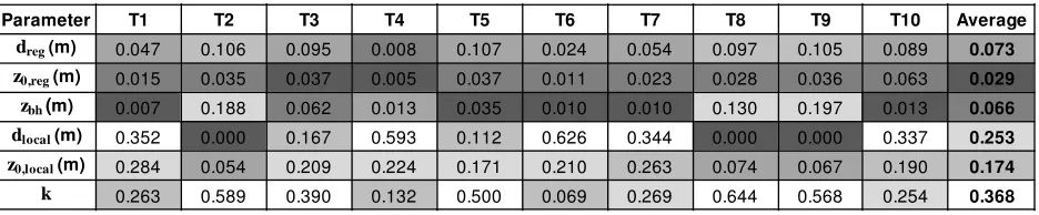
[image:24.612.75.543.447.544.2]3.2 Global sensitivity analysis
Table 2 shows the first-order sensitivity indices calculated using GUI-HDMR, for each of the six
model input parameters at each site with respect to the output prediction . Parameters with
larger index values (lighter shading) indicate that the output is more sensitive to that parameter.
Table 2: First-order sensitivity indices for the six SE model input parameters of regional displacement
height and roughness length ( , ), blending height ( ), local displacement height and roughness length ( , ) as well as Weibull shape factor at each target site. Indices are calculated with respect to the output of predicted wind power density ( ). Shading indicates the relative contribution of each parameter to the uncertainty, from smallest (dark) to largest (light).
On average, the single parameter with the highest sensitivity index is the Weibull shape factor
. However, the combined contribution of the remaining five parameters related to the mean
wind speed prediction is proportionally larger, highlighting the importance of these parameters.
Parameter T1 T2 T3 T4 T5 T6 T7 T8 T9 T10 Average
dreg (m) 0.047 0.106 0.095 0.008 0.107 0.024 0.054 0.097 0.105 0.089 0.073
z0,reg(m) 0.015 0.035 0.037 0.005 0.037 0.011 0.023 0.028 0.036 0.063 0.029
zbh(m) 0.007 0.188 0.062 0.013 0.035 0.010 0.010 0.130 0.197 0.013 0.066
dlocal(m) 0.352 0.000 0.167 0.593 0.112 0.626 0.344 0.000 0.000 0.337 0.253
z0,local(m) 0.284 0.054 0.209 0.224 0.171 0.210 0.263 0.074 0.067 0.190 0.174
24
While there are site specific differences, overall the SE model is most sensitive to the local
aerodynamic parameters and less sensitive to the regional parameters. Hence, particular care
should be taken in obtaining accurate estimates of the local roughness length and displacement
height. In most cases, the blending height uncertainty has a smaller contribution to the overall
uncertainty than the local aerodynamic parameters. However, for the rural sites (T2, T8 and T9)
where the local displacement height is fixed at zero, the blending height becomes a more
significant parameter.
3.3 Detailed site assessment using MCP
Using the two stage process set out in this study, only the five sites that passed the site
pre-screening stage, (T2, T7, T8, T9 and T10), would be considered for further analysis using onsite
measurements and the MCP approaches. For completeness however, the MCP analysis is
undertaken for all ten target sites. Figure 4 shows the wind power density predictions for each
site using the MCP approaches of LR and VR as detailed in Section 2.4. The predicted values
of are shown as ranges representing the variable predictions obtained using training data
25
Figure 4: Observed and predicted mean wind power density , for ten target sites obtained using the MCP approaches of LR and VR with a training length of three months. The bars represent the range of predictions obtained for training data collected during different seasons. The dotted horizontal line represents the viability criterion of ≥ 47 Wm-2.
It is apparent from Figure 4 that significant improvements in accuracy are obtainable through the
application of the MCP approaches. For all sites, the observed is within the ranges predicted
by the MCP analysis and the average uncertainty due to seasonal variation is around +/- 22%
using LR. The large reduction in the error and uncertainty ranges compared to the SE approach
highlight the added value of onsite measurements even if these are restricted to just 3 months.
The two non-viable sites that passed the initial pre-screening stage, T7 and T10, are clearly
picked up at the secondary MCP stage as having a very low wind resource. The MCP
predications also show that the site T4, which was deemed non-viable in the initial
pre-screening stage, is actually marginal and could be deemed as a viable site depending on the
season used for training the MCP algorithms. Of the two MCP approaches, LR appears to be
more accurate than VR in agreement with previous work [10]. While the MCP approaches offer
more accurate predictions compared to the SE model, the short-term onsite measurement
period (3 months) and associated seasonality do introduce uncertainties. For the three viable 0
20 40 60 80 100 120
T1 T2 T3 T4 T5 T6 T7 T8 T9 T10
p
d(w
m
-2)
26
sites, (T2, T8 and T9), the maximum percentage error in is between 21% and 38% using LR,
hence these uncertainties must be taken into consideration when making financial projections.
3.4 Seasonal variability
The uncertainty in the predictions in Figure 4 is related to seasonal weather patterns which
impact on the extracted regression parameters. Given an arbitrary three month MCP training
period, the resulting prediction of the annual could lie at any point within the ranges shown in
Figure 4 making it unclear whether the prediction is an under- or over-estimate of the true wind
resource. Figure 5 shows the variation in the predicted for the three viable sites using LR
trained over 12 different three month periods throughout the year. The observed values are also
[image:27.612.80.324.354.569.2]shown for comparison.
Figure 5: Predicted mean wind power density for the viable target sites as a function of the three month season used for training the LR algorithm. The dotted lines are included as a guide to the eye. The solid horizontal lines show the observed values.
While there appears to be some similarity between the predictions at sites T8 and T9 during the
first part of the year, overall there appears to be little correlation between the season used for
training the MCP algorithms and the sign of the error in at these sites. Hence, a cautious
27
approach would be to assume that the MCP prediction is at the top of the range shown in Figure
4. Previous work at a larger number of sites has indicated a possible relationship between the
average magnitude of the error and the training season and this may lead to recommendations
of the best seasons in which to obtain onsite measurements so as to minimise the overall
prediction errors [10].
4 Conclusions
The feasibility of applying a two-stage approach to low-cost wind resource assessment for
small-scale wind turbine installations using a combination of modelling and short-term onsite
wind measurements has been investigated. The approach involves: (I) site pre-screening using
predictions of wind power density obtained from an SE model with no direct wind measurements
and (II) more detailed assessment using three months onsite wind measurements combined
with MCP. As an extension to previous implementations of the SE model, the propagation of
errors due to uncertainties in the input parameters was investigated and a global sensitivity
analysis was conducted.
A case study of 10 UK sites where domestic-scale wind turbines were previously installed
showed that based on a minimum wind power density criterion, five of the seven non-viable
sites would have been identified in advance by using the site pre-screening procedure, taking
account of the estimated uncertainties, without the need for onsite wind measurements. The
remaining two non-viable sites could also have been identified by obtaining just three months
onsite wind measurements in combination with MCP analysis. In addition, the MCP analysis
would have provided more accurate and reliable predictions of the available wind resource at
the three viable sites. However, MCP predictions based on very short-term measurement
28
predicted wind resource. These uncertainties should be taken into consideration when making
financial projections based on short measurement periods.
The results provide a framework for leveraging the advantages of both modelling and data-led
approaches to wind resource assessment for small-scale installations where more
comprehensive long-term wind measurements may not be financially or practically viable.
Further work should consider applying this framework to a larger number of sites over longer
time periods to investigate its general applicability.
Acknowledgements
This work was financially supported by the Engineering and Physical Sciences Research
Council through the Doctoral Training Centre in Low Carbon Technologies. We gratefully
acknowledge the Energy Saving Trust and RenewableUK for providing access to the wind data
used in this case study.
References
[1] World Wind Energy Association. 'Small Wind World Report'. 2012.
[2] Encraft. 'Warwick Wind Trials Final Report.' 2009; Available from:
http://www.warwickwindtrials.org.uk/2.html, accessed 15th August 2013
[3] Department of Energy and Climate Change. 'NOABL windspeed database.' Available from:
http://tools.decc.gov.uk/en/windspeed/default.aspx, accessed 15th August 2013
[4] Energy Saving Trust. 'Location, Location, Location. Domestic small-scale wind field trial
29
[5] James, P.A.B., Sissons, M.F., Bradford, J., Myers, L.E., Bahaj, A.S., Anwar, A. and Green,
S.: 'Implications of the UK field trial of building mounted horizontal axis micro-wind turbines'.
Energy Policy, 2010, 38, (10) pp. 6130-44.
[6] Sissons, M.F., James, P.A.B., Bradford, J., Myers, L.E., Bahaj, A.S., Anwar, A. and Green,
S.: 'Pole-mounted horizontal axis micro-wind turbines: UK field trial findings and market size
assessment'. Energy Policy, 2011, 39, (6) pp. 3822-31.
[7] AWS Scientific Inc. & National Renewable Energy Laboratory (U.S.). 'Wind Resource
Assessment Handbook - fundamentals for conducting a successful monitoring program', 1997.
[8] UK Meteorological Office. 'Small-scale wind energy - Technical Report'. 2008.
[9] Weekes, S.M. and Tomlin, A.S.: 'Evaluation of a semi-empirical model for predicting the wind
energy resource relevant to small-scale wind turbines'. Renew Energy, 2013, 50, pp. 280-8.
[10] Weekes, S.M. and Tomlin, A.S.: 'Data efficient measure-correlate-predict approaches to
wind resource assessment for small-scale wind energy'. Renew Energy (in press), 2013, DOI:
10.1016/j.renene.2013.08.033.
[11] Lackner, M.A., Rogers, A.L. and Manwell, J.F.: 'The round robin site assessment method: A
new approach to wind energy site assessment'. Renew Energy, 2008, 33, (9) pp. 2019-26.
[12] UK Meteorological Office. Met Office Integrated Data Archive System (MIDAS) Land and
Marine Surface Stations Data (1853 - current). NCAS British Atmospheric Data Centre 2012.
Available from: http://badc.nerc.ac.uk/view/badc.nerc.ac.uk__ATOM__dataent_ukmo-midas.
[13] Heath, M.A., Walshe, J.D. and Watson, S.J.: 'Estimating the potential yield of small
building-mounted wind turbines'. Wind Energy, 2007, 10, (3) pp. 271-87.
30
[15] Grimmond, C.S.B. and Oke, T.R.: 'Aerodynamic properties of urban areas derived from
analysis of surface form'. J Appl Meteorol, 1999, 38, pp. 1262-92.
[16] Millward-Hopkins, J.T., Tomlin, A.S., Ma, L., Ingham, D. and Pourkashanian, M.: 'Estimating
aerodynamic parameters of urban-like surfaces with heterogeneous building heights'.
Boundary-Layer Meteorology, 2011, 141, (3) pp. 443-65.
[17] Mason, P.J.: 'The formation of areally-averaged roughness lengths'. Quarterly Journal of
the Royal Meteorological Society, 1988, 114, (480) pp. 399-420.
[18] UK Meteorological Office. 'UK Wind Map.' Available from:
http://www.metoffice.gov.uk/renewables/wind-map, accessed 15th August 2013
[19] Cheng, H. and Castro, I.P.: 'Near wall flow over urban-like roughness'. Boundary-Layer
Meteorology, 2002, 104, (2) pp. 229-59.
[20] Tuller, S.E. and Brett, A.C.: 'The characteristics of wind velocity that favor the fitting of a
weibull distribution in wind-speed analysis'. Journal of Climate and Applied Meteorology, 1984,
23, (1) pp. 124-34.
[21] Millward-Hopkins, J.T., Tomlin, A.S., Ma, L., Ingham, D. and Pourkashanian, M.: 'The
predictability of above roof wind resource in the urban roughness sublayer'. Wind Energy, 2011,
pp. 225-43.
[22] Sobol, I.M.: 'On the distribution of points in a cube and the approximate evaluation of
integrals'. USSR Computational Mathematics and mathematical physics, 1967, 7, (4) pp.
86-112.
[23] Ziehn, T. and Tomlin, A.S.: 'GUI-HDMR - A software tool for global sensitivity analysis of
31
[24] Lackner, M.A., Rogers, A.L. and Manwell, J.F.: 'Uncertainty analysis in MCP-based wind
resource assessment and energy production estimation'. J Sol Energy Eng Trans-ASME, 2008,
130, (3) pp. 10.
[25] Derrick, A.: 'Development of the measure-correlate-predict strategy for site assessment'.
Proceedings of the BWEA, 1992, pp. 259-65.
[26] Ellison, S.L.R., Barwick, V.J. and Farrant, T.J.D. 'Practical statistics for the analytical
scientist, a bench guide' (RSC Publishing, 2009).
[27] Rogers, A.L., Rogers, J.W. and Manwell, J.F.: 'Comparison of the performance of four
measure-correlate-predict algorithms'. Journal of Wind Engineering and Industrial
Aerodynamics, 2005, 93, (3) pp. 243-64.
[28] Drew, D.R., Barlow, J.F. and Cockerill, T.T.: 'Estimating the potential yield of small wind
turbines in urban areas: A case study for Greater London, UK'. Journal of Wind Engineering and
Industrial Aerodynamics, 2013, 115, pp. 104-11.
[29] Millward-Hopkins, J.T., Tomlin, A.S., Ma, L., Ingham, D.B. and Pourkashanian, M.:
'Assessing the potential of urban wind energy in a major UK city using an analytical model'.
Renew Energy 2013, pp. 701-10.
[30] RenewableUK. 'Generate Your Own Power'. 2010.
[31] Ramirez, P. and Carta, J.A.: 'The use of wind probability distributions derived from the
maximum entropy principle in the analysis of wind energy. A case study'. Energy Conv Manag,