This is a repository copy of
Use of a Genetic Algorithm in Modelling Small Structures in
Airframes : Characterising and modelling joints, seams, and apertures
.
White Rose Research Online URL for this paper:
http://eprints.whiterose.ac.uk/84220/
Version: Accepted Version
Proceedings Paper:
Xia, Ran, Dawson, John Frederick orcid.org/0000-0003-4537-9977, Flintoft, Ian
orcid.org/0000-0003-3153-8447 et al. (2 more authors) (2012) Use of a Genetic Algorithm
in Modelling Small Structures in Airframes : Characterising and modelling joints, seams,
and apertures. In: 2012 International Symposium on Electromagnetic Compatibility (EMC
EUROPE). 2012 International Symposium on Electromagnetic Compatibility (EMC
Europe), 17-21 Sep 2012 IEEE , ITA .
https://doi.org/10.1109/EMCEurope.2012.6396718
[email protected] https://eprints.whiterose.ac.uk/ Reuse
Items deposited in White Rose Research Online are protected by copyright, with all rights reserved unless indicated otherwise. They may be downloaded and/or printed for private study, or other acts as permitted by national copyright laws. The publisher or other rights holders may allow further reproduction and re-use of the full text version. This is indicated by the licence information on the White Rose Research Online record for the item.
Takedown
If you consider content in White Rose Research Online to be in breach of UK law, please notify us by
Use of a Genetic Algorithm in Modelling Small
Structures in Airframes
Characterising and modelling joints, seams, and apertures
R Xia, J F Dawson, I D Flintoft, A C Marvin, S J Porter
Department of ElectronicsUniversity of York York, UK [email protected]
Abstract In this paper, a Genetic Algorithm (GA) is used to build macro models of small structures, such as joints and apertures, for use in large-scale computer simulations for aircraft electromagnetic compatibility (EMC) testing and certification. The field penetrating the structure is approximated by radiated fields of electric and magnetic dipole moment array. A GA is applied to determine the dipole moment array that produces the same effect as the structure that is to be built into the model. A scanning frame and a magnetic field probe have been constructed to measure the fields in the vicinity of the small structure, to provide field data for the fitting process.
Keywords-EMC testing; macro model; genetic algorithm; near-field measurement;
I. INTRODUCTION
The HIRF-SE project is an EU Framework 7 project that aims to provide a computational framework which can be used for aircraft EMC prediction to provide data for EMC certification and testing. Macro models of small structures, such as panel joints, that are too small to be built into a detailed aircraft model without excessive computational requirements are being considered by the University of York.
Our previous paper [1] investigates the method of field transformations, while in this paper the application of a GA is discussed as another approach. The GA is an evolutionary computational method that is widely used as an optimization tool. Like evolution in nature, there are parameters that affect the process such as crossover , mutation and migration which makes the GA tunable to fit a particular optimization problem.
The modeling work here uses a GA to search for an optimal source that can reproduce the same effect as the field that penetrates in the structure being modeled. The source can be included in numerical electromagnetic modelling techniques to simulate the effect of field coupling through small structures if the source is coupled to the fields incident on the opposite side of the structure, via a frequency-dependent transfer function.
II. COMPUTATIONALMETHOD
[image:2.595.356.524.346.502.2]A. Dipole Moment Approach
Figure 1shows how the electric field penetrates an aperture in a conductive sheet. Providing the slot is electrically small, the penetrating field can be approximated by the fields of electric or magnetic dipoles placed on the surface of the conductive sheet [2].
Figure 1 Representation of penetrating fields by dipole moments, reproduced based on Figure 4.31 in [2]
The equivalent dipole moments are infinitesimal in size, and the polarization current can be calculated from aperture size, incident field and polarisability of the aperture, where for the equivalent electric dipole moment:
0 0
0
0
n
E
x
x
y
y
z
z
P
e e n (1)The e term is the polarisability and varies with the size
and shape of the aperture. McDonald [3] and [4] gives approximations to the electric and magnetic polarisabilities of apertures of a number of shapes. The structure being modeled here is an electrically small slot being illuminated by an electric field polarized across its width. It can be replaced by the dipole moments of the three dominant fields as shown in
Figure 2.
Figure 2 Replacement of slot by three dominant dipole moments
B. Use of a GA to find the equivalent Dipole Moment
The GA provided by MATLAB [7] is used in our approach. A population size of 50 is used with a search bounded by limits given below. 300 generations are run, and the mutation function is set as adaptive feasible , which ensures that mutated members of the population lie within the bounded search volume.
The design variable for the GA is the equivalent current flows on the dipole moment. The dipole moment can be written as a function of current as
j dl I
p e for electric dipole moment,
and
j dl I
m m for magnetic dipole moment. WhereIeandImare equivalent electric and magnetic currents respectively,dlis the size of the dipole, and is the angular frequency of the current. For the GA to operate efficiently, it is important to set the search bound accurately. A simple estimation of the polarization current magnitude is used to set the search bound. The estimation here is based on the radiated electric field of an electric dipole [5]:
sin
1
1
1
4
0 2 2jkr
e
jkr
r
k
r
Idlk
Z
j
E
(2)where the symbols have their usual meanings. Taking the magnitude of the complex terms, the expression can be reduced to I jkr r k r dlk
E 30 1 212 1 (3)
From a measured electric field,
E
m, an upper bound on the dipole currentImaxcan be estimated asD kr j r k r dlk E I m 1 1 1
30 2 2
max (4)
To estimate maximum possible dipole current, the Emhere
is the maximum electric field in the measurement surface and r is the distance of the furthest observation point. Furthermore, a scaling factor D is used to expand the search bound in order to compensate errors of the above estimation. In the following test cases, D is set to 2.
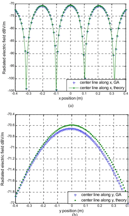
To test the operation of GA with the parameters defined above, the GA is used to find the polarization current on two identical dipoles of 3mm in size, placed 15cm apart. The radiated field is calculated using a full-field expression given in [6] with the dipole currents being in phase and set at 7.96 A at 2GHz. The cost function is the sum of the mean decibel errors of the three field components between the calculated radiated field and that calculated from the polarization currents found by the GA.
-0.4 -0.3 -0.2 -0.1 0 0.1 0.2 0.3 0.4 -105 -100 -95 -90 -85 -80 -75 -70
x position (m)
R ad ia te d el ect ric fie ld d B V /m
center line along x, GA center line along x, theory
-0.4 -0.3 -0.2 -0.1 0 0.1 0.2 0.3 0.4 -72 -71.8 -71.6 -71.4 -71.2 -71 -70.8 -70.6 -70.4
y position (m)
R ad ia te d el ect ric fie ld d B V /m
center line along y, GA center line along y, theory
Figure 3 Simulation result of fitting polarization current on dipoles using GA (a): H-plane cut, (b): E-plane cut
The error in the x-oriented field component is:
y y x x N n N
n GA mea
y x
x
N
N
E
E
C
1 1
{
log
10(
)
log
10(
)
}
20
(5)The overall error is therefore:
z y x
C
C
C
C
(6)WhereNxand Nyare the number of points along x and
y-axis on the observation surface. EGA and Emea represent the
radiated electric fields produced by the dipole moment from GA and that (measured or) calculated. The decibel value is
This work was partly funded under the EU Framework 7 programme contract number: 205294 (FP7) as part of the HIRF-SE project.
(a)
[image:3.595.327.551.165.539.2]taken to ensure that the curve fit is good for small field values as well as large ones.
The radiated field is taken on a planar surface 30cm from the dipole pair.Figure 3shows the calculated electric field and that reproduced using the excitation found by GA. Two plane cuts are shown here, where x is perpendicular to the direction of polarization, and y is parallel to the polarization direction
III. MEASUREMENTMETHOD
[image:4.595.36.279.169.328.2]A. Magnetic Field Probe
Figure 4 Loop antenna built as magnetic field probe
A magnetic field probe loop was fabricated on a microwave PCB laminate (Fig. 4). An outer loop with a gap acts as a shield against electric field pickup. Two rectangular copper plates are placed to provide further shielding against electric field on the loop side whilst a slotted ground-plane is used below the loop. The probe is terminated through two semi-rigid cables. One of those is mounted to an SMA connector, and another terminated by a 50 ohms load, which is formed by two 100 ohms surface-mount resistors, connected in parallel to reduce stray inductance.
1 2 3 4 5 6 7 8 9
-80 -75 -70 -65 -60 -55 -50 -45 -40 -35
Frequency (GHz)
S
21
(d
B
)
S21 Frequency Response of Loop with Copper Plate Shield
[image:4.595.321.545.176.415.2]0 degree cross-polar 180 degrees cross-polar 90 degrees co-polar 270 degrees co-polar
[image:4.595.309.533.450.643.2]Figure 5 Co-polar and cross-polar measurement of the loop in an anechoic chamber
Figure 5shows the co-polar and cross-polar measurement of the loop in an anechoic chamber. 0 degrees is defined as the direction of polarization of the incident electric field and is
parallel to the loop. It can be seen that the co-polar response is at least 10dB higher than that of the cross-polar response between 2GHz and 8.5GHz.
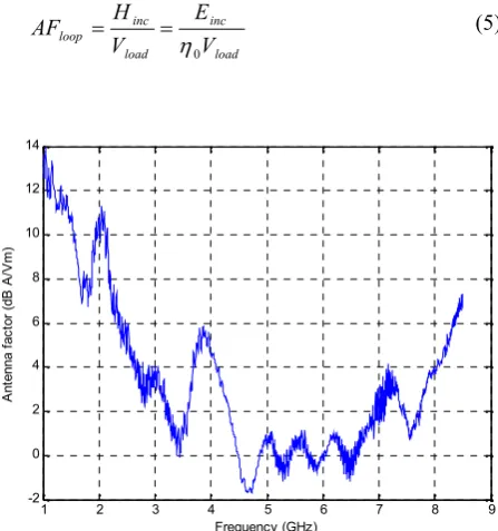
Since the loop is used to measure magnetic field, the antenna factor of the loop is defined as the ratio of incident magnetic field to load voltage. In the far-field region,
E
H
0, where 0is the impedance of free space. The antenna factor of the loop can then be written as:load inc
load inc
loop V
E V
H AF
0
(5)
1 2 3 4 5 6 7 8 9
-2 0 2 4 6 8 10 12 14
Frequency (GHz)
A
nt
en
na
fa
ct
or
(d
B
A
/V
m
)
Figure 6 Antenna factor of the loop
[image:4.595.64.278.464.647.2]B. Measurement Using Scaning Frame
Figure 7 Scanning fields penetrating the slot panel
Figure 8 Geometry of absorber box
[image:5.595.317.543.108.282.2]An absorber box [8] was used to produce an environment close to frees-pace by illuminating the sample being measured through a hole cut in absorbers. It saves time and cost on the edge treatment compared to a dual anechoic chamber measurement, and reduces the space required by the measurement facility.
Figure 9 TLM simulation of the slot array
[image:5.595.40.285.307.568.2]A TLM model of the slot structure was constructed to provide comparison with the measurement. The longitudinal magnetic field was recorded 13mm from the slot, which is the same as the measurement height inFigure 7.
Figure 11shows measurement result compared to that from the TLM simulation. The excitation in TLM was a plane wave of 1V/m z-polarized electric field, while that in the measurement was a horn antenna placed in a cavity surrounded
by absorber. The absolute magnetic fields cannot be compared, as the excitations are different.
0 20 40 60 80 100 120 140 160 180 200 -45
-40 -35 -30 -25 -20 -15
y position (mm)
R
at
io
o
f p
en
et
ra
tin
g
fie
ld
to
in
ci
de
nt
fi
el
d
(d
B
)
Measurement TLM simulation
Figure 10 Ratio of penetrating magnetic field to incident field in measurement and TLM simulation
IV. RESULTS
A. Use of the GA to fit measured near-field dipole moments
[image:5.595.308.549.425.570.2]In this section, the GA is used to reproduce the source using measurement data. The measurement was taken on the same slot array structure described Section III(b), which was also presented in a previous paper on this project [1].
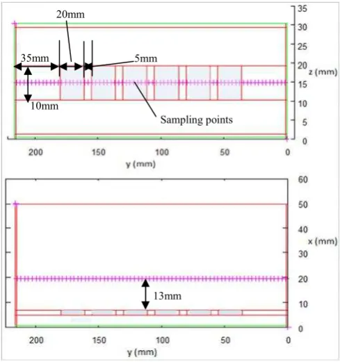
Figure 11 Equivalent magnetic dipoles of the slot array
Since only y-polarized electric field was measured, the cost function is modified so that the GA fits only Ey in the
measurement. The source is then constructed as 6 electric dipole moments, placed at the centers of the slots as shown in
Figure12.
The GA is set to run for 1000 generations, each with a population size of 50. Adaptive feasible is used as the mutation function. The results are plotted inFigures 13and14
below.
m1
m6 m2
m3 m4 m5
x
y 35mm
20mm
5mm
10mm
Sampling points
13mm Absorber
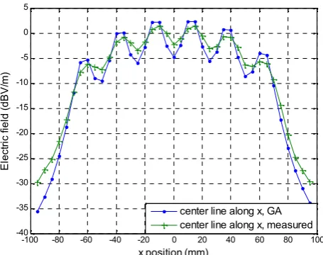
-100 -80 -60 -40 -20 0 20 40 60 80 100 -40
-35 -30 -25 -20 -15 -10 -5 0 5
x position (mm)
E
le
ct
ric
fie
ld
(d
B
V
/m
)
[image:6.595.49.277.63.243.2]center line along x, GA center line along x, measured
Figure 12 X-axis cut of electric field produced by GA and measurement
-100 -80 -60 -40 -20 0 20 40 60 80 100
-40 -35 -30 -25 -20 -15 -10 -5 0 5
y position (mm)
E
le
ct
ric
fie
ld
(d
B
V
/m
)
[image:6.595.49.279.277.455.2]center line along y, GA center line along y, measured
Figure 13 Y-axis cut of electric field produced by GA and measurement
Figure 13 and 14shows the dipole moments that the GA found can produce electric field follows the shape of that from measurement. In the measurement, the slots are so close that there is mutual coupling between them, which is not accounted in the field produced by the dipole moments. In addition, the measured field is averaged across the reception aperture of the measurement probe, while the field produced by the dipole moments is calculated at the exact location of the measuring point. It is considered the results can be improved
by increasing the density of the dipole moments and properly considering the averaging of the field produced by antenna physical size.
V. SUMMARY
In this paper, a GA has been shown to be capable of finding the magnitude of an equivalent radiating source based on simulation or measurement data. The specific goal of our modeling work is to reproduce the radiated field, so it is necessary to create an equivalent source that can produce a similar effect to the original source, rather than exactly re-creating the original source itself..
ACKNOWLEDGMENT
The authors would like to thank A White, A Patterson, J Emery, and M Hough, who fabricated the scanner hardware, and G Short who developed the scanner control and data acquisition software.
REFERENCES
[1] R. Xia, J. F. Dawson, I. D. Flintoft, A. C. Marvin and S. J. Porter, Building Marcro Models for Small Structures on Airframe , EMC Europe, 2011.
[2] D. M. Pozar, Microwave Engineering 2nd Edition . John Wiley & Sons, Inc.,1998. pp238.
[3] N. A. McDonald, Polynomial Approximations for the Transverse Magnetic Polarizabilities of Some Small Apertures, Microwave Theory and Techiniques, IEEE Transactions on, vol. 35, 1987, pp. 20-23. [4] N.A. McDonald, Simple Approximations for the Longitudinal
Magnetic Polarizabilities of Some Small Apertures, , Microwave Theory and Techiniques, IEEE Transactions on, vol. 36, 1988, pp. 1141-1144.
[5] C. A. Balanis, Antenna Theory, Analysis and Design 2nd Edition . John Wiley & Sons, Inc.,1997. pp135.
[6] J. D. Jackson, Classical Electromagnetics 3rd Edition , . John Wiley & Sons, Inc., 1999, pp411.
[7] Mathworks, Product R2012a Documentation: ga, available at: http://www.mathworks.co.uk/help/toolbox/gads/ga.html , Accessed 1 March 2012.
[8] A. C. Marvin, L. Dawson, I. D. Flintoft and J. F. Dawson, A Method for the Measurement of Shielding Effectiveness of Planar Samples Requiring no Sample Edge Preparation or Contact, IEEE Transactions on Electromagnetic Compatibility, Vol. 51, No. 2, April 2009.
Xia, R.; Dawson, J.F.; Flintoft, I.D.; Marvin, A.C.; Porter, S.J., "Use of a Genetic Algorithm in modelling small structures in airframes: Characterising and modelling joints, seams, and apertures," Electromagnetic Compatibility (EMC EUROPE), 2012 International Symposium on , vol., no., pp.1,5, 17-21 Sept. 2012
doi: 10.1109/EMCEurope.2012.6396718
![Figure 1 shows how the electric field penetrates an aperturein a conductive sheet. Providing the slot is electrically small,the penetrating field can be approximated by the fields ofelectric or magnetic dipoles placed on the surface of theconductive sheet [2].](https://thumb-us.123doks.com/thumbv2/123dok_us/7993963.206457/2.595.356.524.346.502/penetrates-aperturein-conductive-providing-electrically-penetrating-approximated-theconductive.webp)