A Straightforward Method for Wide-Area Fault Location on Transmission Networks

White Rose Research Online URL for this paper:

http://eprints.whiterose.ac.uk/143052/

Version: Accepted Version

Article:

Azizi, S orcid.org/0000-0002-9274-1177 and Sanaye-Pasand, M (2015) A Straightforward

Method for Wide-Area Fault Location on Transmission Networks. IEEE Transactions on

Power Delivery, 30 (1). pp. 264-272. ISSN 0885-8977

https://doi.org/10.1109/TPWRD.2014.2334471

© 2014 IEEE. Personal use of this material is permitted. Permission from IEEE must be

obtained for all other uses, in any current or future media, including reprinting/republishing

this material for advertising or promotional purposes, creating new collective works, for

resale or redistribution to servers or lists, or reuse of any copyrighted component of this

work in other works.

[email protected] https://eprints.whiterose.ac.uk/ Reuse

Items deposited in White Rose Research Online are protected by copyright, with all rights reserved unless indicated otherwise. They may be downloaded and/or printed for private study, or other acts as permitted by national copyright laws. The publisher or other rights holders may allow further reproduction and re-use of the full text version. This is indicated by the licence information on the White Rose Research Online record for the item.

Takedown

If you consider content in White Rose Research Online to be in breach of UK law, please notify us by

Abstract—Local practices in fault location require

mea-surements from one or more terminals of the faulted line to be available. On the other hand, the nonlinearity of circuit equations associated with wide-area fault location makes their solving process iterative and computationally demanding. This paper proposes a non-iterative method for wide-area fault location by taking advantage of the substitution theorem. Accordingly, a system of equations is constructed which can be easily solved using the linear least-squares method. The distributed-parameter line model is considered to provide a highly accurate estimation. Besides, due to inherent errors of current transformers, the current data is not taken into account to preserve the accuracy. In order to avoid uncertainties in relation with construction of zero-sequence network, just positive- and negative-sequence networks are exploited. Nonetheless, the method still is capable of pinpointing all types of short-circuit faults by using a restricted number of synchronized pre- and post-fault voltage phasors. Numerous simulation studies conducted on the WSCC 9-bus and New England 39-bus test systems verify the effectiveness and applicability of the proposed fault location method, even with limited coverage of synchronized measurements.

Index Terms—Phasor measurement unit (PMU), sequence

network, substitution theorem, wide-area fault location.

NOMENCLATURE

Ei,j Sum of squared residuals associated to the system of

equations, provided that line i-j is the faulted line. I Bus injected current vector.

I(i,j) _{Post-fault bus injected current vector, while line i-j}

has been replaced with equivalent current sources.

s f

I Fault path current in the sth sequence network. li,j Length of transmission line i-j.

s N

P Net power of the sth sequence network.

r N

P Net power of fault path. V Post-fault bus voltage vector.

s f

V Voltage of fault point f in the sth sequence network. Vpre _{Pre-fault bus voltage vector.}

Z Network impedance matrix.

Z(i,j) _{Network impedance matrix while line i-j has been}

removed.

This work was supported by the University of Tehran under Grant 8101064-1-07.

The authors are with the School of Electrical and Computer Engineering, College of Engineering, University of Tehran, Tehran 14395-515 Iran (e-mail: [email protected]; [email protected]).

,

c i j

Z Characteristic impedance of line i-j.

i,j Calculated fault distance on line i-j.

I. INTRODUCTION

RANSMISSION networks are always prone to various short-circuit faults along their lines. Fast and accurate fault location is required to improve the system reliability by reducing the outage and service restoration time. Accordingly, the problem of fault location has attracted a great deal of attention in the recent decades [1-17]. This problem has become more interesting since the emergence of new measurement and communication technologies [1-3].

Conventional fault location methods [4-12] necessitate one or more terminals of the faulted line to be equipped with measurement devices. Thus, if either of the measurement devices at the faulted line terminals fails to operate properly or is not in service during the fault, conventional methods would not be able to locate the fault [13]. Besides, some of these methods need the network model from the faulted line terminals, which should be regularly transmitted to the local substation from the dispatching center. On the other hand, fault location methods that utilize current data in their calculations are not immune to inherent errors of current transformers. This may considerably affect their accuracy.

Existing methods for wide-area fault location, as an application of wide-area monitoring system (WAMS), provide a good and viable solution for the fault location problem [2] and [13-17]. Meanwhile, they suffer from some technical difficulties such as need for iterative solution either by trial and error or by non-linear optimization techniques. Jiang et al. in[14] propose an algorithm to solve the nonlinear equations in relation to the wide-area fault location problem. This algorithm first determines the fault area using a voltage-based index and then locates the fault by a process of trial and error. A wide-area fault location scheme is presented in [15], which requires current and voltage phasors of at least one terminal of the faulted line. Furthermore, for this method to be applicable, a number of constraints over locations of phasor measurement units (PMUs) should be satisfied. The network impedance matrix along with the voltage measurements are deployed for wide-area fault location in [13]. This method, however, needs the faulted line to be pre-specified and can take advantage of only one or two different measurement devices at a time.

A Straightforward Method for Wide-Area Fault

Location on Transmission Networks

Sadegh Azizi, Student Member, IEEE, Majid Sanaye-Pasand, Senior Member, IEEE

of protective relays (PRs) and status of circuit breakers (CBs), provided that the main and backup protections are properly coordinated [18-20]. Nevertheless, such an approach becomes very complicated or even impossible after most power system blackouts, while the system is in an urgent need to be restored [21]. This is the case due to inclusion of data of mal-operated or failed PRs and CBs amongst the received data [22]. Therefore, it would be a great advantage for a fault location algorithm to be able to identify the faulted line, as well.

Practically speaking, it is difficult to obtain an accurate and reliable zero-sequence network. The reason is that the transmission line zero-sequence impedance is highly influenced by variable soil resistivity under the whole line route, and different weather conditions [26]. Accordingly, if possible, application of the zero-sequence network is better to be avoided in order not to deteriorate the fault location accuracy.

This paper proposes a novel wide-area fault location method by applying a limited number of synchronized voltage measurements across the network. The associated methodology is fully described in Sections II and III. In doing so, the substitution theorem is deployed to eliminate the iterative procedure involved in the existing wide-area fault location methods. The linear least-squares technique is then used to obtain the faulted line, its terminal voltages and either side injecting current. Although the zero-sequence network is not exploited due to its respective uncertainties, the proposed method is still capable of identifying all fault types. Moreover, the method successfully determines the faulted line as well as the fault distance on it, even in the case of limited WAMS coverage.

II. FAULT LOCATION ON SINGLE-PHASE NETWORKS In this section, the application of the substitution theorem in the normal operating condition is explained. Then, a technique based on the substitution theorem is developed to transform the fault location problem into an easier problem to be solved. Thus, the nonlinearity of formulations involved in the existing methods and required iterative solutions are eliminated.

A. Normal Operating Condition Equations

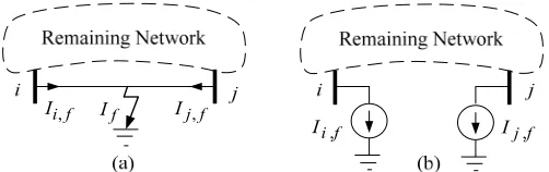
According to the substitution theorem, replacing a system component with a suitably adjusted current source injecting the same amount of current would change neither the system node voltages nor its branch currents. This property can be exploited to evaluate the network response while the equivalent network is easier to be solved than the original network [23]. Consequently, voltage and current phasors in the remaining networks of the original and equivalent networks shown in Figs. 1(a) and 1(b) would be identical.

For formation of a nodal equivalent network, every voltage source in series with its impedance should be converted to a suitable current source in parallel with that impedance, as discussed in [23], [24]. Accordingly, for the original single-phase network 1(a), the following equation can be written:

,  pre

V ZI (1)

where Z is the network impedance matrix in the normal operating conditionandVpreis the N×1 vector of pre-fault bus voltage phasors. Besides, I 





complex sum of all source currents entering bus k.

For the equivalent network 1(b), the relation between the injected currents and bus voltage phasors is as follows:

( )

1, , , , , , , ,

T

pre pre

i i j j j i N

I I I I I I

 

 _      _

pre i,j

V Z (2)

where Z(i,j) _{is the pre-fault network impedance matrix while}

the line i-j has been removed.

B. Faulted Branch Replacement

Assume in a single-phase network, voltages of buses 1 to m are measured. As shown in Fig. 2(a), a fault has occurred on the line i-j of the system. Based on the substitution theorem, the faulted line can be replaced with two equivalent current sources as depicted in Fig. 2(b). For the voltage and current phasors of the equivalent network 2(b), a matrix equation can be constructed as follows:

i,j i,j 

V Z( ) (I ), (3)

whereI( , )i j _I₁,,I_iI_{i f,} ,,I_jI_{j f,} ,I_N_T.

If the substituted line i-j is actually the faulted line, the topology of the rest of network would be the same as that of the pre-fault network, independent of the fault distance along the line i-j. Consequently, Z(i,j) _{having been constructed based}

on the pre-fault network topology would be still valid for calculation purposes under the fault condition. This is the key idea to get rid of the nonlinear impedance matrix as a function of the exact fault location on the faulted line.

,

i j

I I_{j i,}

,

pre i j

I I_{j i}pre_,

Fig. 1. Response equivalency between (a) the original and (b) equivalent branch-replaced single-phase networks under the normal operating condition.

,

i f

I I_{j f,}

,

i f

I I_f I_{j f,}

Let the symbol be used to denote the change in a variable due to the fault, i.e., the difference between its pre- and post-fault values. It can be concluded from (2) and (3) that:

( , ) ( , ) 1, 1, 1 , , ( , ) ( , ) , , . i j i j j i i j j i

i j i j

m

m i m j

Z Z

V

I I

V _{Z Z}

     _{   }  _{    }   _{   }     _{ }   _{ }

   (4)

whereI_i,j I_{i f,} I_ipre_,j and I_j,i I_{j f,} Ipre_j,i are the unknowns. The reason for the negative sign on the right hand side of (4) is because the current sources whose reference directions exit the connected terminal have been assigned a negative sign in (2) and (3).

The system of linear equations (4) is an over-determined system of equations having no solution in general. Nevertheless, it can be solved using the linear least-squares method to specify the values of the best two fitting current sources for each suspected line. Such a solution ensures that the sum of squared residuals is minimal, where a residual is defined as the difference between the measurement and its fitted value provided by the respective equation in (4).

With the assumption that the line i-j is faulted and after calculation of Ii,j and Ij,i, the sum of squared residuals of (4)

is derived as:





( , ) ( , )

, , , , ,

1

m

i j i j

i j k k i i j k j j i

k

E V Z I Z I



 

 _     _

 



It should be pointed out that the actual faulted line and the respective fault distance on it are the unknowns for which (4) is definitely satisfied. It means that Ei,j takes a very small

value for the faulted line. Thus, the faulted line can be specified by comparing the calculated Ei,j’s for examined

transmission lines, since the smallest one corresponds to it. Having calculated Ii,j and Ij,i from (4), Vi and Vj can

be determined using (2) and (3) as: ( , ) ( , )

, , ,

( , ) ( , ) _,

, ,

.

i j i j

i i i j i j

i

i j i j

j j i

j i j j

Z Z I V

V _{Z Z} I

 _{  }    _{ }     _  _{  }  

  _{ }  (6)

Assume the characteristic impedance of the faulted line, say the line i-j, is denoted by Z_{i, j}c and its propagation constant is equal to i,j. Let i,j= i,j×li,j where li,j is the line length. The

closed form expression for the fault distance _{i j,} is derived by equating the KVL equations written from both ends of the faulted line to the fault point, as follows [25]:

, , , , , , 1 , , , , , , 1 (7)

cosh( ) sinh( )

tgh

sinh( ) cosh( )

i j i j

c

i j j i j i j j i i

c c

i j j i j i j j i i j i j

V Z I V

V Z I Z I

          _{    }     _{    }   

III. FAULT LOCATION ON TRANSMISSION NETWORKS Following a fault, voltage and current phasors at different

network buses and branches vary with respect to the fault type, location and resistance. Symmetrical components method transforms the solution of an unbalanced three-phase network into the solution of three balanced sequence networks [24]. Interconnection of these networks so as to satisfy the fault type constraints yields an integrated circuit to be solved. Meanwhile, according to the substitution theorem, each sequence network can be analyzed separately by replacing the remaining networks with a suitable current source. In the proposed method, only the positive- and negative-sequence networks are deployed to determine the fault type, faulted line and fault distance on it.

A. Faulted Line Identification

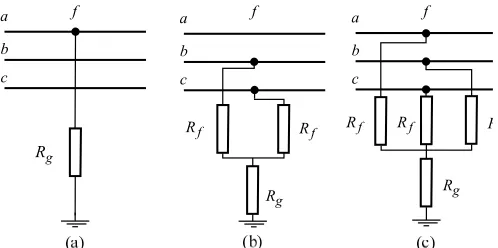
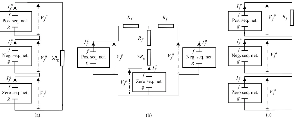
Figs. 3(a), 3(b) and 3(c) depict the basic models of various fault types as considered in most fault-location algorithms. These models represent single-phase-to-ground (1-ph-g), two-phase-to-ground (2-ph-g), and three-two-phase-to-ground (3-ph-g) faults, respectively. It should be noted that 2-ph and 3-ph faults can be considered as particular cases of 2-ph-g and 3-ph-g faults while Rg is infinite. The proper interconnections of

the sequence networks corresponding to these fault types are illustrated in Figs. 4(a), 4(b) and 4(c), respectively. Besides, a proof for such interconnection in the general case of 2-ph-g fault, i.e., Fig. 4(b), is provided in Appendix.

Owing to symmetry, the negative-sequence voltages and currents all over the network are quite negligible for a 3-ph-g fault [26]. Thus, if PMUs observe no negative-sequence quantities during the fault, it implies that a symmetrical fault is encountered. In such a case, it is only required to pinpoint the fault on the positive-sequence network. The procedure would be exactly similar to the one explained in the previous section for the single-phase networks.

The both of positive- and negative-sequence networks should be analyzed in the case of asymmetrical faults. According to the substitution theorem, each of these two networks can be treated as a single-phase network. Similarly, the faulted line can be replaced with two suitably adjusted current sources so that the response of the associated remaining network is unaffected. As such, all variables, matrices and parameters in (1)-(7) can be labeled with the superscripts “s” representing them in the sth sequence network. Accordingly, I_{i , j}s , Is_{j ,i},V_is,V_js and _{i j}s_, can be obtained for each sequence network, independently.

f a b c f a b c f a b c g R f

R R_f Rf Rf R

g

R Rg

Consider Fig. 5 which illustrates the faulted line i-j in the sth sequence network. The superscript “s” can take values of “z”, “p” and “n” for zero-, positive-, and negative-sequence networks, respectively. If the ABCD parameters of

, ,

s i j i jl

 and(1_{i j}s_, )l_{i j,} portions of the faulted transmission line are calculated based on [24], the voltage dropped across the fault path, and fault path current can be derived as:

, , , , , ,

cosh( ) sinh( ) ,

s s s c s s

f i j i j i i j i j i j i f

V    V Z   I (8)

, , , , , ,

, , , ,

, ,

cosh( ) cosh((1 ) )

1 1

sinh( ) sinh((1 ) ) .

s s s s s

f i j i j i f i j i j j f

s s s s

i j i j i i j i j j

c c

i j i j

I I I

V V

Z Z

    

    

   

    (9)

To obtain V_fsand I_fs, every signal in (8) and (9) should be replaced with its pre- and post-fault difference, which can be readily calculated from (4) and (6). On the other hand,

s f

I

 =I_fswhich means the fault path current can be obtained independent of the pre-fault signals of the faulted line.

The methodology presented in Section II can be exploited to pinpoint the fault distance on the line i-j in the positive- and negative-sequence networks. Let the calculated fault distances on the line i-j in the positive- and negative-sequence networks be _{i j}p_, and _{i j}n_, , respectively. If the line i-j is actually the

faulted line, the following constraint must be satisfied:

, ,

0i jp i jn 1. (10)

Constraint (10) is the first constraint that has to be checked for determining whether or not the examined line is the faulted line.

Let P_Nz ,P_Np,P_Nn and P_Nr be the net power of the zero-, positive- and negative-sequence networks, and the fault path, respectively. On the basis of the energy conservation law, it can be concluded that:

0

p

z n r

N N N N

P P P P  . (11)

The fault path is passive and mainly demonstrates resistive characteristics [26]. Thus, the equivalentP_Nr resulting from the faulted line replacement with current sources must be negative and can be utilized as a constraint to identify the faulted line. However, this constraint cannot be directly checked since the fault path resistance is not known. If the pre-fault state of the faulted line, and hence the pre-fault voltage of the fault point is available, passivity of the fault path can be identified from (11). Nonetheless, it is intended in this paper not to use the zero-sequence quantities. Therefore, another proper constraint would be used as an alternative.

Zero- and negative-sequence networks are passive similar to the fault path, and their net generated powers are negative. Mathematically speaking,

0,

r N

P  (12)





=Real ( ) 0,

z z z

N f f

P V  I  (13)





=Real ( ) 0.

n n n

N f f

P V  I  (14)

Since P_Np  (P_Nz P_Nn P_Nr)and P_Nz ,P_Nn and P_Nr are all negative, it follows that:





Real ( ) 0.

p p p

N f f

P  V  I  (15)

Pos. seq. net.

f g

Neg. seq. net.

f g

Pos. seq. net.

f g

z f

I

Zero seq. net.

f g

Neg. seq. net.

f

g 3Rg

Pos. seq. net.

f g

z f

I

Zero seq. net.

f g

z f

V

Neg. seq. net.

f g f R z f V f R f

R R_f

3Rg z f

I

Zero seq. net.

f g n f I z f V n f V p f V p f

V Vfn

n f

I

p f

I Ifn

n f V p f V

Fig. 4. Sequence networks interconnection corresponding to (a) single-phase-to-ground, (b) two-phase-to-ground, and (c) three-phase-to-ground faults.

,

s i f

I Is_{j f,}

s f

I

s i

V _s Vs_j

i, j i, jl

 (1 _{i, j i, j}s )l

s f

V

By rearranging equation (11), it is obtained that

( ).

p n z r

N N N

N

P P   P P With respect to (12) and (13), P_Nz

and P_Nr are both negative, which means their sum is negative as well. It directly follows that:

P_NpP_Nn Real





Now, it is possible to express (14)-(16) as a single inequality constraint as:

0P_Np P_Nn P_Np (17)

To summarize, the negativeness of P_Nr could be directly checked, if the zero-sequence network model would be accurate enough. Not using the zero-sequence quantities, constraint (17) should be satisfied as a necessary condition for

r N

P to be negative.

B. Fault Location Algorithm

Based on the formulations derived in Sections II and III-A, a systematic algorithm is presented in this part for wide-area fault location. In fact, the suitable equations proposed in the previous sections are used to transform the problem into a regular two-terminal fault location problem. This is possible with the assumption that the network positive- and negative-sequence impedance matrices are constructible thanks to the SCADA or WAMS. Additionally, the pre- and post-fault voltage measurements at a limited number of buses, i.e., buses 1 to m, are utilized.

Upon a short-circuit fault, every transmission line should be examined to specify if it is faulted. This could be achieved by replacing the line with two current sources in either of the sequence networks as described earlier. Meanwhile, this procedure can be limited only to the suspected transmission lines to further reduce the computational burden. For the actual faulted line, the calculated _{i j}p_, and _{i j}n_, would be equal and lie between 0 and 1, which is evaluated by constraint (10). The passivity of the fault path can be also checked using (17).

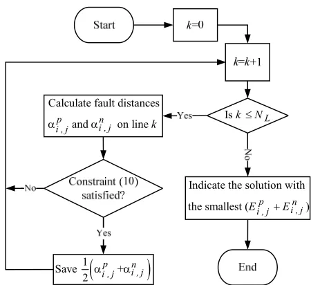
The flowchart of the proposed fault location method is depicted in Fig. 6. As shown, the fault location process is pursued for all NL transmission lines in the network. It is quite

reasonable to expect that the obtained fault distance for healthy transmission lines lies out of the acceptable range or is not even a real number. However, in some rare cases, the estimated fault distance for a healthy line might be a real number in the range [0,1]. This is more likely to happen for adjacent lines to the faulted line. In such a condition, the sum of squared residuals is checked to indicate the faulted line. The reason is because the sum of squared residuals of the system of equations (4), i.e., Ei,j, would be ideally equal to zero if the

line replaced with the current sources is the faulted one. Consequently, the fault location algorithm based on the proposed methodology can be described as follows:

I. For the transmission line i-j, solve (4) for the sth sequence

network to obtainI_{i f}s_, andIs_{j f,} using the least-squares method.

II. Use (6) to calculate V_isandV_js.

III. For the positive- and negative-sequence networks, use (7) to obtain the fault distances _{i j}p_, and _{i j}n_, on the line i-j.

IV. Save 1





2

p n

i j i j

  and the associated Ei,j as a feasible

solution for cases where (10) is satisfied.

V. Indicate the feasible solution with the minimum sum of squared residuals as the fault location result.

C. Fault Type Identification

By using the proposed method, not only the faulted line and fault location are successfully determined, but also the fault type can be identified. To explain this feature of the proposed method, assume the fault location has been accurately pinpointed as described beforehand. Now, the fault path current can be calculated using (10). As a result, the fault type can be readily identified by investigating the current flowing through the fault path. To do so, it is only needed to compare the fault currents in positive- and negative- sequence networks.

To clarify, assume a short-circuit fault has occurred in the system. If the negative voltage phasors measured at PMU locations, i.e., V₁n, V₂n, …, V_mn, are very small, it can be inferred that the fault is a symmetrical fault. In such a case, only the positive-sequence network is required to be analyzed to find the fault distance _{i j}p_, . However, the both of positive

and negative signals change during asymmetrical faults. In such cases, the calculated fault locations using the positive- and negative-sequence networks must be the same. It follows from the sequence networks interconnection that for 1-ph-g faultsI_fp I_fn. Conversely, for 2-ph-g faults I_fn I_fp. In the

Calculate fault distances

and on line

p n

i , j

i , j k

  IskNL

Indicate the solution with

the smallest (E_{i , j}p E_{i , j}n )





1 Save +

2

p n

i , j i , j

 

special case of 2-ph faults where Rg=0, I_fp  I_fn. Therefore,

in spite of circumventing the zero-sequence network, it is still possible to pinpoint the fault location and its type using the proposed method.

IV. SIMULATION RESULTS

To demonstrate the effectiveness of the proposed wide-area fault location method, the WSCC 9-bus and New England 39-bus test systems [27] are studied in this section. The 9-39-bus test system consists of 6 transmission lines, 3 transformers and 3 generation units. Besides, this system is equipped with 2 PMUs at buses 6 and 9. On the other hand, the 39-bus test system consists of 34 transmission lines, 12 transformers and 10 generation units. Moreover, similar to [28], 8 PMUs are installed in this system. The single line diagrams of these two test systems are shown in Figs. 7 and 8, respectively.

In this paper, DIgSILENT Power Factory software is

deployed as the power system simulator [29]. All generated signals are then passed through a second-order Butterworth anti-aliasing filter with a cut-off frequency of 400 Hz. The filtered signals are sampled with a sampling rate of 2400 Hz, i.e., 48 samples per cycle. The discrete Fourier transform (DFT) is exploited to extract the fundamental-frequency component of the obtained signals. The measured voltage signals during the fault interval, starting from the fault inception until the circuit-breaker operation, can be fed to the proposed method to calculate the fault distance at every time instant. In this paper, the estimated fault distance is averaged from 30 ms to 60 ms after the fault inception time to obtain more reliable results. Besides, to demonstrate the fault location accuracy, the relative difference between the actual and estimated fault location is calculated as follows:

Estimated FL - Actual FL

Estimation Error(%) 100.

Faulted Line Length

  (18)

A. WSCC 9-Bus Test System

In this part, the applicability of the proposed method is examined on the 9-bus test system. The method is also evaluated for high impedance faults with transient contents. 1) General evaluation of proposed fault location method

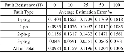
In the 9-bus test system, all fault types have been simulated at five points on every transmission line, i.e., 10%, 30%, 50%, 70% and 90% of the line length. Various amounts of fault resistance from 0 to 100 are examined to study its effect on the fault location accuracy. Considering all these locations, examined fault types and different amounts of fault resistance, a total of 600 case studies are simulated. Table I summarizes the obtained results for 1-ph-g, 2-ph, 2-ph-g and 3-ph-g faults, and all of them in total. In general, the estimation accuracy declines when the fault resistance increases. Besides, the average estimation error does not exceed 0.2% in any case, regardless of the fault type, location and resistance.

To illustrate that the proposed method can effectively pinpoint the fault location and its type without using the zero-sequence quantities, a series of simulation results are tabulated in Table II. These results correspond to the simulation of four different fault types with 100 resistance, at distance 40 % of line 7-8. All quantities in this table except its last two rows, are calculated only by using the positive- and negative-sequence voltage phasors at PMU buses 6 and 9. Meanwhile, the last two rows of the table is calculated given the pre-fault

FAULT LOCATION RESULTS ON 9-BUS TEST SYSTEM

Fault Resistance ( ) 0 10 25 50 100

Fault Type Average Estimation Error %

1-ph-g 0.1404 0.1653 0.1709 0.1769 0.1818

2-ph 0.0935 0.1076 0.1092 0.1017 0.1085 2-ph-g 0.1156 0.1317 0.1432 0.1471 0.1561

3-ph-g 0.044 0.0591 0.0551 0.0566 0.0761 All in Total 0.0984 0.1159 0.1196 0.1204 0.1306

voltage at the fault point is 0.991 0.0321 . The seventh row of the table demonstrates based on which constraint the fault type has been identified. It can be inferred from the table that although the method does not take into account the zero-sequence quantities, it is still capable of fault type identification.

2) Nonlinear high impedance faults

To model the time-varying arc resistance, its dynamic volt-ampere characteristics are taken into account based on the empirical differential equation described in [26]. Then, this arc model in series with a 100 resistance is used to evaluate the proposed method performance for nonlinear high impedance faults. In doing so, various distances on the line 7-8 of the 9-bus test system are examined for 1-ph-g faults. The obtained results are summarized in Table III. It can be observed that the involvement of a nonlinear high impedance fault reduces the fault location accuracy. However, the obtained results would be still acceptable from a practical point of view.

B. New England 39-Bus Test System

In this part, the applicability of the proposed method is examined on the New England 39-bus test system. Fault location on this system is first carried out using the set of PMUs shown in Fig. 8. Then, the influence of limited WAMS coverage and other factors is investigated.

1) General evaluation of proposed fault location method Table IV summarizes the results of more than 3000 simulated fault cases on this test system. As before, five points on every transmission line are examined. As tabulated in Table IV, fault location is successfully carried out for the simulated cases, with high precision. The average estimation error does not exceed 0.25% in any case, regardless of the fault type, location and resistance. Based on the results, it can be also concluded that the estimation accuracy declines slightly as the fault resistance increases. However, the maximum estimation error hardly exceeds 0.5% even for large resistance values. Practically speaking, this amount of error is quite negligible.

2) Estimation accuracy along a transmission line

To examine how the estimation accuracy is affected by the fault distance on the transmission line, a number of 1-ph-g faults are simulated at various locations on the line 13-14 of the 39-bus test system. This line is selected since none of its terminals is PMU-equipped or even observed with an installed PMU at an adjacent bus. The obtained results are used to calculate the percentage estimation error based on (18). To be useful, the estimation accuracy versus the fault distance on the line 13-14 is depicted in Fig. 9. As shown, the estimation error does not exceed 0.25% along the line. Further simulations conducted by the authors show that the method accuracy is not noticeably affected by change in the fault inception time or the pre-fault machine phase angles.

3) Fault location with limited WAMS coverage

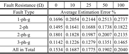
The network observability is not a necessary condition for wide-area fault location [13], [14]. Theoretically speaking, even two synchronized voltage measurements suffice for (4) to be solvable and hence, to locate the fault using the proposed method. However, in practice, the more the number of PMUs is, the better the fault location result would become. To investigate the fault location accuracy with limited WAMS coverage, a PMU set is considered at buses 11, 20, 23, 25 and 29 of the 39-bus test system. Table V shows the summary of fault location for more than 3000 simulated cases using this new set of PMUs. As can be seen, the method successfully

TABLE II

FAULT TYPE IDENTIFICATION FOR FAULTS AT DISTANCE 40% OF LINE 7-8

Fault Type 1-ph-g 2-ph 2-ph-g 3-ph-g

, (%)

p i j

 0.3978 0.4014 0.4003 0.4004

, (%)

n i j

 0.3995 0.4016 0.4027 ---

(pu)

p p

f f

I I

  _-j0.6068 1.0533 _-j1.8136 2.0811 _-j1.1416 2.1739 _-j1.61953.3705

(pu)

n n

f f

I I

  _-j0.6084 1.0534 _+j1.8141 -2.0809 _+j0.4804 -1.1982 0.000

(pu)

p f

V

 -0.1041

-j0.1115

-0.2807 -j0.203

-0.2012 -j0.2334

-0.2936 -j0.3661

(pu)

n f

V

 _-j0.1115 -0.1043 _+j0.2029 0.2807 _+j0.1328 0.0927 0.000

Satisfied Constraint

p n

f f

I I Ifp Ifn

p n

f f

I I V_fnI_fn0 Identified Fault

Type 1-ph-g 2-ph 2-ph-g 3-ph-g

(pu)

p N

P 0.982 1.787 1.946 2.890 (pu)

n N

P -0.042 -0.216 -0.047   0.000

TABLE IV

FAULT LOCATION RESULTS ON 39-BUS TEST SYSTEM

Fault Resistance ( ) 0 10 25 50 100

Fault Type Average Estimation Error % 1-ph-g 0.1493 0.1667 0.1754 0.1915 0.2243

2-ph 0.1156 0.1218 0.1173 0.1194 0.1248

2-ph-g 0.1457 0.1499 0.1572 0.1501 0.1631

3-ph-g 0.0782 0.0764 0.0791 0.0807 0.0862 All in Total 0.1222 0.1287 0.1322 0.1354 0.1496

0.1 0.2 0.3 0.4 0.5 0.6 0.7 0.8 0.9 0

0.05 0.1 0.15 0.2 0.25

Distance (%)

E

st

im

at

io

n

E

rro

r (%

) Possitive-Sequence Negative-Sequence Average

Fig. 9. Estimation error for faults at different distances on the line 13-14.

TABLE III

FAULT LOCATION FOR NONLINEAR HIGH IMPEDANCE FAULTS ON LINE 7-8

Actual Fault Distance % 10 30 50 70 90

locates short-circuit faults with an average error of less than 0.3%, even for high-impedance faults. It can be concluded that the estimation accuracy has slightly decreased due to the limited WAMS coverage.

4) Effect of synchronization error on estimation accuracy Synchrophasor measurements must be synchronized with a maximum time error of ±31 s for a 50 Hz system, to meet the accuracy requirements of the IEEE standard [30]. In order to test the proposed scheme with synchronization errors that might occur due to different technical problems, an exaggerated time error of ±56 s, corresponding to a phase error of ±1°, is considered for measurements. This amount of error is assumed to have a normal distribution with mean zero. Fig. 10 depicts the obtained results for a total of 1000 1-ph-g fault cases at 70% of the line 1-39. As depicted, the estimated fault distances demonstrate a normal distribution with mean and standard deviation of 70.26% and 0.083 %, respectively.

V. CONCLUSIONS

A novel method was proposed in this paper for wide-area fault location on transmission networks. It was shown that the substitution theorem can be deployed in a way that the network impedance matrix constructed based on the pre-fault network topology is still valid for calculation purposes under the fault condition. Hence, despite the nonlinearity involved in the associated equations to wide-area fault location, the fault distance would be accurately determined using the linear least-squares method. On the other hand, taking into account the shunt capacitance of transmission lines does not affect the linearity of the proposed method.

Overall, the major achievements of the proposed method can be summarized as follows:

 A limited number of pre- and post-fault voltage phasors just for few cycles are sufficient to accurately determine the fault location.

 The proposed method rigorously specifies the faulted line while not requiring it as an input.

 High computational burden and algorithm failure in finding the optimal solution are totally eliminated using the linear least-squares method.

 Although the zero-sequence network is not exploited due to the related uncertainties, the fault type would be identified, as well.

 Current data is not utilized due to accuracy concerns.

 Obtained result is quite accurate even for large amounts of fault resistance.

APPENDIX

In Fig. 3(b), a basic fault model has been considered for the general case of two-phase faults involving ground as described in [26]. It is intended to obtain an equivalent model for this type of fault in sequence domain, by suitable interconnection of the sequence networks. The associated fault conditions in phase domain can be expressed as:

( )

.

( )

b b b c

f f f g f f

c c b c

f f f g f f

V R I R I I V R I R I I

 _{  }

 

  

 (A-1)

Summation and subtraction of these two equations provide:





2 ( )

b c b c

f f f f f

b c b c

f f f g f f

V V R I I

V V R R I I

 _{  }

 

   

 (A-2)

Since the current of the non-faulted phase is zero, we have:

0.

p

a n z

f f f f

I I I I  (A-3)

Besides, using the approach introduced in [24], it is possible to express equations of (A-2) in the sequence domain as:





p n p n

f f f

f f

V V R I I (A-4)









2V_fz V_fp V_fn 3 R_f 2R_g I_fz. (A-5) After some algebraic manipulations on (A-5), and utilizing

(A-3) and (A-4), the following equations can be derived:

3

3

p p z z z

f f f f g f

f f

n n z z z

f f f f f f g f

V R I V R I R I V R I V R I R I

 _{   }

 

   

 (A-6)

The equations (A-3), (A-4) and (A-6) altogether represent the fault conditions, in sequence domain. To always satisfy (A-3), the three sequence networks should be terminated in a common node. Besides, Rf should be included in series with

either of positive- and negative-sequence networks to satisfy (A-4). Finally, if Rf as well as 3Rg are added in series with the

zero-sequence network, equations in (A-6) are guaranteed to hold true. Accordingly, the equivalent model for two-phase faults involving ground would be as shown in Fig. 4(b).

REFERENCES

[1] M. Kezunovic, “Smart fault location for smart grids,” IEEE Trans. Smart Grid, vol. 2, no. 1, pp. 11-22, Mar. 2011.

Fault Resistance ( ) 0 10 25 50 100

Fault Type Average Estimation Error % 1-ph-g 0.1696 0.2054 0.2144 0.2513 0.2737

2-ph 0.1495 0.1641 0.1688 0.1738 0.1822

2-ph-g 0.1801 0.1828 0.1987 0.2007 0.2135

3-ph-g 0.1142 0.1226 0.1279 0.1351 0.1465

All in Total 0.1534 0.1687 0.1775 0.1902 0.2040

69.9 70 70.1 70.2 70.3 70.4 70.5 70.6 70.7 0

20 40 60 80 100 120 140

Estimated Fault Distance %

N

o

. o

f Ca

se

s

[2] A. S. Dobakhshari, and A. M. Ranjbar, “Application of synchronised phasor measurements to wide-area fault diagnosis and location,” IET Generation, Transmission & Distribution., vol. 8, no. 4, pp. 716-729, Sep. 2014.

[3] M. Korkali, H. Lev-Ari, and A. Abur, “Traveling-wave-based fault location technique for transmission grids via wide-area synchronized voltage measurements,” IEEE Trans. Power Syst., vol. 27, no. 2, pp. 1003-1011, May 2012.

[4] K. Takagi, Y. Yomakoshi, M. Yamaura, R. Kondow, and T. Matsushima, “Development of a new type fault locator using the one-terminal voltage and current data,” IEEE Trans. Power App. Syst., vol. PAS-101, no. 8, pp. 2892–2898, Aug. 1982.

[5] J. Izykowski, E. Rosolowski, M. M. Saha, “Locating faults in parallel transmission lines under availability of complete measurements at one end”, in Proc. Inst. Elect. Eng., Gen., Transm. Distrib., vol. 151, no.2, pp. 268–273, Mar. 2004.

[6] A. M. Ranjbar, A. R. Shirani, and A. F. Fathi, “A new approach for fault location problem on power lines,” IEEE Trans. Power Del., vol. 7, no. 1, pp. 146–151, Jan. 1992.

[7] S. M. Brahma and A. Girgis, “Fault location on a transmission line using synchronized voltage measurements,” IEEE Trans. Power Del., vol. 19, no. 4, pp. 1619–1622, Oct. 2004.

[8] Y. H. Lin, C. W. Liu, and C. S. Chen, “A new PMU-based fault detection/location technique for transmission lines with consideration of arcing fault discrimination—Part I: Theory and algorithms,” IEEE Trans. Power Del., vol. 19, no. 4, pp. 1587–1593, Oct. 2004.

[9] I. Zamora, J. F. Minambres, A. J. Mazon, R. Alvarez-Isasi and J. Lazaro, “Fault location on two-terminal transmission lines based on voltages”, in Proc. Inst. Elect. Eng., Gen., Transm. Distrib., vol. 143, no. 1, pp. 1–6, Jan. 1996.

[10] M. Abe, T. Emura, N. Otsuzuki, and M. Takeuchi, “Development of a new fault location system for multi-terminal single transmission lines,” IEEE Trans. Power Del., vol. 10, no. 1, pp. 159–168, Jan. 1995. [11] S. M. Brahma, “Fault location scheme for a multi-terminal transmission

line using synchronized voltage measurements,” IEEE Trans. Power Del., vol. 20, no. 2, pt. 2, pp. 1325–1331, Apr. 2005.

[12] J. Izykowski, E. Rosolowski, M. M. Saha, M. Fulczyk, and P. Balcerek, “A fault-location method for application with current differential relays of three-terminal lines,” IEEE Trans. Power Del., vol. 22, no. 4, pp. 2099–2106, Oct. 2007.

[13] Y. Liao, “Fault location for single-circuit line based on bus-impedance matrix utilizing voltage measurements,” IEEE Trans. Power Del., vol. 23, no. 2, pp. 609–617, Apr. 2008.

[14] Q. Jiang, X. Li, B. Wang, and H. Wang, “PMU-based fault location using voltage measurements in large transmission networks,” IEEE Trans. Power Del., vol. 27, no. 3, pp. 1644–1652, Jul. 2012.

[15] K. P. Lien, C. W. Liu, C. S. Yu, and J. A. Jiang, “Transmission network fault location observability with minimal PMU placement,”IEEE Trans. Power Del., vol. 21, no. 3, pp. 1128-1136, Jul. 2006.

[16] M. Kezunovic and Y. Liao, “Fault location estimation based on matching the simulated and recorded waveforms using genetic algorithms,” in Proc. Int. Conf. Develop. Power Syst. Protect., RAI, Amsterdam, the Netherlands, Apr. 2001.

[17] A. S. Dobakhshari, and A. M. Ranjbar, “A circuit approach to fault diagnosis in power systems by wide-area measurement system,” International Transactions on Electrical Energy Systems., vol. 23, no. 8, pp. 1272–1288, Nov. 2013.

[18] G. Cardoso, J. G. Rolim, and H. H. Zurn, “Identifying the primary fault section after contingencies in bulk power systems,” IEEE Trans. Power Del., vol. 23, no. 3, pp. 1335–1342, Jul. 2008.

[19] R. N. Mahanty and P. B. D. Gupta, “Application of RBF neural network to fault classification and location in transmission lines,” in Proc. Inst. Elect. Eng., Gen., Transm. Distrib., vol. 151, no. 2, pp. 201–212, Mar. 2004.

[20] L. Xu and M. Kezunovic, “Implementing fuzzy reasoning Petri-nets for fault section estimation,” IEEE Trans. Power Del., vol. 23, no. 2, pp. 676–685, Apr. 2008.

[21] S. A. N. Sarmadi, A. Salehi Dobakhshari, S. Azizi and A. M. Ranjbar, “A sectionalizing method in power system restoration based on WAMS,” IEEE Trans. Smart Grid, vol. 2, no. 1, pp. 190-197, March 2011.

[22] D. Novosel, G. Bartok, G. Henneberg, P. Mysore, D. Tziouvaras, and S. Wasrd, “IEEE PSRC report on performance of relaying during wide-area stressed conditions,” IEEE Trans. Power Del., vol. 25, no. 1, pp. 3– 16, Jan. 2010.

[23] Desoer and E. S. Kuh, Basic Circuit Theory, New Delhi: Tata McGraw-Hill, 2009.

[24] H. Saadat, Power System Analysis, 2nd ed., New York: McGraw-Hill, 2002.

[25] A.T. Johns, S. Jamali, “Accurate fault location technique for power transmission lines,” in Proc. IEE Gen., Transm. Distrib., vol. 137, no. 6, pp. 395–402, Nov. 1990.

[26] M. M. Saha, J. J. Izykowski, and E. Rosolowski, Fault Location on Power Networks, 1st ed. Springer: London, 2010.

[27] [Online]. Available: http://www.pserc.cornell.edu/matpower/.

[28] F. Aminifar, A. Khodaei, M. Fotuhi-Firuzabad, M. Shahidehpour, “Contingency-constrained PMU placement in power networks,” IEEE Trans. Power Syst., vol. 25, no. 1, pp. 516 – 523,Feb. 2010.

[29] DIgSILENT GmbH: ‘DIgSILENT Power Factory, Version 14’, 2008. [30] IEEE Standard for Synchrophasors for Power Systems, IEEE Standard

C37.118-2005, Mar. 2006.

[31] A. Abur, and A. G. Exposito, Power System State Estimation: Theory and Implementation, Marcel Dekker, Inc. 2004.

Sadegh Azizi (S’12) received the B.Sc. degree in electrical engineering from K. N. Toosi University of Technology, Tehran, Iran, in 2007, and the M.Sc. degree in the same field from Sharif University of Technology, Tehran, Iran, in 2010. He is currently pursuing the Ph.D. degree in electrical engineering at the University of Tehran, Tehran, Iran.

His research interests include applications of wide-area monitoring, protection and control system, digital protective relays, and power system stability studies.

Majid Sanaye-Pasand (M’98–SM’05) received the electrical engineering degree from the University of Tehran, Tehran, Iran, in 1988, and the M.Sc. and Ph.D. degrees in electrical engineering from the University of Calgary, Calgary, AB, Canada, in 1994 and 1998, respectively.