This is a repository copy of Impulsively-controlled systems and reverse dwell time: A linear programming approach.
White Rose Research Online URL for this paper: http://eprints.whiterose.ac.uk/89653/
Version: Accepted Version
Article:
Bauso, D. (2015) Impulsively-controlled systems and reverse dwell time: A linear
programming approach. Nonlinear Analysis: Hybrid Systems, 16. 40 - 51. ISSN 1751-570X https://doi.org/10.1016/j.nahs.2014.11.004
Reuse
Unless indicated otherwise, fulltext items are protected by copyright with all rights reserved. The copyright exception in section 29 of the Copyright, Designs and Patents Act 1988 allows the making of a single copy solely for the purpose of non-commercial research or private study within the limits of fair dealing. The publisher or other rights-holder may allow further reproduction and re-use of this version - refer to the White Rose Research Online record for this item. Where records identify the publisher as the copyright holder, users can verify any specific terms of use on the publisher’s website.
Takedown
If you consider content in White Rose Research Online to be in breach of UK law, please notify us by
Impulsively-controlled systems and reverse dwell time: a
linear programming approach
1Dario Bauso
Dipartimento di Ingegneria Chimica, Gestionale, Informatica, Meccanica, Universit`a di Palermo, Italy, and “Research Fellow” at Dipartimento di Matematica, Universit`a di
Trento, email: [email protected].
Abstract
We present a receding horizon algorithm that converges to the exact solution in polynomial time for a class of optimal impulse control problems with uni-formly distributed impulse instants and governed by so-called reverse dwell time conditions. The cost has two separate terms, one depending on time and the second monotonically decreasing on the state norm. The obtained results have both theoretical and practical relevance. From a theoretical per-spective we prove certain geometrical properties of the discrete set of feasible solutions. From a practical standpoint, such properties reduce the compu-tational burden and speed up the search for the optimum thus making the algorithm suitable for on-line implementation in real-time problems. Our approach consists in approximating the optimal impulse control problem via a binary linear programming problem with a totally unimodular constraint matrix. Hence, solving the binary linear programming problem is equivalent to solving its linear relaxation. Then, given the feasible solution from the linear relaxation, we find the optimal solution via receding horizon and local search. Numerical illustrations of a queueing system are performed.
Keywords: Impulse Control; Hybrid Systems; Reverse Dwell Time.
1Conference version [3] in Proc. of the 48th CDC, Shangai, China, 2009. Research
1. Introduction
Cyber-physical systems are often characterized by shared communication channels. Thus, a main issue is the one of minimizing the “attention” that a control task requires, or which is the same, maximizing the dwell time (also called interexecution time), i.e., time between two consecutive execu-tions [10]. We reframe the above challenge in the context of optimal impulse control problems (see, e.g., [5, 7, 8, 18, 22, 23] and references therein) with uniformly distributed impulse instants.
The decision problem consists in finding the optimal schedule of the im-pulses to drive and keep the system in a safe operating interval, while mini-mizing a function related to the cost of the impulses. The decision variables are thus binary (whether to act with an impulse at a given time instant or not) and this is an element in common with mixed integer predictive control [1], boolean-controlled systems [2], and alphabet control [12]. The problem applies to practical examples such as queueing systems, batch deliveries in inventory systems (see, e.g., [7] Example 3.5), bank account flows in eco-nomics [17], impulsively controlled mechanical systems (bouncing balls) (see, e.g., [7] Example 3.2).
infinite horizon we would end up with infinite impulses and costs.
The problem at hand differs from other optimal impulse control prob-lems [14] in two main aspects. First, the considered cost has a discrete-time structure which has its roots in the discrete-time nature of the controlled impulses. Second, due to the nature of the reverse dwell time constraints, we can turn the problem into an integer nonlinear program [20].
The present paper improves the results in [3] in at least three directions: i) a simplified reformulation of the problem based on previous results on reverse dwell time impulse control [15], ii) a completely new rearrangement of the receding horizon framework and iii) additional numerical illustrations of a queueing system [11, 19].
We highlight three main contributions that apply to problems with reverse dwell time conditions. First, we provide cost bounds by approximating the optimal impulse problem by a more tractable linear program. Second, we analyze constraints to reduce the computational burden associated to the exploration of the solution domain. Third, we tighten the above bounds via a receding horizon algorithm embedding the above constraints.
The obtained results have both theoretical and practical relevance. From a theoretical perspective we prove certain geometrical properties of the feasi-ble solutions. Actually, the set of feasifeasi-ble solutions is an integral polyhedron. Such properties can be used in practice to reduce the computational burden and speed up the search for the optimum. Indeed, the approximate solution (given by the linear program) provides constraints that reduce the computa-tional burden for the optimal search. Visualizing the domain exploration on a decision tree, such constraints allow to prune nodes at a higher level. Practi-cal relevance derives then from the possibility of implementing the algorithm on-line in real-time problems.
one. The nonlinear binary program is derived under the assumption that the cost has two separate terms: one depending on time and the other monoton-ically decreasing on the state norm. For the aforestated reasons, finding the optimal schedule of the impulses is a real challenge for this work.
This paper is organized as follows. In Section 2, we introduce the problem. In Section 3, we provide motivations. In Section 4, we establish the main results and collect all the proofs in an appendix. In Section 5, we present a simulation example. Finally, in Section 6, we draw some conclusions and discuss future works.
Notation. We use the notationx′
to mean the transpose of any given vector
x. We writekxkto denote its Euclidean norm, andkx(t)k∞:= maxi|xi(t)|its
infinity norm. For two vectorsxandy, we usex < y(x≤y) to denotexi < yi
(xi ≤yi) for all coordinate indicesi. We usetto denote the continuous-time
index and tk (or simply k) the discrete time index. The symbolt+ indicates
the time instant right after an impulse at time t. Further, x(t+) is given by the right-limit operator as x(t+) = lim
τ→t+x(τ) for a piecewise continuous function x(.). We denote by Z+ and R+ the set of nonnegative integers and reals respectively. The symbol{0,1}ndenotes the finite set of n-dimensional
binary vectors. Similarly, for given positive scalars m and N, we indicate by {0,1}m×N the m×N-dimensional binary matrix. We usually indicate
with N the horizon length. We use u := (u(0), . . . , u(N −1))′
to indicate the vector of impulses over the horizon [0, N]. Given u, and for generic integersα, β ∈[0, N−1] withα < β, we denote by u[α,β]:= (u(α), . . . , u(β))′ the vector of impulses over the interval [α, β] extracted from u. We also write u[α,β](k) to indicate u(k), i.e., thekth coordinate ofu[α,β] for generic k between α and β.
2. Impulsively-controlled systems and reverse dwell time
Consider an infinite set of strictly increasing candidate impulse times {t0, t1, t2, . . .} defined over the infinite horizon [0,∞) and a control law u : {t0, t1, t2, . . .} → {0,1} which allows us to activate impulses at any discrete time tk from 0 to ∞. Specifically, the control law u(·) returns one in
cor-respondence to an impulse and zero otherwise (see, e.g., boolean-controlled systems in [2]). With this premise, the system takes on the form in equa-tion (1), where the funcequa-tionf :Rn×Rm 7→
d(t) is a disturbance:
˙
x(t) =f(x(t), d(t)) if t6=tk ORu(tk) = 0
x(t+) =h(x(t), d(t)) otherwise. k = 0,1,2, . . . (1)
In the above dynamics the areas of the impulses at the time instants under consideration are predetermined. Further, let f be locally Lypschitz, and all signals be right-continuous.
LetN(τ, ti) be the number of impulses in the open interval [ti, ti+τ) for
any 0≤ti < ti+τ.
Definition 1 (reverse dwell time condition). A reverse dwell time con-dition in the most simple form requires that there must exist some positive T
for which (2) holds for every time ti:
N(T, ti)≥1. (2)
The above condition comes into play in ISS problems over an infinite horizon. Here a controller has to stabilize asymptotically (the control horizon is infinite) an “unstable” dynamics through “infinitely often” and not “too rare” controlled impulses [15].
The next step towards the problem formulation is to introduce the func-tion to minimize. To this purpose, let V : Rn → R, be a locally Lipschitz, positive definite, radially unbounded function. Let the cost of an impulse at time tk and state x(tk) be c(x(tk), tk) = K(tk) + Ψ(V(x(tk))), where the
function Ψ : R+ 7→ Z+ denotes a nonnegative integer cost depending on
V(x(tk)) and the function K : R+ 7→ Z+ is a nonnegative integer cost de-pending on time tk. Though the overall cost of any given control law u(·)
over the infinite horizon [0,∞) is infinite, it is still meaningful to minimize the rate for the accumulation of the cost over a finite horizon. In this spirit, let {t0, t1, . . . , tN−1} be the finite set of candidate impulse times over the fi-nite horizon [t0, tN] whose length is fixed apriori. Then, the total cost over
the horizon takes on the nonlinear form (we omit dependence on initial state
x(0))
J(u(·)) = X
k=0,1,...,N−1
c(x(tk), tk)u(tk). (3)
Assumption 1 (monotonicity of cost). FunctionΨ(·)is decreasing inV(x(t)).
The above assumption simply says that, letV be a norm function, part of the cost is monotonically decreasing in the state norm. This is a key factor in reducing computations in the local search procedure. In the queueing system presented later on, we will see that monotonicity has to do with the economies of scale [6]. Similarly, in bank account flows, impulses are payments and monotonicity can be interpreted as interests deriving from late payments. We finally need to remark that when introducing the prediction step for Ψ(V(x(tk))) in the receding horizon algorithm, we will ignore the
disturbance or will replace it with its mean value.
Finally, on the basis of the above definition, we are in the position of stating the problem of interest.
Problem 1. Find an impulse control law u(·) that minimizes the cost (3) and satisfies m reverse dwell time conditions (2) on intervals [ti, ti +T),
i= 1, . . . , m, and 0≤ti < ti+T ≤tN.
Note that the optimization procedure requires the exact knowledge of the interval between the different candidate impulse times over the considered horizon [13, 16].
Two main points distinguish Problem 1 from other optimal impulse con-trol problems. First, the cost (3) has a discrete-time structure which has its roots on the discrete-time nature of the controlled impulses [14]. Second, the nature of the constraints (2) allows us to turn the problem into an integer nonlinear program as shown in the following.
3. Motivations
3.1. ISS stability to justify reverse dwell time conditions
Reverse dwell time conditions find their roots in Input-to-state stability. We recall that in Theorem 1 and Corollary 1 (b) in [15] it is proved that under a certain assumption on the continuous and impulse dynamics (1) (see Assumption (4a)-(4b) in [15]), a sufficient condition for system (1) to be ISS over an infinite horizon is that impulses satisfy a so-calledreverse dwell time condition. In the following, we recall the required assumption.
Assumption 2 (ISS-Lyapunov function). There exists a function V :
satisfies the following condition for given p < 0 and q > 0 and for some function χ∈ K∞2:
∇V(x(t))f(x(t), d(t)) ≤ −pV(x(t)) +χ(|d(t)|), ∀x(t), d(t), (4)
V(h(x(t), d(t))) ≤ e−q
V(x(t)) +χ(|d(t)|) ∀x(t), d(t). (5) The above function V(·) is called candidate exponential ISS-Lyapunov func-tion for (1). Roughly speaking, condition (4) with p < 0 tells us that the continuous flow f(., .) tends to destroy ISS (see the definition in [15]) by pushing the state far from the origin. To counter this effect and preserve ISS, impulses tend to drive the state towards the origin as stated in condi-tion (5) for q > 0. Note that, despite the binary nature of variable u(tk),
the sign of the impulse depends on the sign of the current state through the function h(·, d(t)).
A possible approach to compute ISS-Lyapunov function is based on the discretization of the system in which case the problem turns into a feasibility problem for the integer nonlinear program which we will set-up in the next section.
Under the aforementioned assumption, Corollary 1 in [15], which we adapt and copy below, establishes that the system will be ISS as long as the exerted impulses are separated by a time interval T no greater than q/|p|.
Lemma 1. System (1) is ISS if N(T, ti)≥1, where T ≤q/|p|.
Note that the preliminary result reported above is a special case of Corollay 1 in [15].
3.2. Economies of scales to justify cost monotonicity
Consider a queue describing a constant demand accumulating in a pro-duction/distribution inventory system or at a service provider. The system manager chooses in which instants to process the accumulated demand thus to empty the queue. Then, the queue length is the system state. Each time the queue is served an impulse acts on the system reducing the state to zero. The queue is described by the following impulsive dynamics:
˙
x(t) = d(t) if t6=tk OR u(tk) = 0
x(t+) = 0 otherwise. k = 0,1,2, . . . (6)
2A functionθ: [0,∞)→[0,∞) is ofclassK, and we writeθ∈ Kwhenθis continuous,
strictly increasing, and θ(0) = 0. Ifθ is also unbounded, then we say that it is of class
In this context, the term Ψ(V(x(tk))) is representative of the economies of
scales. Actually, suppose that the system manager pays a processing cost
cost(x(tk)) increasing and concave onx(tk) anytime he/she processes the
de-mand. Then, if x(tk)> 0 is the demand processed at time tk, we can
inter-pret cost Ψ(·) as the cost per unit of demand processed, i.e., Ψ(V(x(tk))) := cost(x(tk))
x(tk) which is decreasing due to concavity of cost(·). As regards the cost
term K(tk), it can be used to model inertia, namely the tendency of the
system manager to postpone processes, and this is captured by takingK(tk)
decreasing. Conversely, increasing K(tk) would mean a prompt demand
pro-cessing on the part of the system manager. Constant K(tk) can be used
whenever the manager’s aim is to simply minimize the number of actions (impulses) on the queue system over a finite horizon.
4. Main results
We highlight three main results pertaining to the case of impulsive sys-tems with uniformly distributed impulse instants. First, we analyze con-straints to reduce the computational burden associated with the exploration of the solution domain. Second, we tighten the above bounds via a receding horizon algorithm embedding the above constraints. Third we show that the receding horizon algorithm is optimal for the case T =N. As a preliminary result, we provide cost bounds by replacing the original problem with a more tractable linear program.
4.1. Preliminary result: cost bounds
In this section, we provide an upper bound for the cost. To do this, we first show how the optimal impulse control problem described in Problem 1 can be turned into an integer nonlinear programming one (IN P). We then introduce an associated integer linear program (ILP) and use the optimal solution of this latter problem to compute an upper bound for the cost.
The (IN P) is based on a discretized model for which we need to use an exact integration over the interval between two candidate impulse times. In order to simplify the notation of the (IN P) to be defined in this section, let us assume that the impulses for the problem described in the previous section may occur only at integer times, and therefore we have tk = k, and
we can simply write x(k), u(k) instead of x(tk) and u(tk). Let us define
approximation which would appear in the form of a min-max program [4]. Observe that the reverse dwell time conditions (2) can be described by linear constraints of the form:
T
z }| {
1. . .1 0. . .0 . . .
T
z }| {
0. . .0 0 1. . . .1 . . . 0. . .0
... . .. ... 0. . .0 0. . .0 . . . 1. . .1
| {z }
A u(0) ...
u(N −1)
≥ 1 ... 1
. (7)
In the above constraints, we have denoted by N the number of candidate impulses, which follows from assuming tk = k. From the latter assumption,
though T in the original problem is not an integer but a real, we can simply take T as integer. The above linear constraints are useful to introduce the set of feasible solutions for our nonlinear integer program. To this aim, we denote by u= [u(0), . . . , u(N−1)]′
the column vector of candidate impulses. Then all feasible solutions are in the discrete set:
F ={u∈ {0,1}N : linear constraints (7)}.
To complete the formulation of the nonlinear integer program, let us define the vector of exact costs c = [c(x(0),0), . . . , c(x(N −1), N)], and let us recall that f(x(k), d(k)) := Rτk=+1k f(x(τ), d(τ))dτ.
For the case of systems with impulse times of the formtk =k, Problem 1
is transformed in the following mathematical problem:
(IN P) min
u∈F
cu (8)
x(k+ 1) =x(k) +f(x(k), d(k))
+ [h(x(k), d(k))−x(k)]u(k), k= 0, . . . , N −1.
Here, the state evolutionx(k),k = 0,1, . . . , N is captured by the above sam-pled dynamics obtained integrating (1). The term [h(x(k), d(k))−x(k)]u(k) is such that when we compute the integration over the interval between two candidate impulse times, sayk andk+1, the initial value of the state is either
h(x(k), d(k)) or x(k) depending on whether there is an impulse at time k, namely u(k) = 1, or not.
to stabilize an unstable dynamics. It is an impulse in our example, but it could also be a mode switch as in [2].
Note that a mathematical problem (IN P) of type (8) can be obtained in the more general case where the candidate impulse times are not uniformly distributed under certain conditions. First, we need to know exactly the interval between the different candidate impulse times over the considered horizon. Second, we need to be able to perform an exact integration over the interval between two candidate impulse times.
To put more emphasis on certain geometric aspects of the feasible set F, we next get rid of any nonlinearities in the costs and focus on a linear rear-rangement of the (IN P) centered around the same set F. Specifically, let ˜
c = [K(0), . . . , K(N −1)] be the vector of the costs that depend only on time, and refer to the following integer linear program:
(ILP) min
u∈F
˜
cu. (9)
The above two problems (8) and (9) share the same feasible set F. We are now in the position of introducing the receding horizon approach used to solve the above problems.
To convexify the set of feasible solution, we start by the observation that F is a discrete set in the sense that it contains only integer points. However we can replace the integrality constraints u ∈ {0,1}N by the relaxed and
more tractable constraints 0 ≤u ≤1 and consider the resulting polytope
P ={u∈RN : linear constraints (7),0≤u≤1}.
Relaxing the integer constraints has the advantage of turning (ILP) into a more tractable linear program:
(LP) min
u∈P
˜
cu. (10)
DenoteuLP an optimal solution of (LP) and writeJ
LP to mean the
opti-mal cost returned by (IN P) in correspondence to the solutionuLP. Similarly,
let JILP be the optimal cost returned by (IN P) in correspondence to an
op-timal solution uILP of (ILP). We are in the position to state the main result
Theorem 1. Solution uLP is also optimal for (ILP) and therefore there
exists a uILP =uLP for which it holds:
JLP =JILP ≥JIN P. (11)
Proof. Given in the appendix.
The above result hinges upon the fact that P is an integral polyhedron. As a consequence we have that (LP), which is the linear relaxation of the (ILP), has an integral optimal solution. We recall from the combinatorial optimization that, roughly speaking, a linear relaxation is a problem where all integer constraints have been dropped. Now, if P is an integral polyhe-dron, all its vertices are integer. This implies that, when we solve the LP problem we obtain an optimal solution which corresponds to a vertex of P and therefore it is integer, even if the LP problem does not impose a-priori for the solution to be integer (see, e.g., total unimodularity in [20]). The advantages of adopting an integral polyhedron is common to another work of the author [2], but for a different problem.
The significance of the above result is three-fold: i) we can formulate a linear program whose solutionuLP satisfies the reverse dwell time conditions
and as such implicitly stabilizes the dynamics in the sense of ISS, ii) we can solve a linear program to bound from above the optimal cost JIN P, iii) we
show that tightness of the bound depends solely on the nonlinear dependence of the cost c(x(k), k) on x(k) (but not on the integral nature of the decision variables).
4.2. Tightening the bounds via receding horizon and local search
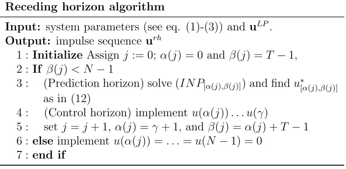
This section introduces a method to improve the bounds provided in the preceding section. The method is based on the receding horizon algorithm illustrated in Table 1. In the following, we first introduce the algorithm and then discuss its properties.
4.2.1. The algorithm
The algorithm receives uLP as input, and gives as output the impulse
sequence urh whose cost is J
rh := curh. We recall that uLP is an optimal
solution of (LP) in (10). The method consists in solving problem (IN P) online over a receding horizon [α(j), β(j)] with 0≤α(j)< β(j)< N. Let us denote by IN P[α(j),β(j)]
the problem solved at the generic iteration j. In addition, let us denote by u∗
[α(j),β(j)] the optimal solution of IN P[α(j),β(j)]
Receding horizon algorithm
Input: system parameters (see eq. (1)-(3)) and uLP.
Output: impulse sequence urh
1 : InitializeAssign j := 0; α(j) = 0 and β(j) =T −1, 2 : If β(j)< N−1
3 : (Prediction horizon) solve (IN P[α(j),β(j)]) and findu∗[α(j),β(j)] as in (12)
4 : (Control horizon) implement u(α(j)). . . u(γ)
5 : set j =j + 1, α(j) = γ+ 1, and β(j) = α(j) +T −1 6 : elseimplement u(α(j)) =. . .=u(N −1) = 0
[image:13.612.130.483.144.317.2]7 : end if
Table 1: Receding horizon algorithm.
We will show that u∗
[α(j),β(j)] has only one non-null component at time γ ∈ [α(j), β(j)], namely u∗
[α(j),β(j)] = (u
∗
(α(j)). . . u∗
(β(j)))′
where
u∗
(α(j)) = . . .=u∗
(γ(j)−1) = 0, u∗
(γ) = 1, u∗
(γ+ 1) =. . .=u∗
(β(j)) = 0. (12)
The problem solved at iterationj can be defined inductively. To do this, let us introduce the column vector of decisions over the horizon [α(j), β(j)]
u[α(j),β(j)] = (u(α(j)), . . . , u(β(j)))′,
and the feasible set
F[α(j),β(j)] ={u[α(j),β(j)] ∈ {0,1}T :
β(j)
X
k=α(j)
u(k)≥1}.
Now, let the receding horizon solution returned at iteration j−1 be
uj−1 := (u∗′
[0,α(j)−1], uLP ′ [α(j),N−1])
′
.
We recall that uLP
α(j) components. For j = 0, we initialize α(j) = 0, u∗
[0,α(j)−1] = nil and uj−1
:= uLP
[0,N−1]. Given the inductive reasoning, the solution u
∗
[0,α(j)−1] at
j − 1 is unambiguously determined once we clarify how to obtain uj =
(u∗′
[0,α(j+1)−1], uLP ′
[α(j+1),N−1])
′
, and in particular u∗
[0,α(j+1)−1] at iteration j. The problem solved at the generic iterationj is given by:
IN P[α(j),β(j)]
min
u[α(j),β(j)]∈F[α(j),β(j)]
cu (13)
u[β(j)+1,N−1] =uLP[β(j)+1,N−1]
u[0,α(j)−1]=u
∗
[0,α(j)−1]
x(k+ 1) =x(k) +f(x(k), d(k))
+ [h(x(k), d(k))−x(k)]u(k), k = 0, . . . , N −1.
Essentially, the vectors u[0,α(j)−1] and u[β(j)+1,N−1] are fixed and the opti-mization involves only the components in the interval [α(j), β(j)], namely
u[α(j),β(j)].
The interval extremes α(j) and β(j) are set as explained next. We set
α(j) equal to the first instant after an impulse has been activated, i.e.,
u∗
[0,α(j)−1](α(j)−1) = 1. We set β(j) so that
C1 the interval [α(j), β(j)] contains at most T candidate impulses, and
C2 the vector uLP
[α(j),β(j)] has only one non-null component, i.e.,
uLP(α(j)) = . . .=uLP(δ(j)−1) = 0, uLP(δ) = 1, uLP(δ+ 1) =. . .=uLP(β(j)) = 0.
In the above, we denote by δ the index (time instant) of the non-null component of uLP
[α(j),β(j)].
In other words, we set β(j) := min{α(j) + T − 1, r}, where r is the istant of a second impulse that should appear in uLP
[α(j),α(j)+T−1], formally,
r :={minrˆ∈[α(j),N−1]|
Prˆ
k=α(j)uLP[α(j),N−1](k) = 2}. To compute the solution uj = (u∗′
[0,α(j+1)−1], u
LP′
[α(j+1),N−1]) ′
, we need to compute the vectoru∗
[0,α(j+1)−1]. This is obtained by juxtaposition as clarified next. Let us consider two consecutive intervals [0, α(j)−1] and [α(j), α(j+ 1)−1]. Let the optimal solutions in the two intervals be
u∗
[0,α(j)−1] = (u ∗
(0), . . . , u∗
(α(j)−1))′
, u∗
[α(j),α(j+1)−1] = (u
∗
(α(j)), . . . , u∗
(α(j+ 1)−1))′
and juxtapose both solutions in order to define a new vector
u∗
[0,α(j+1)−1] = (u ∗′
[0,α(j)−1], u ∗′
[α(j),α(j+1)−1]) ′
. (14)
The solution returned by the algorithm at iteration j is then
uj = (u∗′
[0,α(j+1)−1], u
LP′
[α(j+1),N−1])
′
. (15)
Given u∗
[α(j),β(j)], we set α(j+ 1) =γ+ 1 and reiterate the procedure.
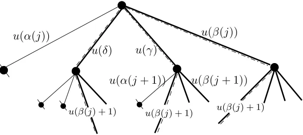
The method can be visualized using the decision tree displayed in Fig. 1.
u(α(j)) u(β(j))
u(δ) u(γ)
u(α(j+ 1)) u(β(j+ 1))
[image:15.612.153.461.274.411.2]u(β(j) + 1) u(β(j) + 1) u(β(j) + 1)
Figure 1: Decision tree illustrating the exploration of the solution domain.
There, edges correspond to variables and nodes correspond to time in-stants. The edges departing from any node identify the variables at future times. In particular, the edges at level 1 represent the decision variables
u(α(j)), . . . , u(β(j)) involved in IN P[α(j),β(j)]
. The dashed edge at level 1 corresponds to the non-null component uLP(δ) = 1 introduced in
condi-tion C2. The dashed edges at level 2 are all associated with the component of vector u[β(j)+1,N−1] which is fixed to one. We recall that in the definition of IN P[α(j),β(j)]
the vectoru[β(j)+1,N−1] is fixed. The algorithm builds upon the idea that u∗
[α(j),β(j)] has only one non-null component at time γ, as ex-pressed by (12). In addition to this, we have γ ≥ δ, where δ is the non-null component of uLP in [α(j), β(j)], as discussed in conditionC2. This is
4.2.2. Properties of the algorithm
Let us start by noting that problem IN P[α(j),β(j)]
guarantees the reverse dwell time condition on the interval [α(j), β(j)] from the definition itself of F[α(j),β(j)].
With regards to the setting of β(j), condition C1 is fundamental to guarantee feasibility of the solution returned by the algorithm as shown in Lemma 2, and furthermore it allows us to specialize the reverse dwell time conditions to [α(j), β(j)] and so we write them asu[α(j),β(j)] ∈ F[α(j),β(j)]. Con-ditionC2is critical to arrive at a solution not worse than uLP as established
in Lemma 3.
The next theorem establishes that u∗
[α(j),β(j)] has only one non-null com-ponent at time γ ≥δ, where δ identifies the non-null componentuLP(δ) = 1
as in condition C2.
Theorem 2. Solution u∗
[α(j),β(j)] has the structure given in (12), namely, for a generic integer γ ∈[α(j), β(j)] with γ ≥δ:
u∗
(α(j)) =. . .=u∗
(γ(j)−1) = 0, u∗
(γ) = 1, u∗
(γ+ 1) =. . .=u∗
(β(j)) = 0.
Proof. Given in the appendix.
The significance of the above result is mainly in that we can ignore earlier impulses (see the thin edges and pruned nodes in the decision tree of Fig. 1) thus reducing the computational complexity of the receding horizon algo-rithm. In this sense, an exhaustive search would imply to explore all thick edges. The provided algorithm reduces furtherly the computational burden as it fixes future decisions and this results in comparing uLP with only two
other solutions, emphasized in dash-dot in Fig. 1.
The next result establishes that the solution returned by the algorithm at iteration j, which is given in (15), satisfies the constraints of (IN P).
Lemma 2. The solution uj is feasible for the(IN P).
Proof. Given in the appendix.
Furthermore, it can be shown that the algorithm at each iteration re-turns a solution which is not worse than the one returned at the previous iteration. In other words, we have that uj improves uj−1
Lemma 3. For all j, it holds ∆J(j)≤0.
Proof. Given in the appendix.
The receding horizon algorithm returns a feasible solution in linear time as remarked next.
Theorem 3. The receding horizon solution urh is feasible for (IN P) and
provides a tighter upper bound:
JLP ≥Jrh ≥JIN P.
Also, the receding horizon algorithm finds urh in the worst-case in O(N).
Furthermore, if T = N then the solution urh is also optimal and the bound
is tight, i.e., Jrh =JIN P.
Proof. Given in the appendix.
The above result is a novelty as it uses geometric considerations borrowed from combinatorial optimization in a receding horizon context (see [20], part III.1 on integral polyhedra, p. 540).
5. Numerical Illustrations
This section provides a detailed numerical analysis of a simple network controlled system extracted from the queueing literature. The example adds another level of complexity in the optimization problem, namely, that of trying to stabilize simultaneously ten different systems instead of one. This reflects in the use of an additional scheduling component that concerns the selection of the system component (in this case a queue) that will receive the next impulse. Despite this new element, we can still reframe the example within the framework of ISS and reverse dwell time impulse control.
Assume we have queues describing demands accumulating at different geographic sites in a production/distribution inventory system. The system manager can serve only one queue (or site) at the time and up to a limited number of demands established by certain capacity constraints. Then, the queue lengths are the system state. Each time a queue is served an impulse acts on the corresponding system reducing the state of a fixed quantity. Each queue is described by the following impulsive dynamics. When no impulse occurs, for all i= 1, . . . , n,
˙
λ ρ x0 a ǫ N ˜c 50 150 rand([5,. . . ,10]) rand([0.8,. . . ,1]) 5(n32
[image:18.612.112.522.125.159.2]22 ) 1700 rand([1,. . . ,N]])
Table 2: Parameters of the experiment.
with rateai(t)>0 and whererand(−1,1) is a random disturbance uniformly
distributed in the interval between −1 and 1, ρ is the maximal disturbance. Furthermore, we assume that the impulse acts on the longest (in magnitude) queue. Then, denoting by ik = arg maxi|xi(tk)| such a queue, the impulsive
dynamics at impulse times is
xi(t+) =
xi(t)−sign(xi(t)) if |xi(t)|>1
0 if |xi(t)| ≤1
if i=ik
xi(t) if i6=ik
t=tk, k= 0,1,2, . . .
Note that the queues tend to diverge if no impulses are activated. So, roughly speaking, impulses have a stabilizing effect while the dynamics is unstable.
Serving a queue has a cost which depends on time, and also decreases with the queue length. In general, such a decreasing term models economies of scale [6]. This is a term used to describe situations where the cost of producing an additional unit of an outcome, (i.e, a good or service) decreases with the total volume of the outcome.
In mathematical terms, this means that activating an impulse has a cost
c(x(t), t) = K(t) + Ψ(V(x(t))) where the state dependent term is a linear decreasing function on the infinity norm of x(t), i.e., V(x(t)) =kx(t)k∞. In formulas, this corresponds to
Ψ(V(x(t))) =λ·max
t K(t)·
U B(kxk∞)− kx(t)k∞
U B(kxk∞)
,
where λ ≥0 and it is specified a-priori. We have denoted by U B(kxk∞) an
upper bound of the infinity norm of the state and we take for it the value 10. Parameter λ weights the influence of the state dependent term Ψ(V(x(t))) with respect to the time-varying term K(t). Actually, for kx(t)k∞ = 0, the term Ψ(V(x(t))) is λ times greater than the maximal time varying cost, maxtK(t).
Queues start from random values between 5 and 10, and the rate coefficients are randomly distributed from 0.8 to 1, i.e., ai = rand([0.8, . . . ,1]) for all
i = 1, . . . , n. The horizon length is N = 1700, and the values of K(t), or, which is the same, of the approximate costs ˜c are extracted randomly from the interval 1 to N.
Also, we take as time unit the value −log((ǫ−1)/ǫ) where ǫ = 10(n2322). This value is an estimate of the rate q used in (5) and it derives from the fact that between two consecutive impulses we can guarantee the condition kx(t+)k
2 ≤ ǫ−ǫ1kx(t)k2 at least on the average because of the random distur-bance rand(−1,1) (the same condition is always guaranteed in absence of a random disturbance). Beyond this, as the ratesaiare upper bounded by 1, we
can estimate the ratepused in (4) equal to 1, so that the value−log((ǫ−1)/ǫ) can also be taken as dwell time T for our simulations. The sample interval is 101 of the dwell time T =−log((ǫ−1)/ǫ), i.e., ∆t=−log((ǫ−1)/ǫ)0.1.
We simulate the receding horizon procedure starting at x(0). In the experiment, we compare the solutions of (9) and (8). The first solution is obtained by solving the linear problem
min
u∈P
˜
cu, P ={u∈RN : linear constraints (7),0≤u≤1},
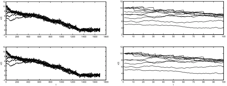
and returns a suboptimal cost. The second solution is the optimal solution obtained from the receding horizon algorithm. In particular, we illustrate the ISS properties of both solutions for a system with n = 10 independent queues.
In Fig. 2, left, starting from x0 = [8 10 8 10 10 7 5 6 10 10]′, the state is driven to the interval -1 and 1 at about t = 1200 and kept within such interval for the rest of the time. The two state trajectories are obtained by implementing the suboptimal control (top) and the optimal control (bottom). In Fig. 2, right, a zoom in the first 100 samples evidences the impulses and shows the difference between the two controls. The optimal control postpones the first impulse at about t = 10 (see, bottom) while with the suboptimal control the first impulse is att = 0 and thus, because of the effect of this first impulse, one of the five systems with initial state 10 actually evolves from 9.
6. Conclusions and future directions
0 200 400 600 800 1000 1200 1400 1600 1800 −2
0 2 4 6 8 10 12
x(t)
0 200 400 600 800 1000 1200 1400 1600 1800
−2 0 2 4 6 8 10 12
t
x(t)
0 10 20 30 40 50 60 70 80 90 100 2
4 6 8 10 12
0 10 20 30 40 50 60 70 80 90 100 2
4 6 8 10 12
t
[image:20.612.125.487.127.265.2]x(t)
Figure 2: Second experiment: time plot ofx(t) with approximate and exact controls (left).
Zoom on the first 10 samples (right).
From a theoretical perspective the obtained results have proved certain geo-metrical properties of the discrete set of feasible solutions. From a practical standpoint, such properties have reduced the computational burden thus making the algorithm suitable for the on-line implementation.
Appendix
Proof of Theorem 1
We start by observing that the constraint matrixA ∈ {0,1}m×N used in
the inequalities (7) turns out to be an interval matrix, i.e., it has 0-1 entries and each row is of the form
(0, . . . ,0 1, . . . ,1
| {z } 0, . . . ,0).
consecutive 1’s
Now, it is well known from the literature [20] that each interval matrix is totally unimodular where we remind here that a matrix istotally unimodular
if the determinant of any square sub-matrix is equal to−1, 0 or 1. This means that the polyhedron P is an integral polyhedron. As a consequence we have that the linear relaxation of the (ILP) has an integral optimal solution as established in the next lemma.
Lemma 4 ([2]). Solving (ILP) is equivalent to solving the linear program-ming problem:
(LP) min
u∈P
˜ cu.
Invoking the above lemma, we then have that uLP is also optimal for
(ILP). This means that (ILP) has at least one optimal solution uILP =
uLP. Then, we can substitute the latter solution in (IN P) thus obtaining
JLP =JILP and the first equality of (11) is proved.
To prove JILP ≥ JIN P observe that uLP belongs to F and as such it
is feasible for (IN P). In other words, we have uLP ∈ F which implies
JIN P = minu∈Fcu≤cu
LP and this concludes our proof.
Proof of Theorem 2
The underlying idea is to make use ofuLP
[α(j),β(j)] to find u
∗
[α(j),β(j)]. Let us introduce the subset of solutions with multiple impulses
I ={u[α(j),β(j)] :
β(j)
X
k=α(j)
Also, let us recall that uLP(δ) is the non-null component of uLP
[α(j),β(j)] and construct the subsetD ⊂ {0,1}T of solutions presenting one or more impulses
at any time earlier than δ, namely:
D ={u[α(j),β(j)] :
δ−1
X
k=α(j)
u(k)≥1, u(δ) =. . .=u(β(j)) = 0}.
Now, to prove (12) we need to show that u∗
[α(j),β(j)] is not in I nor in D as established next. Formally, solution u∗
[α(j),β(j)] 6∈ I ∪ D. To see that u∗
[α(j),β(j)] has a single non-null component, u
∗
[α(j),β(j)] 6∈ I observe that any other solution with additional non-null components would provide a higher cost.
To prove u∗
[α(j),β(j)] 6∈ D, it suffices to show that u
∗
[α(j),β(j)] dominates any other solution in D. To see this, we need to refer to Assumptions 2 and 1. Actually, it holds c(x(k), k) = K(k) + Ψ(V(x(k))) > ˜c(k) = K(k) for all k. Now, if the indexδgives the minimum to the cost with ˜c(k), then it gives also the minimum to the cost with c(x(k), k), because the sequence Ψ(V(x(k))) is decreasing on V(x(k)).
Proof of Lemma 2
We need to prove that uj ∈ F. The latter is true if
i) u∗′
[0,α(j+1)−1] satisfies conditions
Pβ(ˆj)
k=α(ˆj)u(k) ≥ 1 for all integer ˆj such that 0≤ˆj ≤α(j)−1, and
ii) uLP′
[α(j+1),N−1] satisfies
Pβ(ˆj)
k=α(ˆj)u(k)≥1 for all integer ˆj such thatα(j+ 1)≤ˆj ≤N −1.
Now, condition ii) is satisfied as uLP is feasible for (IN P). To prove
condition i) we first observe that solutionu∗
[0,α(j)−1] satisfies
Pβ(ˆj)
k=α(ˆj)u(k)≥1
for all integer ˆj such that 0 ≤ ˆj ≤ α(j)−1. We also note that u∗
Proof of Lemma 3
Note thatuLP
[α(j),β(j)] is feasible for IN P[α(j),β(j)]
asuLP
[α(j),β(j)] ∈ F[α(j),β(j)]. Invoking the optimality ofu∗
[α(j),β(j)](k) the we can infer the following inequal-ity which proves our thesis:
∆J(j) =
β(j)
X
k=α(j)
c(x(k), k)u∗
[α(j),β(j)](k) +
N−1
X
k=β(j)+1
c(x(k), k)uLP
[α(j),β(j)](k)
−
β(j)
X
k=α(j)
c(x(k), k)uLP
[α(j),β(j)](k) +
N−1
X
k=β(j)+1
c(x(k), k)uLP
[α(j),β(j)](k)
≤0.
Proof of Theorem 3
Let us show that JLP ≥ Jrh. Recalling that urh = uj
∗
where j∗
is the last iteration then we have Jrh−JLP =
Pj∗
j=0∆(j)≤0 the latter inequality being a consequence of Lemma 3. Then we have the thesis.
To prove that Jrh ≥ JIN P, note that urh is feasible for (IN P) from
Lemma 2. In other words, this means that urh ∈ F which implies J
IN P =
minu∈Fcu≤cu
rh and this concludes our proof.
To see that the receding horizon algorithm findsurh in the worst-case in
O(N) observe that the worst-case is when we have T equal to N. In the latter case it turns α(j) = 0, β(j) = N −1. If δ = 1 then the algorithm performs N comparisons between the solutions of S.
We next prove that if T = N then urh is optimal and J
rh = JIN P.
Actually, by definition we have urh :=u∗
[0,N−1]. Also observe that in this case
β(0) =N−1 and therefore u∗
[0,N−1] is optimal for (IN P[0,N−1]). Invoking the equivalence between (IN P[0,N−1]) and (IN P) we can conclude that urh is optimal for (IN P). As a consequence we haveJrh =JIN P and this concludes
the proof.
References
[1] D. Axehill, L. Vandenberghe, and A. Hansson, “Convex relaxations for mixed integer predictive control”, Automatica, vol. 46, 2010, pp. 1540– 1545.
[3] D. Bauso, “Optimal Impulse Control Problems and Linear Programing”,
Proc. of 48th IEEE Conference on Decision and Control Shangai, China, Dec. 2009, pp. 5299–5304.
[4] D. Bauso, Q. Zhu, and T. Ba¸sar. “Mixed Integer Optimal Compensa-tion: Decompositions and Mean-Field Approximations”, Proc. of the American Control Conference, 2012, pp. 2663-2668.
[5] F. Borrelli, M. Baoti´c, A. Bemporad, and M. Morari, “Dynamic pro-gramming for constrained optimal control of discrete-time linear hybrid systems”, Automatica, vol. 41, no. 10, 2005, pp. 1709–1721.
[6] D. D. Botvich and N. G. Duffield, “Large deviations, economies of scale, and the shape of the loss curve in large multiplexers”,Queueing Systems, vol. 20, 1995, pp. 293–320.
[7] M. S. Branicky, V. S. Borkar, and S. K. Mitter, “A Unified Framework for Hybrid Control: Model and Optimal Control Theory”, IEEE Trans. on Automatic Control, vol. 43, no. 1, 1998, pp. 31–45.
[8] C. G. Cassandras, D. L. Pepyne, and Y. Wardi, “Optimal control of a class of hybrid systems”, IEEE Trans. Automatic Control, vol. 46, no. 3, 2001, pp. 398–415.
[9] O. L. V. Costa, “Impulse control of piecewise-deterministic processes via linear programming”, IEEE Trans. on Automatic Control, vol. 36, no. 3, 1991, pp. 371–375.
[10] M.C.F. Donkers, P. Tabuada, and W.P.M.H. Heemels, “Minimum At-tention Control for Linear Systems: A Linear Programming Approach”,
Discrete Event Dynamic Systems Theory and Applications, vol. 24, no. 2, June 2014, pp. 199–218.
[11] M. Gazarik and Y. Wardi, “Optimal release times in a single server: An optimal control perspective”, IEEE Trans. on Automatic Control, vol. 43, no. 7, 1998, pp. 998–1002.
[13] Y. Guo, Y. Wang, L. Xie, and J. Zheng, “Stability analysis and design of reset systems: Theory and an application”, Automatica, vol. 45, no. 2, 2009, pp. 492–497.
[14] W. M. Haddad, V. Chellaboina, and S. G. Nersesov, Impulsive and hybrid dynamical systems, Princeton Series in Applied Mathematics, Princeton University Press, 2006.
[15] J. Hespanha, D. Liberzon, and A. Teel, “Lyapunov Characterizations of Input-to-State Stability for Impulsive Systems”, Automatica, vol. 44, no. 11, 2008, pp. 2735–2744.
[16] L. Hetel, J. Daafouz, S. Tarbouriech, and C. Prieur, “Stabilization of lin-ear impulsive systems through a nlin-early-periodic reset”,Nonlinear Anal-ysis: Hybrid Systems, vol. 7, no. 1, 2013, pp. 4-15.
[17] M. Jeanblanc-Piqu´e, “Impulse control method and exchange rate”,
Math. Finance, vol. 3, 1993, pp. 161–177.
[18] J. W. Lee and G. E. Dullerud, “Joint synthesis of switching and feedback for linear systems in discrete time”, Proc. of the 14th international con-ference on Hybrid systems: computation and control, 2011, pp. 201–210 ACM.
[19] F. Martinelli, C. Shu, and J. Perkins, “On the optimality of myopic pro-duction controls for single-server, continuous flow manufacturing sys-tems”, IEEE Trans. on Automatic Control, vol. 46, no. 8, 2001, pp. 1269–1273.
[20] G. L. Nemhauser and L. A. Wolsey, Integer and Combinatorial Opti-mization, John Wiley & Sons Ltd, New York, 1988.
[21] S. Monaco and D. Normand-Cyrot, “Advanced Tools for Nonlinear Sampled-Data Systems”, European Journal of Control, 13-23, Herm`es Sciences, Paris, 2007, pp. 221-241.