A Search for Extreme‐Ultraviolet Emission from Comets with the Cosmic Hot Interstellar Plasma Spectrometer (CHIPS)

A Search for Extreme#Ultraviolet

Emission from Comets with the Cosmic Hot

Interstellar Plasma Spectrometer (CHIPS)

The Harvard community has made this

article openly available.

Please share

how

this access benefits you. Your story matters

Citation

Sasseen, T. P., M. Hurwitz, C. M. Lisse, V. Kharchenko, D. Christian,

S. J. Wolk, M. M. Sirk, and A. Dalgarno. 2006. “A Search for

Extreme#Ultraviolet Emission from Comets with the Cosmic Hot

Interstellar Plasma Spectrometer (CHIPS).” The Astrophysical

Journal 650 (1): 461–69. https://doi.org/10.1086/507086.

Citable link

http://nrs.harvard.edu/urn-3:HUL.InstRepos:41397499

Terms of Use

This article was downloaded from Harvard University’s DASH

repository, and is made available under the terms and conditions

applicable to Other Posted Material, as set forth at

http://

A SEARCH FOR EXTREME-ULTRAVIOLET EMISSION FROM COMETS WITH THE COSMIC

HOT INTERSTELLAR PLASMA SPECTROMETER (CHIPS)

T. P. Sasseen

Department of Physics, University of California, Santa Barbara, CA 93106; tims@physics.ucsb.edu

M. Hurwitz

Space Sciences Laboratory, University of California, Berkeley, CA 94720

C. M. Lisse

Applied Physics Laboratory, The Johns Hopkins University, Laurel, MD 20723

V. Kharchenko

Harvard-Smithsonian Center for Astrophysics, Cambridge, MA 02138

D. Christian

Department of Pure and Applied Physics, Queens University, Belfast, UK

S. J. Wolk

Harvard-Smithsonian Center for Astrophysics, Cambridge, MA 02138

M. M. Sirk

Space Sciences Laboratory, University of California, Berkeley, CA 94720

and

A. Dalgarno

Harvard-Smithsonian Center for Astrophysics, Cambridge, MA 02138

Received 2006 January 22; accepted 2006 June 19

ABSTRACT

We have obtained EUV spectra between 90 and 2558of the comets C/2002 T7 ( LINEAR), C/2001 Q4 ( NEAT), and C/2004 Q2 ( Machholz) near their perihelion passages in 2004 with the Cosmic Hot Interstellar Plasma Spec-trometer (CHIPS). We obtained contemporaneous data on NEAT with theChandraACIS instrument, marking the first simultaneous EUVand X-ray spectral observations of a comet. The total CHIPS/ EUVobserving times were 337 ks for NEAT, 234 ks for LINEAR, and 483 ks for Machholz, and for both CHIPS andChandrawe calculate we have captured all the comet flux in the instrument field of view. We set upper limits on solar wind charge-exchange emission lines of O, C, N, Ne, and Fe occurring in the spectral bandpass of CHIPS. The spectrum of NEAT obtained with

Chandracan be reproduced by modeling emission lines of C, N, O, Mg, Fe, Si, S, and Ne solar wind ions. The measured X-ray emission-line intensities are consistent with our predictions from a solar wind charge-exchange model. The model predictions for the EUV emission-line intensities are determined from the intensity ratios of the cascading X-ray and EUV photons arising in the charge-exchange processes. They are compatible with the measured limits on the intensities of the EUV lines. For NEAT, we measured a total X-ray flux of 3:7;1012 _{ergs cm}2_s1_{and derive from model}

predictions a total EUV flux of 1:5;1012ergs cm2s1_{. The CHIPS observations occurred predominantly while the}

satellite was on the dayside of Earth. For much of the observing time, CHIPS performed observations at smaller solar angles than it was designed for, and EUV emission from the Sun scattered into the instrument limited the sensitivity of the EUV measurements.

Subject headinggs:comets: general — comets: individual (C/2002 T7 (LINEAR), C/2001 Q4 (NEAT),

C/2004 Q2 (Machholz)) — ultraviolet: solar system

Online material:color figures 1. INTRODUCTION

Soft X-ray emission has been detected from at least 20 comets since 1996. After the consideration and rejection of several pos-sible emission mechanisms, a consensus has been reached that the primary mechanism is charge-exchange collisions between highly charged solar wind minor ions and neutral atoms and mol-ecules of the cometary atmospheres, as suggested by Cravens (1997). The observations have been reviewed by Cravens (2002), Krasnopolsky et al. (2004), and Lisse et al. (2004). The solar wind charge-exchange (SWCX ) process also occurs in the heliosphere, where it contributes to the soft X-ray background (Cox 1988; Cravens 2000; Robertson & Cravens 2003; Pepino et al. 2004; Lallement 2004) and may be responsible for some fraction of the

short and- long-term enhancements seen at 250 eV (Snowden et al. 1995, 2004). These recent, interesting observations indi-cate that it is important to understand both the microphysics of the charge-exchange process and the phenomenology of where, when, and how this process occurs within the solar system.

Theoretical models of the X-ray and EUV emission lines pro-duced in comets by charge exchange with the solar wind ions have been constructed by Wegmann et al. (1998), Schwadron & Cravens (2000), Kharchenko & Dalgarno (2000, 2001), Kharchenko et al. (2003), Beiersdorfer et al. (2003), and Lisse et al. (2004).

Observations of diffuse SWCX emission other than from com-ets have been carried out usingChandra( Wargelin et al. 2004)

andXMM-Newton(Snowden et al. 2004). Wargelin et al. (2004)

observe the optically dark side of the Moon and attribute the 461

X-rays they detect to charge-exchange collisions between solar wind ions and neutral hydrogen in the Earth’s geocorona. Snowden et al. (2004) ascribe the emission they see as coming from the Earth’s exosphere or the heliosphere. In both cases, the emission is characterized by strong variability and correlation with the so-lar wind particle flux. X-rays generated by SWCX have been de-tected from the atmospheres of Mars and Venus ( Murawski & Steinolfson 1996; Dennerl 2002; Holmstrom & Kallio 2004; Fok et al. 2004; Gunell et al. 2004).

In summary, the highly ionized, heavy ions that stream out in the solar wind are a potential source of soft X-ray and EUV emis-sion from within the solar system. Charge-exchange emisemis-sion may occur, involving neutral atoms and molecules from comets entering the inner solar system, planetary exospheres, and neu-tral atoms in the interplanetary medium. A highly ionized solar wind ion may give rise to several photons, as the ion captures elec-trons sequentially in its flight from the Sun. A detailed ioniza-tion and density map of the heavy solar wind ions as a funcioniza-tion of time and position is required for a complete description of the X-ray and EUV emissions in the solar system. Measurements of SWCX emission from comets (and other measurements) can pro-vide a useful probe of the density and ion composition of the solar wind.

Many SWCX lines are predicted to appear at EUV energies below the low-energy limit of Chandra and XMM-Newton

( Kharchenko & Dalgarno 2000, 2001; Kharchenko et al. 2003). Some of these EUV lines arise from ions not conclusively iden-tified from emission at higher energies. These lines may be de-tected with CHIPS, a spectrometer sensitive in the EUV with a resolution of several hundred. The lines appear to be present in theRo¨ntgensatellit(ROSAT) PSPC spectrum of C/1990 K1 ( Levy) ( Dennerl et al. 1997), which rises steeply at energies be-low 200 eV. Krasnopolsky & Mumma (2001) observed comet C/1996 B2 ( Hyakutake) at low resolution at EUV wavelengths and claimed detection of lines from O, C, He, and Ne. Kharchenko & Dalgarno (2001) predict that, at lower energies, emission lines from the Ovidoublet at 1032 and 10388should be the brightest

far-ultraviolet ( FUV ) SWCX lines. A sensitive search for EUV and FUV emission lines in cometary SWCX was conducted with theFar-Ultraviolet Spectroscopic Explorer(FUSE) observatory ( Weaver et al. 2002; Feldman 2005). Weaver et al. (2002) report a tentative detection of 10328emission lines from comet C/2000 WM1 (LINEAR). An alternative interpretation of this feature has been suggested by Feldman (2005) fromFUSEobservations of the brighter comet C/2001 Q4 ( NEAT); they attribute this feature to H2fluorescent emission lines pumped by radiation from Niii

and Oviions in the solar corona. The nondetection of the brightest

FUV Ovilines from SWCX may be because the relatively small

field of view ofFUSEallowed observation of only about 6000– 7000 km around the cometary nucleus. For the Q4FUSE observa-tions, the peak brightness of the charge-exchange EUV and X-ray emissions was shifted by more than this amount from the comet center, and hence theFUSEaperture may have missed it (Feldman 2005).

The favorable perigee passages of the bright comets C/2001 Q4 ( NEAT ) and C/2002 T7 ( LINEAR) in 2004 May and Machholz in 2005 January provided an excellent opportunity to use the unique low-energy spectroscopic capabilities of CHIPS to study SWCX in comets at EUV wavelengths. Due to a combi-nation of high solar activity and their close approaches, comets C/2001 Q4 ( NEAT) and C/2002 T7 ( LINEAR) are the brightest X-ray targets available since C/ Hyakutake in 1996 and 153P/2002 C1 ( Ikeya-Zhang) in 2002. In this paper, we discuss the observa-tional data from CHIPS andChandra, describe the procedures by

which we measure the line strengths, and discuss the implications for the cometary charge-exchange process.

2. OBSERVATIONS AND DATA REDUCTION 2.1.Instrumental

The CHIPS orbit is approximately circular at 600 km and an in-clination of 94, determined by the primary payload ( ICESAT) of the rocket that launched the instrument. CHIPS is sensitive to the EUV band of 90–2608, or 47–138 eV. With all six slits open, the spectrograph field of view is roughly rectangular at 5;25Any object smaller than a few degrees presents a ‘‘point’’ source to CHIPS and will be visible only through two slits at a time. The observations presented here were collected in wide-slit mode, with a peak resolution for diffuse light of ~3.48FWHM, reaching ~ 48at the edges of the bandpass.

Light from the comet enters the CHIPS spectrograph through two slits, each 1 mm;7 cm. The light diverges onto an 8;6 cm grazing-incidence cylindrical diffraction grating with a central groove density of 1800 lines mm1_{. The groove density is varied}

across the grating surface to provide nearly stigmatic focusing in the dispersion direction near the center of the spectral band. Thus, the spectral resolution near the center of the band is limited by the slit width. At the ends of the band, the combined effects of opti-cal aberration and defocusing contribute to the net spectral line width. For sources that are significantly smaller than the field of view of a slit, the resolution is independent of the angular size of the comet.

The grating rulings and baffling reject most non-EUV light, and thin-film filters placed close to the detector also attenuate out-of-band and scattered light. A diffuse emission line spans the full available detector height, typically passing through two dif-ferent filter materials: aluminum, zirconium, or polyimide / boron. Measurements of an emission line that has the appropriate ratio of line flux from the two different filters spanned by the line en-courage the belief that an actual spectral line has been detected and not some detector artifact.

The CHIPS in-orbit calibration is discussed in more detail in Hurwitz et al. (2005), and additional details of the science instru-ment and the CHIPSat satellite are presented in Hurwitz et al. (2003, 2005), Janicik et al. (2003), Marckwordt et al. (2003), Sirk et al. (2003), and Sholl et al. (2003).

2.2.Comet Obser

v

A summary of the CHIPS observations of all three comets is presented in Table 1. We co-add individual comet observa-tions in different subsets as described below. Individual point-ings are of20 minute duration and, owing to the orbital geometry, nearly all observations took place while the satellite was on the dayside of Earth. The CHIPS mission has a nominal constraint of 72for the minimum boresight-to-Sun angle permitted during observations, both for spacecraft health reasons and to minimize the amount of scattered solar radiation entering the spectrometer. However, observing NEAT Q4 and LINEAR T7 near their time of maximum optical brightness required observations that vio-lated this Sun-angle constraint and required the development and use of a new observing mode to accommodate the smaller solar angles, as well as observe a target moving in the sky. The two most important differences for this mode are a slightly reduced pointing accuracy and stability, since the main Sun sensor did not have the Sun in the field of view, and a possible increase in the amount of scattered solar EUV radiation present in the comet spectra.

Initial data reduction was carried out using the pipeline that is described in Hurwitz et al. (2005). We apply several filters to the SASSEEN ET AL.

raw data in producing the reduced spectra. Data are excluded when the overall detector count rate exceeds 80 events s1_,

indic-ative of high charged-particle backgrounds. Data are also excluded when the detector high voltage is reduced (a normal, temporary response to transient high-background periods). A broad pulse-height filter is applied by the flight software. Approximately 40% of the telemetered events are then excluded by a low-pass pulse-height threshold in ground software, selectively reducing back-ground because the low-amplitude events are overwhelmingly triggered by charged particles, rather than by photons.

Periodically pulsed ’’stimulation pins’’ outside the active field of view are used to register the event (X, Y) coordinates to a com-mon frame, thereby correcting for thermal drifts in the plate scale or axis zero points, and to determine the effective duration of the observation. Distortion is corrected using a preflight pinhole grid map. Small regions of known detector ‘‘hot spots’’ are excluded, the event coordinates are rotated so that the newX-axis closely corresponds to the spectral dispersion direction, and the spectra in each filter half are summed over the active detector height.

Once the final spectra (one each from the upper and lower detector halves) have been summed, these will typically contain counts from several background sources in addition to any signal from a comet. The primary backgrounds include particle events that are generally uniform across the detector, geocoronal Hei

5848photons that are scattered by the gratings and penetrate the Al filters, and for these comet observations, some EUV photons from the Sun that are multiply scattered from some structure on the satellite into the spectrometer. These backgrounds must be properly accounted for or subtracted before we can assess the amount of radiation from the comets that may be present.

We show in Figure 1 the summed spectra from all the indi-vidual NEAT Q4 observations, totaling 329,495 s of useful data. The upper curve is the polyboron/Al side of the detector, while the lower trace is the Zr/Al side of the detector, lowered by 200 counts. The wavelength ranges of the various filters are indicated, as are the positions of the filter-supporting bars for each half. The continuum seen in the poly/B and Zr filters is primarily from par-ticle events, while the Al filters show a significant additional smooth background from scattered geocoronal Hei5848

pho-tons. The effective area of the spectrometer as a function of wave-length is shown in Sirk et al. (2003). We add together signals from one or both halves of the detector at a particular wavelength based on the filter transmission curves to maximize signal-to-noise ratio (S/ N ) at that wavelength or to exclude artifacts. The ranges in-cluded from each filter/half are indicated in Figure 1.

To determine the continuum against which to search for emis-sion lines, we use a very deep flight charged-particle spectrum, scaled to match the local counts in the spectrum under analysis. The deep charged-particle spectrum generally contains many more

events per wavelength interval than does the spectrum under anal-ysis, and thus contributes relatively little to the shot noise in the line flux. Differences in the technique by which the scale factor is determined, for example, heavy smoothing versus fitting low-order polynomials, result in changes of10% to the line-flux re-sults. To determine the absolute ‘‘flatness’’ of the detector response, we analyzed a preflight photon flat field that was histogrammed like the flight spectra. Compared to a smooth polynomial, the flat-field spectrum showed a pixel-to-pixel variance only slightly greater than that expected for shot noise, where ‘‘pixel’’ refers to the width of the narrowest spectral features. The excess 1 var-iance above shot noise was ~0.3% of the total signal. This factor is negligible in all the limits reported here, where shot noise from charged particles detected is the dominant uncertainty.

We measure the line flux of an individual line by adding all the counts that occur within one spectral resolution element of the line-rest wavelength, and subtracting the counts summed from the scaled background spectrum over the same limits.

The wavelength scale is based on preflight measurements, offset by a (constant)1 8 determined from the bright geo-coronal Heii256.38feature, which is present in essentially all

the observations. Temporal variations in the measured centroid of the Heiifeature show a dispersion of ~0.28. Periodic

obser-vations of the moon, which provide a weakly reflected solar spec-trum that includes lines of Feix–Fexii, confirm that the adopted

wavelength scale provides a good fit near the center of the spectral band and support the view that the relative throughput of the filter panels is as measured preflight. The measured fluxes of both the Heiifeature and the lunar spectrum are in good agreement with

preflight expectations, suggesting that the instrument throughput has not declined since laboratory calibration. The preflight lab-oratory throughput calibration tied to an NIST-calibrated diode, both at a component level and an end-to-end manner (which agree to within10%), provides the absolute flux calibration.

2.3.PointingStability

The CHIPS at attitude control system (ACS) is described in Janicik et al. (2003). The ACS uses inputs from several sensors, including coarse and medium Sun sensors, magnetic sensors, a lunar sensor, and reaction wheel rotation sensors to calculate the spacecraft attitude. During most of the observations reported here, CHIPS was unable to use its most accurate source of atti-tude information, the spacecraft’s medium Sun sensor. Instead, the adopted observing procedure was to orient the spacecraft such that the Sun was in the Sun sensor for the fraction of each orbit when a comet was not being observed, then slew to the comet during the period when the comet was visible. When the Sun sensor is used, the typical pointing accuracy of the spacecraft is within0N5 of the requested target (Janicik et al. 2003) and

TABLE1

Summary of CHIPS Comet Observations

Comet (1) Date Range Observation (CHIPS) (2) Exposure Time Day (s) (3) Exposure Time Night (s) (4) Sun Angle Range (deg) (5) Sun-Comet Distance Range (AU ) (6) Earth-Comet Distance Range (AU ) (7) VMagnitude Range (8)

0.25–1 keV Flux (1012_ergs

cm2_s1₎ (9)

C/2001 Q4 ( NEAT )... 2004 Apr 21 07:35–2004 May 21 07:39 331096 5832 78.1–69.0 1.05–0.97 0.58–0.56 2.6–2.1 3.7 C/2002 T7 ( LINEAR) ... 2004 May 02 11:45–2004 May 31 03:41 219477 14415 40.0–72.8 0.65–1.0 0.76–0.55 1.5–2.7 . . .

C/2004 Q2 ( Machholz) ... 2005 Jan 06 23:44–2005 Jan 28 22:58 441466 41158 130.3–106.7 1.24–1.21 0.35–0.47 4.1–4.7 . . .

centered to within 1/10 of the spectrometer field of view. For rel-atively short periods, even with slews, such as a typical 25 minute comet observation, the spacecraft reaction wheels provide point-ing orientation and knowledge, with negligible degradation. This is confirmed by the very small attitude corrections that followed reaquisition of the Sun by the medium Sun sensor.

In the CHIPS observations of the comets, we conclude that es-sentially all of the EUV-emitting region of the comet is contained within the CHIPS entrance apertures during the observations. The field of view of the two central slits of CHIPS is approxi-mately 5 deg2. Comet positions were generated every 10 minutes during the period they were observed by CHIPS using the Minor Plant and Comet Ephemeris Service,1where the requested point-ing corresponded to the midpoint in time of each observation. Parallax and the motion of the comet during an orbit’s pointing are negligible compared with the CHIPS field of view. Our re-mapped image of Q4 on theChandraACIS-S detector shows the X-ray–emitting region to be no larger than 100;100. Given the attitude information and the size of the X-ray emitting region, we believe that the comets were positioned in the slit entrance ap-erture when the spacecraft reported that it was pointed at the re-quested comet position and that the emitting region was fully contained within the CHIPS field of view. Hence, for the obser-vations reported here, we assume no dilution factor for comet EUV emission. The roll angle for observations was chosen such that the CHIPS entrance slits were perpendicular to the great circle that contained both the comet and the Sun.

2.4.Background / Noise Sources

The majority of counts registered in the CHIPS detectors are from charged particles entering the instrument. Although some discrimination against particle events based on pulse height takes place as described above, the time-varying nature of this back-ground makes it difficult to determine the presence of any con-tinuum emission arising from photons. The net effect of the backgrounds and data-reduction techniques is that CHIPS is primarily sensitive to spectral lines, with a limiting sensitivity of a few line units or LU ( photons cm2s1sr1) for the obser-vations described here.

CHIPS consistently detects at high-significance Heiiemission

arising in the Earth’s geocorona at 256.38and, to a lesser de-gree, at 243.08. In addition, we observe radiation that appears to originate in the solar corona and is multiply scattered from sur-faces on the spacecraft into the instrument. Although this back-ground is very faint compared with the interstellar medium emission lines from Feix–Fexiithat CHIPS was designed to

observe, we have studied it in depth, because it is a significant background to these measurements. The EUV line emission from the interstellar medium reported by Hurwitz et al. (2005) based on 1 yr of CHIPS observations is very faint and does not pose a significant background for the comet observations. A de-tailed study of the instrument-scattered background shows that the lines are never seen in co-added nighttime- only observa-tions, and the spectrum appears very similar to the full-Moon spectrum. The strength of the lines does not correlate with the zenith angle, the lines show no ram-angle dependence, and they appear reproducibly in only a relatively small number of

1 _{See http://cfa-www.harvard.edu /iau / MPEph / MPEph.html.}

Fig.1.— Complete CHIPS spectrum after pipeline processing using all data from C/2001 Q4 ( NEAT ) on the two detector halves, shown in counts. The lower spectrum has been displaced by 200 counts for clarity. The filter bandpasses and edges, location of known solar and geocoronal lines, and detector/ light artifacts that show up in all CHIPS spectra are marked. Vertical marks show the location of charge-exchange lines predicted in this band from comets. Our flux detection limits for a particular line use one or both halves (indicated by lines at the top of the figure; Poly/ B/Al top, Zr /Al bottom) to optimize the S/ N at that wavelength.

SASSEEN ET AL.

spacecraft orientations relative to the Sun. The lines appear more often, but not always, when CHIPS points closer to the Sun than during normal observations, but there is not a significant anti-correlation with the solar-target angle. The line strengths show no correlation with the Ultra Low Energy Isotope Spectrometer ( ULEIS; Mason et al. 1998) measurements of Feix, Fex, and

Fexiin the solar wind during the time of the comet observations,

and the line strengths during comet observations do not correlate with measurements of solar disk irradiance in the 170–2308by the Solar EUV Experiment on TIMED (SEE; Woods et al. 1998). We conclude that the source of these background lines is faintly scattered radiation from the solar corona. Owing to its appearance preferentially at smaller solar angles, this background is therefore of more importance for the CHIPS comet observations than dur-ing normal sky survey observations, which are made at larger so-lar angles.

Figure 2 shows the co-added lunar spectrum observed by CHIPS in narrow-slit mode from several months in 2003 and the co-added spectrum from a number of observations, when the background lines were strongest. The similarity of the spectra is evident, although we would not expect identical spectra because the solar spectrum itself varies, and the scattered spectrum was taken in wide-slit mode, which is more sensitive to the scattered radiation and has lower spectral resolution. We can nonetheless use either the Moon spectrum or the co-added bright background times as a template to indicate the possible presence of solar-scattered lines in the following way. We developed this indicator by first subtracting the continuum level from the scattered light spectrum after fitting it with a polynomial. We then similarly fit and subtract the continuum from another CHIPS observation. When the two continuum-subtracted spectra are multiplied to-gether in the region of the lines, the template acts as a matched filter, sensitive to the solar lines. We call the exposure-time-normalized product of the two spectra integrated over the spec-tral region 170–2308the ‘‘line-flux indicator,’’ or LFI. We find

the LFI to be a sensitive indicator of the presence of scattered so-lar light in co-added observations and can use it to reject data that contains this background where required. The third trace in Fig-ure 2 is co-added daytime data selected for low LFI and shows essentially no solar contamination. However, in most cases we measure only upper limits to the spectral lines expected from charge-exchange reactions, so that the presence of a possible solar background is of less concern than it would be were CX lines detected. In addition, the CX lines we are trying to detect form an only partially overlapping set with the lines emerging from the so-lar corona.

We show in Figure 3 the relative LFI value for each day of the Q4 and T7 CHIPS observations. We also show the scaled mag-nitude of the solar 170–2308flux of the Sun as measured by SEE, which does not correlate with the LFI values. Finally, we also show a model of the visual brightness of the two comets, where the variation is based only on the inverse-squared distances from the Earth to the comet and the comet to the Sun. The latter curves indicate that we observed Q4 through its peak brightness, while the T7 observations were only possible as the brightness declined, since the comet was too close to the Sun in the sky to be observed prior to that time. Owing to the sensitivity level of the CHIPS data, it is not useful to subdivide the data into different time slices to investigate possible time variation of the emission.

2.5.Chandra Obser

v

Comet C/2001 Q4 ( NEAT) was observed by Chandra on 2004 May 12 using director’s discretionary time. The total ap-proved observation of 10 ks was divided into three pointings of approximately equal length. During each observation the tele-scope was held fixed, and the comet allowed to drift through the field of view. The comet was centered on the S3 chip, which has the best low-energy response. The three resultant standard level 2 event lists were simultaneously concatenated and reprojected

Fig.2.— CHIPS dayside comet and lunar spectra through Al ( polyimide/ boron detector half ) filter and standard pipeline processing. The spectra are not divided by the filter response. The upper trace shows a set of co-added CHIPS observations, selected when the dayside background lines are brightest. The mid-dle trace shows a set of dayside spectra, chosen with low LFI, showing no solar contamination. The lowest trace shows the co-added full-Moon spectrum, taken for calibration purposes by CHIPS in narrow slit mode. The lines visible in the lunar spectrum arise from the solar corona being reflected by the Moon. The similarity in the spectral lines points to an origin in the solar corona for the dayside lines in the nonlunar spectra as well.

into a fixed ‘‘comet-centered’’ frame of reference using the CIAO2 toolsso_freeze. The final reconstructed image provides good spatial (0B5 pixel1) and spectral information (50 eV).

A source spectrum was extracted from a circular aperture with a radius of 700 pixels (5A8) centered on the peak of the comet emission, and the background spectra were extracted from the area outside the source aperture. We examined how varying the aperture radius changed the comet and background spectrum. The aperture radius we chose included essentially all of the emis-sion from the comet; outside of this radius, we expect that helio-spheric SWCX will be a uniform background on this scale. The background spectrum normalized by area was subtracted from the in-aperture spectrum to produce the Q4 comet spectrum. Work by Lisse et al. (1996) and Wegmann & Dennerl. (2004) shows that the CX X-ray emission from a comet as active as Q4 may be offset from the nucleus by 30,000–40,000 km. At the dis-tance of 0.6 AU, where Q4 was observed withChandra, this sep-aration translates to an angle of10. Owing to the diffuse nature of the emission and the positional uncertainty induced by the photon remapping, it is not clear whether we can discern a potential offset of this magnitude from the center of the nucleus, but we have verified that the spectrum resulting from our chosen aperture radius is insensitive to a potential offset of this size. A detailed discussion of the Q4 X-ray emission morphology will be covered in C. M. Lisse et al. (2007, in preparation). ACIS re-sponse matrices for modeling the instrument-effective area and energy-dependent sensitivity were created with the standard CIAO tools, and the resulting spectra were fit using XSPEC.

3. RESULTS AND DISCUSSION

Figure 1 shows the C/2001 Q4 ( NEAT) spectrum from 50 to 2708measured with CHIPS. For each potentially strong charge-exchange spectral line indicated in the figure, we measure the brightness using the spectra from one or both halves of the CHIPS detector. We have run our line-flux measuring algorithm for each comet, and the results of these measurements are shown in Table 2.

We include two measurements using the Q4 data: (1) the ‘‘no-LFI’’ set, referring to the period 2004 May 9–19, corresponding to a time when the LFI measurement indicates minimal contamination from scattered solar EUV radiation and (2) the line limits when us-ing all the Q4 CHIPS data. We also present the limits from a spec-trum consisting of the co-added spectra from all three comets, which contains the lowest relative shot-noise background. We measure positive flux at the wavelengths of a number of poten-tial charge-exchange lines, albeit at low significance.

Fe lines at wavelengths 170–2208are detected in several of the spectra at significances ranging to 5. Since it is likely that much or all of this emission is solar rather than cometary, we re-strict our consideration to possible charge-exchange lines short-ward of 170 8, although line measurements that may have a solar component provide upper limits to the cometary emissions. We estimate that the lines for which we report limits in the table contribute about 90% of the flux from charge exchange, if we ignore the iron lines.

The least contaminated spectrum is that obtained from the NEAT Q4 data selected for low LFI, and the most significant line is the Oviline at 129.918, at almost 2, arising from the

1s4d3_D–1s2p3_Ptransition.

In Figure 4, we show the results, binned to the CHIPS instru-mental resolution, of the line-flux measuring algorithm run on a 18wavelength grid on the combined data set. When using this technique, a positive actual line flux suppresses the neighboring continuum. Hence, positive flux should be read from the graph axis, not the adjacent continuum. Tentative line identifications of features associated with positive flux measurements are indicated. The feature at 91.18coincides with the transition 1s4p3P–1s2s3S

of Ovii, and the feature at 128.58to the 1s3d3D–1s2p3P

tran-sition. Ovihas lines at 116.4, 129.9, 132.5, and 150.18,

corre-sponding respectively to the 4p–2s, 4d–2p, 4s–2p, and 3p–2s

transitions.

A search for line detections can also be conducted using theo-retical predictions for the wavelength and flux ratio of several lines from the same ion. We employed the nine brightest lines in the CHIPS band of the Oviion given by the model described in

2 _{ChandraInteractive Analysis of Observations.}

TABLE2

Charge-Exchange Line-Flux Limits

C/2001 Q4 No-LFI C/2001 Q4 C/2002 T7 C/2004 Q2 All Combined

Wavelength(8) Ion Limit Sign. Limit Sign. Limit Sign. Limit Sign. Limit Sign. 98.37... Neviii 0.22 _{1.63 0.00} 0.87 _{1.03 0.00} 2.58 _{1.23 0.00} 1.00 _{0.89 0.00} 1.30 _{0.63 0.00} 115.86... Ovi 0.51 _{0.77 0.00 0.26 0.48 0.53 1.01 0.58 1.74 0.19 0.42 0.45 0.39 0.30 1.31} 120.33... Ovii _{0.20 0.76 0.27 0.14 0.47 0.29} 0.83 _{0.56 0.00} 0.62 _{0.41 0.00} 0.42 _{0.29 0.00} 128.48... Ovii 0.26 1.07 0.25 0.06 0.66 0.09 0.10 0.78 0.12 0.64 0.56 1.13 0.33 0.40 0.84 129.91a_{... Ovi 2.22 1.16 1.92 0.52 0.71 0.73}

0.34 0.83 0.00 0.56 0.60 0.93 0.35 0.43 0.82

132.35a_{... Ovi 0.56 1.24 0.45 0.83 0.76 1.10 0.14 0.89 0.15}

0.29 0.64 0.00 0.17 0.46 0.36

133.92... Nvii 0.04 1.29 0.00 1.07 0.80 1.34 0.40 0.94 0.42 0.69 0.67 0.00 0.11 0.48 0.24 135.02... Cvi 0.27 1.31 0.00 0.27 0.81 0.34 0.34 0.95 0.36 0.08 0.68 0.00 0.12 0.48 0.26 150.21... Ovi 1.84 1.60 0.00 0.21 0.97 0.00 1.09 1.14 0.00 0.15 0.82 0.19 0.24 0.58 0.00 173.29... Ovi 1.84 2.02 0.91 5.16 1.26 4.10 3.48 1.57 2.22 1.85 0.87 2.13 3.27 0.73 4.49 182.28... Cvi 0.64 2.56 0.25 2.76 1.63 1.69 6.13 2.11 2.91 0.69 1.02 0.00 1.90 0.95 2.00 184.19... Ovi 2.95 2.56 0.00 1.96 1.63 0.00 7.77 2.10 0.00 0.55 1.03 0.54 2.06 0.95 0.00 186.74... Cv 2.15 2.60 0.83 0.47 1.65 0.00 0.47 2.14 0.00 1.59 1.04 1.53 0.48 0.97 0.50 197.05... Cv 0.11 2.80 0.04 6.09 1.80 3.37 11.65 2.36 4.93 0.50 1.12 0.45 4.72 1.05 4.48 209.44... Nv 2.15 3.20 0.67 2.88 2.03 0.00 3.61 2.61 0.00 1.81 1.27 1.43 0.87 1.18 0.00 227.20... Cv 4.84 3.14 1.54 3.42 1.96 1.75 5.15 2.43 2.12 1.01 1.23 0.00 1.75 1.13 1.55 248.75... Cv 8.32 4.38 1.90 2.06 2.74 0.75 7.36 3.40 2.16 6.14 1.76 0.00 0.57 1.60 0.00

Note.—Limit and localvalues in LU. Sign. = limit /. To find a limit in photons cm2s1, multiply the value in LU by 0.0106. a

Indicated lines and those withk>1708are subject to contamination from solar Feviii–Fexiiemission.

SASSEEN ET AL.

the following section. The line profiles were taken to be Gaussian, with widths equal to the wavelength-dependent resolution of CHIPS. The free parameters in the fit were a quintic polynomial used to find the background level and an overall amplitude for the Ovilines, with the individual line ratios fixed. The results when

this technique was applied to the NEAT Q4 no-LFI spectrum are that the line amplitudes are consistent with zero. We carried out the same procedure for the co-added comet T7 spectra, and again the results were consistent with zero Oviemission.

4. MODELING THE SOLAR WIND CHARGE-EXCHANGE EMISSION

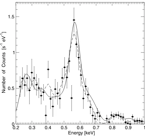
The NEAT Q4 count spectrum obtained fromChandrais shown in Figure 5. It contains emission lines seen in other comets ( Lisse et al. 2001; Krasnopolsky et al. 2002). We first use XSPEC to fit the spectrum with eight emission lines whose wavelengths were allowed to vary. The best fit was achieved with eight lines at en-ergies in eV of 245, 320, 403, 496, 570, 655, 830, and 952, with corresponding photon fluxes in units of 104_{photons cm}2_s1_of,

respectively, 3.68, 26.5, 6.57, 2.59, 5.93, 1.05, 0.29, and 0.11. The resulting2_{per degree of freedom was 0.91. The strong lines at}

320, 403, and 570 eV correspond to transitions of Cv, Nvi, and

Ovii. The lines near 245 eV may be from Siix, Mgix, or Mgx,

and a feature at 952 eV, found also in the spectra of comets McNaught-Hartley and LINEAR 4 ( Krasnopolsky et al. 2002, 2004), may be from Neix. There is an indication of a line near

835 eV, but we hesitate to attribute it to the 5p–1sresonance line of Oviii, because we do not find the corresponding 2p–1sline at

653 eV, which we predict should be more intense by a factor of 6. Because of the low resolution of the instrument, fits with a similar2figure of merit are also obtained by a combination of emission lines and thermal bremsstrahlung at a temperature of about 0.23 keV, as in Kharchenko & Dalgarno (2000).

We have extended a model developed by Kharchenko & Dalgarno (2000, 2001), Kharchenko et al. (2003), and Pepino et al. (2004) to compute emission spectra over the full EUV and X-ray spectral range. In the model, we use electron-capture cross sections for positive ions colliding with neutral H2O molecules

that reproduce the experimental laboratory X-ray spectra when available and theoretical estimates when they are not ( Rigazio et al. 2002). When applied to the measured spectra, the method takes into account empirically determined processes, such as mul-tiple capture followed by autoionization. The capture cross sec-tions determine the entry rates into the individual excited states of the ion created in the charge exchange. The excited states decay in a radiative cascade which produces photons at X-ray, EUV, and UV wavelengths. The relative intensities of the emission lines oc-curring in the cascade from a given initial level depend only on the branching ratios of the transition probabilities. Thus, the EUV spectrum is determined by the X-ray spectrum, and the comet spectra depend on and provide a measure of the solar wind ion composition.

4.1.X-Ray Emission Lines

We calculated the X-ray emission-line intensities for the ion composition listed in Table 3. It is based on the ion composition of Schwadron & Cravens (2000) for a fast solar wind, supple-mented by the presence of a fraction of 0.001% of highly charged Fe ions, Fexv–Fexx, that appear to be necessary to reproduce the

observed spectrum between 0.8 and 0.9 keV. An enhanced flux of highly charged iron ions may be a consequence of fast coronal mass ejection events ( Lepri & Zurbuchen 2004; Zurbuchen et al. 2004).

A comparison of the observations in counts per second of NEAT Q4 and the XSPEC and SWCX models at photon energies between 0.3 and 1.0 keV is presented in Figure 5. TheChandra

data with the error bars indicating 1uncertainties are shown as filled circles. The dashed line is the XSPEC model fit, with eight emission lines folded through the instrument response. The solid line is the SWCX prediction at a spectral resolution of 75 eV. In Table 4, we list the energies and wavelengths and the predicted

Fig.4.—All three comet spectra summed, then continuum subtracted. This procedure can improve the visibility of strong emission lines, but is subject to uncertainties in the continuum level placement. Spectra and errors shown at 48 resolution, close to the actual instrument resolution, and the error bars are 1. Some tentative spectral line identifications are indicated. Longward of 1708, solar Fe lines dominate the spectrum.

Fig.5.—Two models of X-ray emission lines are compared with theChandra spectrum for C/2001 Q4 ( NEAT ). The filled circles are the number counts from

relative intensities of the principal X-ray and EUVemission lines of the SWCX model. The agreement of the measurements of the X-ray lines with the models is good, but because of the low spectral resolution, we cannot exclude a significant contribution from bremsstrahlung from XSPEC modeling of the X-ray lines alone.

4.2.EUV Emission Lines

The photon fluxes measured for NEAT Q4 with CHIPS at energies below 150 eV and withChandraat energies between 250 eVand 1.0 keVare compared in Figure 6 with the predictions of the SWCX model. A scaling factor has been applied to bring the predicted total flux of the X-ray emission with energies greater than 250 eV into agreement with the measured value of 3:7; 1012ergs cm2s1. Table 4 can then be used to yield the absolute intensities shown in Figure 6. The corresponding total flux of the EUV lines between 47 and 140 eV is 1:5;1012_{ergs cm}2_s1_,

distributed among 181 lines of C, N, O, Ne, and Fe. The

theo-retical EUV intensities fall well below the measurements except near 95 eV, a region in which several lines of Oviand Oviiappear.

The most interesting CHIPS measurement of the SWCX lines is the 2detection in the NEAT Q4 no-LFI spectrum of the line of Oviat 95.5 eV, or 1308. Discrepancies at lower energies are

af-fected by scattered radiation from the Sun. We conclude that the SWCX model EUV predictions are consistent with the CHIPS data, but the instrument lacks the sensitivity needed to system-atically test the theoretical predictions. In that CHIPS was not

TABLE3 Solar Wind Ion Composition

Ionization State

Atom 5+ 6+ 7+ 8+ 9+ 10+ 11+ 12+ 13+ – 20+

C... 0.058 0.004 . . . .

N... 0.0074 0.0012 0.0009 . . . .

O... . . . 0.053 0.004 . . . .

Ne ... . . . 0.006 0.00006 . . . .

Mg ... . . . 0.0025 0.0017 . . . .

Si ... . . . 0.0015 0.0014 0.00007 . . . .

S ... . . . 0.0004 . . . .

Fe... . . . 0.0015 0.015 0.0001 0.0003 0.001

Notes.—Fractional abundance by number density for each ion used for X-ray and EUV model spectrum. Blank columns indicate that zero abundance was used for the model spectrum.

TABLE4

Relative Intensities of Emission Lines

Energy

(eV ) Relative Intensity Ion Transition

47.65... 0.19 Cv 1s3s3S–1s2p3P 49.85... 0.34 Cv _1s3d3_D–1s2p3_P 54.58... 0.30 Cv _1s3p3_P–1s2s3_S 71.56... 0.50 Ovi _3d–2p 82.56... 0.20 Ovi 3p–2s 93.70... 0.31 Ovi 4s–2p 95.43... 0.19 Ovi 4d–2p 107.03... 0.41 Ovi 4p–2s 298.96... 1a _{Cv 1s2s}3_S–1s2 1_S 304.25... 0.07 Cv 1s2p3P–1s2 1S 307.91... 0.16 Cv 1s2p1P–1s2 1S 354.52... 0.07 Cv 1s3p1P–1s2 1S 367.35... 0.11 Cvi 2p–1s 370.92... 0.03 Cv 1s4p1P–1s2 1S 419.80... 0.03 Nvi 1s2s3S–1s2 1S 435.38... 0.03 Cvi 3p–1s 500.01... 0.03 Nvii 2p–1s 560.86... 0.14 Ovii 1s2s3S–1s2 1S

Notes.—The transitions with the highest emission by photon number in the model spectrum. The electronic configurations shown in the table for Li- and H-like ions represent transitions for all states of electronic doublets.

a

The intensity of the C v line corresponds to a photon flux of 3:3; 103_{photons cm}2_s1_.

Fig.6.—Intensity of the EUV and X-ray emission induced by the solar wind ions interacting with the atmosphere of Comet C/2001 Q4 ( NEAT ). The solid curve shows the prediction of the CX model for the photon flux in the energy interval of 0.047–1.1 keV. Absolute intensities of the theoretical CX spectra are normalized to the total number of X-ray photons observed with theChandra

telescope in the energy interval 0.25–1 keV. The triangles with error bars rep-resentChandraobservations, and the squares show the result of observations with CHIPS. Theoretical X-ray spectra are computed for a FWHM of 70 eV, which corresponds to theChandraobservations. The resolution of the EUV spectral lines between 47 and 138 eV has been taken to be equal to the CHIPS re-solution of 48. The dot-dashed line is the model fit to the unsubtracted comet X-ray spectrum, including both comet and heliospheric charge-exchange com-ponents; it shows a predicted absolute upper limit to the SWCX emission. The EUV part of this curve is displayed with the same resolution as the X-ray por-tion. [See the electronic edition of the Journal for a colorversion of this figure.]

SASSEEN ET AL.

designed for measurements of comets or point sources, the limited agreement supports the SWCX model and points out some additional utility of the CHIPS measurements. The model also predicts that the 10 brightest EUV lines in the CHIPS band contribute 65% of all the EUV photons, and 88% of the EUV photon flux is contained in the brightest 26 lines.

The accumulated yield is useful in providing an estimate of the photon energy distribution from comets. It is defined as the total number of photons produced by charge exchange in collisions of the solar wind with comets that have energies lying between a minimum energy, equal to 47 eV for CHIPS, and a maximum energyE. The accumulated yield is dimensionless. Multiplied by the product of the solar wind flux and ion density, it yields the vol-ume emissivity. Figure 7 shows the calculated accumulated yield for NEAT Q4 as a function of photon energyEfor a minimum en-ergy of 47 eV. Multiplying it by a factor of 26 yields the accu-mulated photon flux in units of cm2s1. The small values reflect the low fractional abundances of the heavy solar wind ions.

5. CONCLUSIONS

We have measured EUV emission from three comets and pro-vided the first-ever simultaneous EUV and X-ray measurement and modeling of cometary SWCX emission. The X-ray data for comet Q4 show clear emission lines that are satisfactorily inter-preted as solar wind charge-exchange lines from ions expected in the solar wind. We have used the same model to identify and predict the strengths of EUV lines. The measured EUV line strengths are consistent with the theoretical model that repro-duces the X-ray line intensities. The CHIPS data and model re-sults show that the EUV lines from all three comets are quite faint. Nonetheless, the high spectral resolution measurements of the EUV lines have now set useful limits on many emission lines in this band that may serve as a guide for future EUV ob-servations of comets.

The CHIPS team gratefully acknowledges support by NASA grant NAG 5-5213. A. D. and V. K. have been supported in this project by NASA grants NAG 5-1331 and NNG04GD57G. We thank the SEE PI team and NASA for making the SEE data available.

REFERENCES Beiersdorfer, P., et al. 2003, Science, 300, 1558

Cox, D. P. 1998, in IAU Colloq. 166, The Local Bubble and Beyond, ed. D. Breitschwerdt, M. J. Freyberg, & J. Trumper ( New York: Springer), 121 Cravens, T. E. 1997, Geophys. Res. Lett., 24, 105

———. 2000, ApJ, 532, L153 ———. 2002, Science, 296, 1042 Dennerl, K. 2002, A&A, 394, 1119

Dennerl, K., Englhauser, J., & Trumper, J. 1997, Science, 277, 1625 Feldman, P. 2005, Phys. Scr. T, 119, 7

Fok, M.-C., Moore, T. E., Collier, M. R., & Tanaka, T. 2004, J. Geophys. Res., 109, A01206

Gunell, H., Holmstrom, M., Kallio, E., Janhunen, P., & Dennerl, K. 2004, Geophys. Res. Lett., 31, L22801

Holmstrom, M., & Kallio, E. 2004, Adv. Space Res., 33, 187 Hurwitz, M. 2003, Proc. SPIE, 5164, 24

Hurwitz, M., Sasseen, T. P., & Sirk, M. M. 2005, ApJ, 623, 911 Janicik, J., & Wolff, J. 2003, Proc. SPIE, 5164, 31

Kharchenko, V., & Dalgarno, A. 2000, J. Geophys. Res., 105, 18351 ———. 2001, ApJ, 554, L99

Kharchenko, V., Rigazzio, M., Dalgarno, A., & Krasnopolsky, V. 2003, ApJ, 585, L73

Krasnopolsky, V., 2004, Icarus, 167, 417

Krasnopolsky, V., Greenwood, J. B., & Stancil, P. C. 2004, Space Sci. Rev., 113, 271

Krasnopolsky, V., & Mumma, M. J. 2001, ApJ, 549, 629 Krasnopolsky, V., et al. 2002, Icarus, 160, 437

Lallement, R. 2004, A&A, 418, 143

Lepri, S. T., & Zurbuchen, T. H. 2004, J. Geophys. Res., 109, A01112 Lisse, C. M., Christian, D. J., Dennerl, K., Meech, K. J., Petre, R., Weaver, H. A.,

& Wolk, S. J. 2001, Science, 292, 1343

Lisse, C. M., Cravens, T. E., & Dennerl, K. 2004, in Comets II, ed. M. C. Festou, H. U. Keller, & H. A. Weaver ( Tucson: Univ. of Arizona Press), 631 Lisse, C. M., et al. 1996, Science, 274, 205

Marckwordt, M., et al. 2003, Proc. SPIE, 5164, 43 Mason, G. M., et al. 1998, Space Sci. Rev., 86, 409

Murawski, K., & Steinolfson, R. S. 1996, J. Geophys. Res., 101, 2547 Pepino, R., Kharchenko, V., Dalgarno, A., & Lallement, R. 2004, ApJ, 617, 1347 Rigazio, M., Kharchenko, V., & Dalgarno, A. 2002, Phys. Rev. A, 66, 064701 Robertson, I. P., & Cravens, T. E. 2003, Geophys. Res. Lett., 30, 22 Schwadron, N. A., & Cravens, T. E. 2000, ApJ, 544, 558

Sholl, M., et al. 2003, Proc. SPIE, 5164, 63 Sirk, M. M., et al. 2003, Proc. SPIE, 5164, 54

Snowden, S. L., Collier, M. R., & Kuntz, K. D. 2004, ApJ, 610, 1182 Snowden, S. L., et al. 1995, ApJ, 454, 643

Wargelin, B. J., Markevitch, M., Juda, M., Kharchenko, V., Edgar, R., & Dalgarno, A. 2004, ApJ, 607, 596

Weaver, H. A., Feldman, P. D., Combi, M. R., Krasnopolsky, V., Lisse, C. M., & Shemansky, D. E. 2002, ApJ, 576, L95

Wegmann, R., & Dennerl, K. 2004, A&A, 428, 647

Wegmann, R., Schmidt, H. U., Lisse, C. M., Dennerl, K., & Englhauser, J. 1998, Planet. Space Sci., 46, 603

Woods, T. N., et al. 1998, Proc. SPIE, 3442, 180

Zurbuchen, T. H., et al. 2004, Geophys. Res. Lett., 31, L11805 Fig.7.—Predicted accumulated yield of EUV and X-ray photons for a single