Memory and Complexity Reduction in
Parahermitian Matrix Manipulations of PEVD
Algorithms
Fraser K. Coutts
∗, Jamie Corr
∗, Keith Thompson
∗, Stephan Weiss
∗, Ian K. Proudler
†, John G. McWhirter
‡ ∗ Department of Electronic & Electrical Engineering, University of Strathclyde, Glasgow, Scotland∗,† School of Electrical, Electronics & Systems Engineering, Loughborough Univ., Loughborough, UK ‡ School of Engineering, Cardiff University, Cardiff, Wales, UK
{fraser.coutts,jamie.corr,keith.thompson,stephan.weiss}@strath.ac.uk, [email protected], [email protected]
Abstract—A number of algorithms for the iterative calculation of a polynomial matrix eigenvalue decomposition (PEVD) have been introduced. The PEVD is a generalisation of the ordinary EVD and will diagonalise a parahermitian matrix via paraunitary operations. This paper addresses savings — both computationally and in terms of memory use — that exploit the parahermitian structure of the matrix being decomposed, and also suggests an implicit trimming approach to efficiently curb the polynomial order growth usually observed during iterations of the PEVD algorithms. We demonstrate that with the proposed techniques, both storage and computations can be significantly reduced, impacting on a number of broadband multichannel problems.
I. INTRODUCTION
Broadband multichannel problems can be elegantly ex-pressed using polynomial matrix formulations. This includes polyphase analysis and synthesis matrices for filter banks [1], channel coding [2], [3], broadband MIMO precoding and equalisation [4], optimal subband coding [5], broadband angle of arrival estimation [6], [7], broadband beamforming [8], [9], and multichannel factorisation [10] to name but a few. These problems generally involve parahermitian polynomial matrices, whereR(z)is identical to its parahermitianR˜(z) = RH(z−1), i.e. a Hermitian transposed and time-reversed ver-sion of itself [1].
Similar to the way the eigenvalue decomposition (EVD) presents an optimal tool for many narrowband problems involving covariance matrices, a factorisation for parahermi-tian polynomial matrices is required for the broadband case. Therefore as an extension of the EVD, a polynomial matrix EVD (PEVD) has been defined in [11], [12] for space-time covariance matrices which can be approximately diagonalised and spectrally majorised [13] by finite impulse response (FIR) paraunitary matrices [14].
PEVD algorithms include the original second order sequen-tial best rotation (SBR2) algorithm [12], sequensequen-tial matrix diagonalisation (SMD) [15] and various evolutions of the algorithm families [16]–[18]. All of these algorithms approx-imately diagonalise the parahermitian matrix in an iterative manner, stopping when some suitable threshold is reached. Both SBR2 and SMD are computationally costly to compute,
and any cost savings that can be applied to these algorithms will provide an advantage for applications.
Efforts to reduce the algorithmic cost have mostly been focused on the trimming of polynomial matrix factors to curb growth in order [12], [19]–[21], which translates directly into a growth of computational complexity and memory storage requirements. Recent efforts [19], [21] have been dedicated to the paraunitary matrices whilst [12], [15] consider the parahermitian matrices after every iteration.
Here we exploit the natural symmetry of the parahermitian matrix structure and only store one half of its elements, and show how this can be reconciled with the required row- and column shift operations in PEVD algorithms. Trimming of the parahermitian matrix is integrated into every iteration, such that no matrix multiplications are executed on terms that will subsequently be discarded.
Below, Sec. II will provide a brief overview over the SMD method as a representative example of PEVD algorithms. The proposed approach for storing and operating on a reduced parahermitian matrix, including an integrated trimming strat-egy, are outlined in Sec. III. Simulation results demonstrating the savings are presented in Sec. IV with conclusions drawn in Sec. V.
II. SEQUENTIALMATRIXDIAGONALISATION This section reviews aspects of the SMD algorithm [15] as a representive of iterative PEVD schemes in Sec. II-A, with an assessment of the main algorithmic cost and memory requirements in Sec. II-B.
A. Algorithm Overview
The SMD algorithm is initialised with a diagonalisation of the lag-zero coefficient matrix R[0] by means of its modal matrix Q(0) from S(0)(z) = Q(0)R(z)Q(0)H. Note that the unitaryQ(0)- which is obtained from the EVD of the lag-zero slice R[0]- is applied to all coefficient matricesR[τ]∀τ.
In theith step,i= 1,2, . . . L, the SMD algorithm calculates a transformation of the form
S(i)(z) =U(i)(z)S(i−1)(z) ˜U(i)(z), (1) in which
U(i)(z) =Q(i)Λ(i)(z). (2) The product in (2) consists of an elementary paraunitary delay matrix
Λ(i)(z) = diag{1 . . . 1
| {z }
k(i)−1
z−τ(i) 1 . . . 1
| {z }
M−k(i)
} , (3)
and a unitary matrix Q(i)
, with the result thatU(i)(z) in (2) is paraunitary by construction. It is convenient for subsequent discussion to define an intermediate variable S(i)′(z)where
S(i)′(z) =Λ(i)(z)S(i−1)(z) ˜Λ(i)(z) , (4) and
S(i)(z) =Q(i)S(i)′(z)Q(i)H . (5) The selection of Λ(i)(z) and Q(i) in the ith iteration de-pends on the position of the dominant off-diagonal column in S(i−1)(z)•—◦S(i−1)[τ], as identified by the parameter set
{k(i), τ(i)}= arg max
k,τ kˆs
(i−1)
k [τ]k2 , (6)
where
kˆs(ki−1)[τ]k2=
v u u t
M
X
m=1,m6=k
|s(m,ki−1)[τ]|2 (7)
and s(m,ki−1)[τ] represents the element in the mth row andkth column of the coefficient matrix at lagτ,S(i−1)[τ].
Due to its parahermitian form, the shifting process in (4) moves both the dominant off-diagonal row and the dominant off-diagonal column into the zero-lag coefficient matrix and so the modified norm in (7) serves to measure half of the total energy moved into the zero-lag matrix S(i)′[0]. This energy is transferred onto the diagonal by the unitary modal matrix Q(i) in (5) that diagonalises S(i)′[0]by means of an ordered EVD.
The iterative process — which has been shown to con-verge [15] — continues forI steps, say, untilS(I)(z)is suf-ficiently diagonalised with the dominant off-diagonal column norm
max
k,τ kˆs
(I)
k [τ]k2≤ρ , (8)
where the value of ρ is chosen to be arbitrarily small. This completes the SMD algorithm and generates an approximate PEVD given by
S(I)(z) =H(I)(z)R(z) ˜H(I)(z). (9)
Concatenation of the elementary paraunitary matrices H(I)(z) =U(I)(z)U(I−1)(z)· · ·U(1)(z)U(0)(z)
=
I−1
Y
i=0
U(I−i)(z) (10)
extracts the PU matrixH(I)(z)for (9).
B. Complexity and Memory Requirements
If at the ith iteration S(i−1)[τ] = 0 ∀ |τ| > N(i−1), the
memory to storeS(i−1)(z)must hold(2N(i−1)+ 1)M2
coef-ficients. The maximum column search requires the calculation of(M−1)M(2N(i−1)+ 1)multiply accumulates (MACs) for
the modified column norms according to (7).
During theith iteration, the polynomial order growth leads to N(i) = N(i−1) +|τ(i)|, and the calculation of (4) is
implemented as a combination of two block memory moves: one for the rows of S(i−1)[τ], and one for the columns. The number of coefficients of S(i−1)[τ] ∈ CM×M
, S(i−1)[τ] =
0∀ |τ|> N(i−1), to be moved can therefore be approximated
by2(2N(i−1)+1)M ≈4N(i−1)M, assumingN(i−1)is large.
For (5), every matrix-valued coefficient inS(i)′(z)must be left- and right-multiplied with a unitary matrix. Accounting for a multiplication of 2 M ×M matrices by M3 MACs, a total of (2(2N(i)+ 1)M3) ≈ 4N(i)M3 MACs arise to
generateS(i)(z) fromS(i)′(z). It is therefore this latter cost that dominates the computational cost of theith iteration step.
III. REDUCEDPARAHERMITIANMATRIX REPRESENTATION
Based on the reduced matrix representation of a parahermi-tian matrix defined in Sec. III-A, Sec. III-B outlines modifica-tion to the parameter search, which is then applied for modified shifts in Sec. III-C. Rotation with an integrated truncation is proposed in Sec. III-D, and the resource requirements are compared to the previous standard approach in Sec. III-E.
A. Matrix Structure
By segmenting a parahermitian matrixR(z), it is possible to write
R(z) =R(−)(z) +R[0] +R(+)(z), (11)
where R[0] is the zero lag matrix, R(+)(z) contains terms for positive lag elements only, andR(−)(z) = ˜R(+)(z). It is therefore sufficient to record half ofR(z), which here without loss of generality is R[0] +R(+)(z). As an example, Fig. 1 demonstrates the reduction of a5×5 matrix with maximum lagN = 3.
(a)
τ= 3
τ= 2
τ= 1
τ= 0
τ=−1 τ=−2
τ=−3
τ= 3
τ= 2
τ= 1
τ= 0
(b)
Fig. 1. (a) Full and (b) reduced representation of the parahermitian matrix
R(z)forN= 3.
B. Modified Search Strategy
To find the correct shift parameters for the SMD algorithm, (6) can be used directly but with a restriction of the search space for column norms to τ ≥ 0, such that τ(i) ≥ 0
is also imposed as a constraint. This requires only half the search space of the standard SMD approach, but neglects to search column norms for negative time lags, hence yielding a solution that is equivalent to the causally-constrained SMD algorithm [18].
If column norms for negative lags values τ <0 are to be included in the search, then due to its parahermitian structure, searching column norms of S(i−1)[τ]forτ <0 is equivalent
to searching row norms forτ ≥0. If a modified row norm for the kth row is defined as
kˆs((r)i−,k1)[τ]k2=
v u u t
M
X
m=1,m6=k
|s(k,mi−1)[τ]|2, (12)
then the modified parameter search is
{k(i), τ(i)}= arg max
k,τ
n
kˆs(ki−1)[τ]k2, kˆs((r)i−,k1)[−τ]k2
o
,
(13) whereby bothkˆs(ki−1)[ν]k2andkˆs(
i−1)
(r),k [ν]k2are only evaluated
for arguments ν ≥ 0 . If (13) returns τ(i) > 0, then as
previously the k(i)th column is to be shifted. If τ(i) <0, it
is thek(i)th row that requires shifting by−τ(i); alternatively
due to the parahermitian property, the k(i)th column can also
be shifted by τ(i), thus covering both cases of positive and negative shifts.
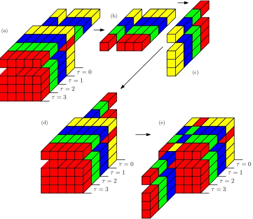
C. Shifting Approach
The delay step (4) in the SMD algorithm can be performed with the reduced parahermitian matrix representation in the
ith iteration by shifting either the k(i)th column or row —
whichever has the greater modified norm according to (7) or (12) — by |τ(i)| coefficients to the zero lag. Elements that are shifted beyond the zero lag, i.e. outside the recorded half-matrix, have to be stored as parahermitian (i.e. Hermitian transposed and time reversed) and appended onto the k(i)th row or column of the shifted matrix at lag-zero. The concate-nated row or column is then shifted by|τ(i)|elements towards
increasingτ.
An example of the shift operation is depicted in Fig. 2 for the case of S(i−1)(z)∈C5×5 with parametersk(i)= 2 and
τ= 3 τ= 2
τ= 1 τ= 0
τ= 3 τ= 2
τ= 1
τ= 0 τ= 0
τ= 1
τ= 2
τ= 3 (a)
(b)
(c)
[image:3.612.313.565.50.269.2](d) (e)
Fig. 2. Example for a matrix where in theith iteration a modified row norm
is maximum: (a) the row is shifted, with non-diagonal elements in thek(i)th
row past the zero lag (b) extracted and (c) parahermitian transposed; (d) these elements are appended to thek(i)th column at zero-lag and (e) shifted in the
opposite direction with all off-diagonal column elements.
τ(i) = −3. Because of the negative sign of τ(i), it is here
the 2nd row that has to be shifted first, followed by the 2nd column shifted in the opposite direction. Note that because the row and column shifts operate in opposite directions , the polynomial in thek(i)th position along the diagonal remains
unaltered. An efficient implementation will therefore exclude this polynomial from otherwise spurious shift operations, as shown in the example of Fig. 2.
D. Truncation and Rotation
Following this shifting procedure, for the 2nd step of the SMD iteration an ordered EVD of the lag-zero matrixS(i)′[0]
is perfomed, yielding the modal matrix Q(i) that has to be applied to all lags 0≤τ≤N(i).
To curb the growth in order of S(i)(z) at every iteration, trimming of matrices S(i)[τ] for outer lag values has been advocated previously [12], [15], [20]. This trimming is based on a thresholdǫapplied to the Frobenius normk ·kF, whereby
S(i)(z)is reduced to an orderN˜(i) such that
kS(i)[τ]kF< ǫ∀τ >N˜(i). (14)
Since Q(i) is unitary, kS(i)[τ]k
F = kS(i)′[τ]kF. Truncation
can therefore be performed onS(i)′(z)prior to the computa-tionally expensive rotation to createS(i)(z).
There is also an option to combine the calculation of the Frobenius norm at the ith iteration with the calculation of column and row norms, which will be required for the parameter search of{k(i+1), τ(i+1)}at the(i+ 1)th iteration.
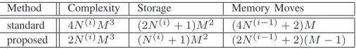
[image:3.612.79.271.51.142.2]TABLE I
APPPROXIMATERESOURCEREQUIREMENTS.
Method Complexity Storage Memory Moves
standard 4N(i)M3 (2N(i)+ 1)M2 (4N(i−1)+ 2)M
proposed 2N(i)M3 (N(i)+ 1)M2 (2N(i
−1)+ 2)(M−1)
therefore is particular advantageous for larger dimensions M
when factorisingR(z)∈CM×M.
E. Reduction in Memory and Computational Cost
The memory required to store the causal part of S(i)(z) at the ith iteration is equal to (N(i) + 1)M2 coefficients, and therefore approximately half of what a full storage needs. During the ith iteration, the first delay step involves
2(N(i−1)+ 1)(M−1)coefficients to be shifted in memory, as
opposed to2(2N(i−1)+ 1)M for a full matrix representation.
Therefore, the number of coefficient moves during the shift step is also halved using the proposed approach.
In terms of multiply-accumulates, the rotation operation with Q(i) during the 2nd step of the ith iteration
re-quires 2M3( ˜N(i)+ 1) MACs, saving more than half of the
operations executed during the standard approach outlined in Sec. II-B. The various aspects of resource requirements are summarised in Tab. I.
Fori≫1, simulations in [15] indicate that the order of the parahermitian matrix S(i)(z) does no longer increase when trimmedafter every iteration. Therefore,
˜
N(i)≈N(i)− |τ(i)| (15)
and the additional cost reduction due to trimming S(i)′(z)
prior to the 2nd iteration step saves an additional 2M3|τ(i)|
MACs.
IV. RESULTS
To benchmark the proposed approach, this section first defines the performance metric for evaluating differently im-plemented SMD algorithms before setting out a simulation scenario, over which an ensemble of simulations will be performed.
A. Performance Metric
Since SMD iteratively minimises off-diagonal energy, a suitable normalised metric defined in [15] is
E(normi) =
P
τ
PM k=1kˆs
(i)
k [τ]k
2 2
P
τkR[τ]k2F
, (16)
which divides the off-diagonal energy at the ith iteration by the total energy. Since the total energy remains unaltered under paraunitary operations, the normalisation is performed by R(z)which can be calculated once, rather than by evaluating S(i)(z) at every iteration. The definition of sˆ(ki)[τ] is given in (7). For a logarithmic metric, the notation 5 log10E
(i) norm
reflects that quadratic covariance terms are squared once more for the norm calculations in (16).
0 0.02 0.04 0.06 0.08 0.1 0.12 0.14 0.16 0.18 0.2
Time / s
-15 -10 -5 0
5l
og1
0
E
{
E
(
i
)
n
o
rm
}
/
[d
B
]
[image:4.612.50.303.78.113.2]proposed,M= 5 standard,M= 5 proposed,M= 10 standard,M= 10
Fig. 3. Diagonalisation metric vs. algorithm execution time for the proposed reduced and standard SMD implementations forM∈ {5; 10}.
B. Simulation Scenario
The simulations below have been performed over an en-semble of 103 instantiations of R(z) ∈ CM×M, M ∈
{5; 10}, based on the randomised source model in [15]. This
source model generates R(z) = ˜U(z)D(z)U(z), whereby the diagonal D(z) ∈ CM×M contains the power spectral
densities (PSDs) of M independent sources. These sources are spectrally shaped by innovation filters such thatD(z)has an order of 120, with a restriction on the placement of zeros to limit the dynamic range of the PSDs to about 30dB. Random paraunitary matrices U(z) ∈ CM×M
of order 60 perform a convolutive mixing of these sources, such thatR(z)has a full polynomial rank and an order of 240.
During iterations, a truncation parameter of µ= 10−6 and
a stopping threshold of ρ = 10−6 were used. The standard
and proposed SMD implementations are run over I = 200
iterations, and at every iteration step the metric defined in Sec. IV-A is recorded together with the elapsed execution time.
C. Diagonalisation
The ensemble-averaged diagonalisation according to (16) was calculated for both the standard and reduced SMD imple-mentation. While both algorithms are functionally identical and exhibit the same diagonalisation performance over algo-rithm iterations, the cost per iteration step for both methods is shown in Fig. 3. The curves demonstrate that for M ∈
{5; 10}, the lower complexity associated with the reduced
SMD implementation translates to a faster diagonalisation than observed for the standard SMD realisation. Using a matrix with a larger spatial dimension of M = 10 versus
M = 5results in poorer diagonalisation for both algorithms, but the same relative performance increase is still seen for the proposed reduced approach.
Iteration
0 20 40 60 80 100 120 140 160 180 200
P
ar
ah
er
m
it
ia
n
m
at
ri
x
or
d
er
20 30 40 50 60 70 80 90
[image:5.612.96.248.57.178.2]before truncation M = 5 after truncation M = 5 before truncation M = 10 after truncation M = 10
Fig. 4. Parahermitian matrix order before and after truncation vs. algorithm iteration for the proposed reduced implementation forM∈ {5; 10}.
the paraunitary matrix as iterations proceed, requiring costly convolutions of paraunitary polynomial matrices. If these pa-raunitary matrices do not need to be extracted, then eliminating the cost for the paraunitary matrix update will widen the performance gap between the methods in Tab. I. Using the Matlab profiler further shows that the execution time for matrix multiplications (i.e., the number of matrix multiplications) has been substantially reduced by the proposed method; while Matlab is optimised for such matrix multiplication, its shifting of memory is as not efficient and dominates the execution time. Despite this, Tab. I indicates a 20% reduction in cost when using the proposed over the standard SMD implementation.
D. Truncation of Parahermitian Matrix
When using the proposed reduced representation, the impact of parahermitian matrix truncation according to (14) on the matrix order can be seen in Fig. 4. Note, the first two iterations have been omitted for clarity. By moving the truncation step to before the rotation stage in the proposed approach, it is clear that a significant number of redundant MAC operations have been avoided.
V. CONCLUSION
The symmetry in the parahermitian matrix has been ex-ploited when calculating a polynomial EVD, which has been exemplified here by a focus on the SMD algorithm. We have proposed a reduced matrix representation which only records its causal part; this approach can produce the same accuracy of decomposition as a standard matrix representation in the SMD algorithm, but with increased efficiency with respect to memory use and computational complexity. Simulation results underline that the same diagonalisation performance can be achieved by both methods, but within a shorter execution time for the approach based on a reduced representation.
When designing PEVD implementations for real applica-tions, the potential for the proposed techniques to reduce complexity and memory requirements therefore offers benefits without deficits w.r.t. important performance metrics such as the diagonalisation of the SMD algorithm. The reduced representation of parahermitian matrices proposed here can be extended to any PEVD algorithm by adapting the shift and rotation operations accordingly.
ACKNOWLEDGEMENT
Fraser Coutts is the recipient of a Caledonian Scholarship; we would like to thank the Carnegie Trust for their support.
REFERENCES
[1] P. P. Vaidyanathan. Multirate Systems and Filter Banks. Prentice Hall, Englewood Cliffs, 1993.
[2] C. Liu, C. H. Ta, and S. Weiss. Joint precoding and equalisation design using oversampled filter banks for dispersive channels with correlated noise. InIEEE Workshop on Signal Processing Systems, pp. 232–236, Shanghai, China, Oct. 2007.
[3] S. Weiss, S. Redif, T. Cooper, C. Liu, P. D. Baxter, and J. G. McWhirter. Paraunitary oversampled filter bank design for channel coding. EURASIP Journal of Applied Signal Processing, 2006. [4] C. H. Ta and S. Weiss. A design of precoding and equalisation for
broadband MIMO systems. In 41st Asilomar Conf. Signals, Systems and Computers, pp. 1616–1620, Pacific Grove, CA, USA, Nov. 2007. [5] S. Redif, J. McWhirter, and S. Weiss. Design of FIR paraunitary filter
banks for subband coding using a polynomial eigenvalue decomposition.
IEEE Transactions on Signal Processing, 59(11):5253–5264, Nov. 2011. [6] M. Alrmah, S. Weiss, and S. Lambotharan. An extension of the music algorithm to broadband scenarios using polynomial eigenvalue decom-position. In19th European Signal Processing Conference, pp. 629–633, Barcelona, Spain, Aug. 2011.
[7] S. Weiss, M. Alrmah, S. Lambotharan, J. McWhirter, and M. Kaveh. Broadband angle of arrival estimation methods in a polynomial matrix decomposition framework. InIEEE 5th Int. Workshop Comp. Advances in Multi-Sensor Adaptive Proc., St. Martin, pp. 109–112, Dec. 2013. [8] A. Alzin, F. Coutts, J. Corr, S. Weiss, I. K. Proudler, and J. A. Chambers.
Adaptive broadband beamforming with arbitrary array geometry. In
IET/EURASIP Intelligent Signal Processing, London, UK, Dec. 2015. [9] S. Weiss, S. Bendoukha, A. Alzin, F. Coutts, I. Proudler, and J.
Cham-bers. MVDR broadband beamforming using polynomial matrix tech-niques. In23rd European Signal Processing Conference, pp. 839–843, Nice, France, Sep. 2015.
[10] Z. Wang, J. G. McWhirter, and S. Weiss. Multichannel spectral fac-torization algorithm using polynomial matrix eigenvalue decomposition. In49th Asilomar Conf. Signals, Systems and Computers, Pacific Grove, CA, Nov. 2015.
[11] I. Gohberg, P. Lancaster, and L. Rodman.Matrix Polynomials. Academic Press, New York, 1982.
[12] J. G. McWhirter, P. D. Baxter, T. Cooper, S. Redif, and J. Foster. An EVD Algorithm for Para-Hermitian Polynomial Matrices. IEEE Transactions on Signal Processing, 55(5):2158–2169, May 2007. [13] P. Vaidyanathan. Theory of optimal orthonormal subband coders.IEEE
Transactions on Signal Processing, 46(6):1528–1543, June 1998. [14] S. Icart, P. Comon. Some properties of Laurent polynomial matrices. In
Conf. Math. Signal Proc., Birmingham, UK, Dec. 2012.
[15] S. Redif, S. Weiss, and J. McWhirter. Sequential matrix diagonalization algorithms for polynomial EVD of parahermitian matrices. IEEE Transactions on Signal Processing, 63(1):81–89, Jan. 2015.
[16] J. Corr, K. Thompson, S. Weiss, J. McWhirter, S. Redif, and I. Proudler. Multiple shift maximum element sequential matrix diagonalisation for parahermitian matrices. In IEEE Workshop on Statistical Signal Pro-cessing, pp. 312–315, Gold Coast, Australia, June 2014.
[17] Z. Wang, J. G. McWhirter, J. Corr, and S. Weiss. Multiple shift second order sequential best rotation algorithm for polynomial matrix EVD. In
Europ. Signal Proc. Conf., pp. 844–848, Nice, France, Sep. 2015. [18] J. Corr, K. Thompson, S. Weiss, J. G. McWhirter, and I. K. Proudler.
Causality-Constrained multiple shift sequential matrix diagonalisation for parahermitian matrices. In Europ. Signal Proc. Conf., pp. 1277– 1281, Lisbon, Portugal, Sep. 2014.
[19] J. Corr, K. Thompson, S. Weiss, I. Proudler, and J. McWhirter. Row-shift corrected truncation of paraunitary matrices for PEVD algorithms. InEurop. Signal Proc. Conf., pp. 849–853, Nice, France, Sep. 2015. [20] J. Foster, J. G. McWhirter, and J. Chambers. Limiting the order of
poly-nomial matrices within the SBR2 algorithm. InIMA Int. Conf. Math-ematics in Signal Processing, Cirencester, UK, Dec. 2006.