Physical water use and water sector activity in environmental input-output analysis

D

EPARTMENT OF

E

CONOMICS

U

NIVERSITY OF

S

TRATHCLYDE

G

LASGOW

PHYSICAL WATER USE AND WATER SECTOR ACTIVITY IN

ENVIRONMENTAL INPUT

-

OUTPUT ANALYSIS

B

Y

OLUWAFISAYO ALABI, MAX MUNDAY, KIM SWALES AND

KAREN TURNER

N

O

16-12

S

TRATHCLYDE

Physical Water Use and Water Sector Activity in Environmental Input-Output Analysis

Alabi, Oluwafisayoa,d_{, Munday, Max} b_{, Swales, Kim}c _{and Turner, Karen}d

a _{Department of Economics, University of Strathclyde, Glasgow, UK,}

b _{Welsh Economy Research Unit (WERU) Cardiff University, UK}

c _{Fraser of Allander Institute (FAI), Department of Economics, University of Strathclyde,}

Glasgow, UK

d _{Centre for Energy Policy (CEP), University of Strathclyde, Glasgow, UK}

Abstract

This paper uses input-output accounting methods to identify the direct, indirect and

induced physical demand for water. Previously the seminal work by Leontief (1970) has

been employed to motivate a fuller account of issues related to sectors that generate and

sectors that clean/treat polluting outputs (Allan et al 2007). The present paper extends this

approach to deal with sectors that use a natural resource and the sector(s) that supply it.

We focus on the case of water use and supply and a case study for the Welsh regional

economy. The analysis shows how the proposed method, using both the quantity

input-output model and the associated price dual, can be used to consider economy wide

implications of the deviation between actual expenditure on the output of the water sector

and actual physical water use. The price paid per physical amount of water appears to vary

greatly amongst different uses. This may occur for various reasons. We argue that such

analysis and information is essential for policy makers and regulators in understanding the

demands on and supply of UK regional water resources, their role in supporting economic

expansion, and can ultimately inform water sustainability objectives and strategies.

Key words:

1. Introduction

Water policies and regulations across the EU (including the water framework directive

WFD) (EU, 2000) provide legislation for planning and delivering better water

environmental management (European Commission, 2011). DEFRA (2011) outlines the

UK’s obligations to deliver under the WFD and also provides wider context in terms of the

uneven geographical distribution of water resources and different levels of stress on the

resources. The UK’s water-stressed regions tend to be more densely populated. Therefore,

future water demands might involve unsustainable water abstraction levels and water stress

in resource abundant regions in order to meet increased demand from more heavily

populated areas. Water companies and regulators therefore face the challenge of

comprehending the complex economic interactions determining water use and the

sustainability of water supply (European Agency, 2015). In particular, there is a need to

appreciate the economy-wide implications of future industry development and how water

use in one industry connects to the embedded water use in supply chains.

This paper investigates the way in which input-output accounting methods can be used to

improve our understanding of the direct, indirect and induced demand for a physical

resource such as water. Conventional environmental input-output modelling attempts to

capture emissions generation, or physical resource use, associated with economic activity.

It does so by linking appropriate direct physical use/output coefficients to standard

(economic) input-output multiplier results. Previously the seminal work by Leontief (1970)

has been employed to motivate a fuller account of issues related to sectors that generate

and sectors that clean/treat polluting outputs (Allan et al. 2007). Specifically, it considers

the resource costs implied by internalising that level of externality that cannot be tolerated,

and who bears them. The present paper extends this approach to deal with sectors that use

a natural resource and the sector(s) that supply it, focusing on water and considering the

resource costs of collecting, preparing and moving water to different types of user.

The paper uses the Welsh Input-Output Tables, together with data from the UK

Environmental Accounts to construct three alternative water multiplier measures for Wales

based around both physical and resource use methods. These produce quantitative results

that differ, sometimes quite radically. The investigation of these differences is important

for both policy and analysis. In this respect the analysis builds on, and extends, the earlier

The remainder of the paper is structured as follows. Section 2 reviews early developments

in environmental input-output modelling. Section 3 gives a step by step account of how

insights from the Leontief (1970) general model can be applied to the demand for, and the

supply of, a physical resource like water. Section 4 describes the data used in this

application and the derivation of adjusted input-output rows that reflect the differences

between payments actually made to the water sector and those implied by actual water use.

Section 5 outlines the main findings of the analysis, focussing on the implications of these

findings for the analysis of water resources within an input-output framework and for

policymakers.

2. Water Resources and Input-Output Framework

The initial application of input-output analysis to the interaction between the economy and

the environment dates back to the 1960s and 1970s. Early models focused on constructing

what Miller and Blair (2009) refer to as “fully integrated models” (Daly, 1968; Isard,

1969). These studies attempted to model both the environmental and economic system in

a manner consistent with the Material Balance Principle (MBP). In this approach, flows

within and between the economy and the environment operate along the same lines as

inter-regional trade in an inter-inter-regional IO model. However, these all-encompassing

economy-environment models were difficult to operationalise.

A second approach is based on the work of Leontief (1970) which discusses the

construction of a “generalised input-output model” that links pollution generation directly

to economic activity and associated cleaning behaviours (Miller and Blair, 2009). This

approach augments the conventional (economic) input-output technical coefficients matrix

with additional rows and columns to reflect pollution generation and abatement activities

by economic sectors. The underlying principle of the Leontief (1970) model identifies

pollution as a by-product of economic activities. This is particularly appropriate for

pollutants whose cost is not internalised by the polluter. Once categorised as a negative

externality, pollution can then be reduced through the operation of abatement sectors

whose activity is at least partly endogenously determined.

More recent applications of environmental output models typically adopt an

economic-ecologic models (see Victor, 1972). They only consider the one-way link between the

economy and the subsequent environmental or resource use implications but do not

explicitly incorporate endogenous cleaning sectors and ecological inputs from the

environment. In this paper we refer to this as the conventional environmental input-output

approach. This method employs both the regular input-output Leontief inverse and a

corresponding vector of direct physical pollutant (or resource use)/output ratios. It has been

commonly applied for allocating responsibility for pollution generation embodied in trade

flows, using multiregional, interregional and international input-output frameworks

(Wiedmann, 2009; Wiedmann et al., 2007). Other applications address natural/physical

resource concerns (Lange, 1998)

This conventional environmental modelling approach has also been used to consider

specific issues around water scarcity and trade (see, for example, Duarte and Yang, 2011).

Dietzenbacher and Velázquez (2007) introduce the concept of ‘virtual water’ to the

input-output literature in considering whether water scarce/abundant regions are likely to be net

importers/exporters of water.1 _{Other authors employ a multi-sectoral attribution to consider}

water allocation problems in and between regions facing acute water scarcity (Carter and

Ireri, 1968; Feng et al. 2007; Guan and Hubacek, 2007; Seung et al. 1997). In this vein

Velázquez (2006) developed an input-output model of industrial water consumption for

Andalusia. This approach permits analysis of the direct and indirect consumption of scarce

water resources allowing the potential for an economic and environmental policy oriented

towards water saving.

Environmental input-output has also provided a framework for consumption accounting

methods for dealing with water use and the estimation of national ‘water footprints’

(Cazcarro, et al., 2010; Chapagain et al., 2006; Hoekstra and Chapagain, 2007; Yu et al.,

2010). Using an illustrative approach, Zhang et al. (2010) show that Chinese water scarcity

issues relate to a disconnect between the geographical distributions of water resources,

economic development and other primary factors of production. This results in a separation

of production and consumption of water-intensive products. These authors use a

multi-regional input-output (MRIO) framework to estimate the nature of virtual water trade and

consumption-based water footprints (see also Okadera et al., 2015). Similarly, White et al.

1 _{The concept of virtual water is the water use embedded, directly or indirectly, in the production of a good or}

(2015) employed an integrated MRIO hydro-economic model to examine a

consumption-based water footprint and the embedded water flows in inter-regional trade in China. They

show that whilst there might be value in increasing imports of virtual water from water rich

regions, care is needed because this could result in greater water stress in other

water-scarce regions.

However, these developments neglect crucial aspects of the Leontief generalised model

approach. These are the internalisation of the negative pollution impacts and the associated

endogenous cleaning activities. There is limited work attempting to apply, discuss and

explore the full Leontief (1970) environmental input-output model (Allan et al., 2007;

Leontief and Ford, 1972).

The Leontief generalised model approach can be usefully applied to water use. It identifies

the economic resources employed in the collection, preparation and movement of water.2

Two specific insights from the operation of the full environmental model prove to be

particularly relevant in this case. First, the resources used in the water supply sector can

act as an alternative index of water use. Second, differences between the water use

multiplier values generated by the conventional environmental and the full Leontief

generalised approach identify important issues for environmental input-output analysis in

particular, but also for input-output analysis as a whole.

3. Method

Tracking water use through the conventional environmental input-output approach,

proceeds in the following way. Sectorally disaggregated output in an economy with n

sectors can be represented as (Miller and Blair, 2009):

[

]

1

q= −I A− f (1)

In equation (1), q and f are respectively the (n x 1) output and final demand vectors, where

the ith element in each respectively is the output and final demand for the product or service

generated by sector i. A is the (n x n) matrix of technical coefficients, where element, aij,

2_{The basic input-output water sector can be thought of as identifying that part of the}

is the value input of sector i directly required to produce one unit of the value output of

sector j.

The

[

I−A

]

−1matrix is the Leontief inverse. Each element,α_{i j,} , gives the output in sector i

directly or indirectly required to produce one unit of final demand in sector j. The sum of

the elements of column j therefore gives the total value of output required, directly and

indirectly, to meet one unit of final demand for the output of sector j. In the application of

the conventional environmental input-output approach to water use, these value multipliers

are transformed into physical water multipliers which measure the physical water required

directly or indirectly to produce a unit of final demand expenditure in each sector. These

are derived as the sum of the conventional column entries in the Leontief inverse, each

weighted by the corresponding industry i’s direct physical water coefficient. This generates

a measure which is the direct and indirect use of physical water per unit value of final

demand. This procedure is represented formally in equation (2).

[

]

1

1 1

p

m =w I−A − (2)

In equation (2) m₁pis a (1x n) row vector, where the ith element is the ith industry’s physical

water multiplier value and w1is a (1 x n) vector where the ith term is the direct physical

water use in sector i, xk,idivided by the total output of sector i, qi,T, so that:

, 1,

,

k i

i i

i T

x w

q

= ∀ (3)

Note that here, as elsewhere, the water sector is denoted as sector k.

Alternatively, the physical water multiplier, ₂p

m , can be calculated using the Leontief

generalised approach. In this case, rather than directly track the physical water use, the

expenditure made on the water supply sector is used to indicate the resources used in

cleaning and delivering water. To identify the direct and indirect water used in meeting a

unit of final demand in sector j, we locate the jth element on the water supply row (the kth

row) of the Leontief inverse and convert this value to physical units by dividing by the

More formally, this is determined by pre-multiplying the Leontief Inverse by a (1 x n) row

vector, w2, where all elements are zero part from the jth, which is the inverse of the average

price of water, 1 k

p− . This generates a (1 x n) row vector of physical water multiplier values,

2 p

m , as:

[

]

1

2 2

p

m =w I−A − (4)

The price of water is found by summing the total expenditure on the output of the water

sector, across all intermediate and final demands taken from the input-output accounts, and

dividing by the total water extracted for these uses.3 _Therefore:

, 1... , ,

, ,

1... ,

k i

i n f k T

k

k i k T i n f

q q p x x = = =

∑

=

∑

(5)

Where the f and T subscripts stand for final demand and total respectively. 4

The multiplier values calculated using the standard environmental IO approach (equation

2) and the Leontief generalised approach (equation 4) are the same if one central

assumptions of the value-denominated input-output analysis holds. This is that all uses of

the output of a particular sector should face the same price for that good or service. In this

specific case, this means that the two multiplier values will be equal if all users of water

face the same price for water. Ifm₁p ≠m₂p, this is because the pattern of physical water use

across sectors does not match the corresponding distribution of expenditure on the output

of the water sector, as captured in the input-output accounts.

Discounting data reporting errors, there are two possible reasons why this might be the

case. First, the technology for abstracting, treating and distributing water might differ

between uses. As Duchin (2009) argues, water itself is a common pool resource that is not

3_{The way in which these physical figures are calculated is given in Section 4 and formalised in equations} (11) to (14).

4 _{An alternative way of calculating}

2 p

m is m₂p =w I₃

[

−A

]

−1where w3 is a (1 x n) row vector where

necessarily directly paid for. In the context of input-output accounts the water sector pays

only for the resources needed to collect/abstract, treat and distribute water but not for the

water itself. The differences in price per unit of physical water delivered could therefore

reflect variations in the value of inputs needed to deliver that water to different uses.

An alternative explanation is that there is some form of price discrimination in the supply

of water to different industries and elements of final demand. This perspective has been

previously applied by Weisz and Duchin (2006) to consider the factors surrounding the

differences between physical and monetary input output analysis in general. It has also

been applied by Allan et al. (2007) in the specific application to the treatment of Scottish

waste.

In the case of Allan et al.’s (2007) analysis of Scottish waste, the production sectors appear

to pay only partially, and unsystematically, for waste treatment, so that, in effect, some

sectors are charged more for waste disposal services than others. For the Welsh water use

analysed in the present paper, all the transactions involve the public water supply and

therefore in principle go through the market mechanism. Therefore in aggregate all the

market resource costs are covered by firms paying for water as an intermediate input and

consumers paying for domestic supply. However, if there is no difference in the resources

needed to supply water to different users, then any difference between the two physical

water multiplier values (m₁pandm₂p) is down to some form of price discrimination.

Whichever explanation applies, if these multiplier values differ, there are prima facie

problems for input-output analysis. If the resources needed to deliver water varies across

uses, and if these are large enough to cause significant variation in the multiplier values,

then there should be greater disaggregation of the input-output table, particularly in this

case the water sector. For example, a disaggregation between the provision of industrial

and domestic water might be appropriate.5 Only if the resources needed to deliver water

are constant in composition across uses but vary in their ability to deliver the same quantity

of water will the conventional environmental input-output multiplier,m₁p, give the correct

value (and the m₂pvalue would give an inaccurate measure).

Alternatively, if price differences solely reflect price discrimination, an appropriate

adjustment can be made to correct the water multiplier calculations. This involves changing

the entries in the water row of the A matrix of the initial input-output accounts to reflect

the true/actual water use. The initial water row vector is therefore replaced by an implied

water row vector derived from multiplying the physical water use per unit of value output

divided by the average price of water.

Again, identifying the water input as the kth row, the resulting vector of multiplier values,

3 p

m

, is given as:

1 *

3 2

p

m =w _I−A _− (6)

In equation (6), elements of the matrix A* are given as the following:

* , , , * , 1, , , ,

i j i j

k i k

k j i k

i T

If i k a a

x p

If i k a w p

q

≠ =

= = = (7)

Under price discrimination, m₃pis the correct water multiplier value.6

This procedure corrects the water multiplier value where price differences represent price

discrimination. It is perhaps important to emphasise that this occurs through revising the

entries in the conventional Leontief inverse. Imagine that there are price variations across

the uses to which a particular product or service - the output of a specific sector - is put. In

this case, a given expenditure is associated with a different physical output of the product,

depending on the use for which that expenditure were made. This also applies to elements

of final demand for water. For example, if exports receive a lower price than output sold

to home consumers, then in increase in household consumption will be associated with a

lower physical output, and a lower actual multiplier impact, than an increase in export

expenditure.

These problems occur whenever such price discrimination is present. Studying a relatively

homogeneous sector, and focussing on the physical output of that sector, more easily

reveals any price differences that exist. Whilst these challenges almost certainly apply in

other sectors, and could be more prevalent with greater product differentiation, they are

likely to be more difficult to detect.

Where the divergence between the relative value and quantity of water used is attributed

to price discrimination, the input-output price model can determine the subsequent

deviation in the prices of all commodities, and therefore the implicit price subsidies or

penalties. The price model is the dual of the quantity model represented by equation (1).

In the original set of input-output accounts the sector prices are calibrated to take unit

values and have the following form:

1

T

i=_I−A _− v (8)

where i is a (n x1) vector of ones, (1-AT₎-1 _{is the Leontief price multiplier and v is the vector}

of unit value added figures in the initial period. Equation (9) gives the corresponding set

of prices,

p

₃p, where the original A matrix is replaced by the augmented A* matrix.

1 * 3

p T

p =_I−A _− v (9)

This is the vector of prices that would hold if all sectors and final demand uses of water

were charged at the same price. Adopting the price model allows the estimation of changes

in relative prices across sectors that demand water services as inputs for production.

Equation (10) calculates these changes ∆p₃p as the vector of percentage price variations:

3 3 100

p p

p p i

∆ =_ − ×_ (10)

If the payment for the services of the water sector were always proportional to the physical

amount of water purchased, then the multiplier values generated using equations (2) (4)

and (6) would be the same, i.e.

m

₁p

=

m

₂p

=

m

₃p and each element of the ₃p

p

be 0. However, this is not the case using the Welsh data. These results are discussed in

some detail in Section 5.

4. Data and derivation of adjusted input-output row entries for actual and implied

water use

This paper uses data relating to the public water supply sector in Wales, which is a

devolved region of the United Kingdom. The input-output accounts are for 2007, the latest

date for which the Welsh input-output table is available (Jones et al., 2010). These accounts

identify the purchases and sales of 88 separately defined industrial sectors, one of which is

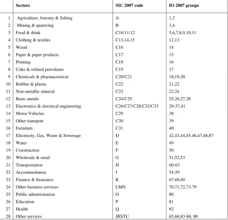
water supply. Some aggregation of these sectors is required to make them consistent with

the data that are available on the industrial use of water resources. Table A1 in the

Appendix reveals the industrial aggregation used in this paper and how the 88 sectors in

the Welsh input-output framework are mapped on to the 27 industries for which water

consumption data are available.

Whilst the input-output data are Welsh specific, information on the physical water use has

to be estimated by spatially disaggregating the English and Welsh Environmental

Accounts. These provide information on industrial and household water use (public water

supply) together with water companies’ leakages in England and Wales for 2006-07.7 From

the outset it is important to say that this disaggregation is made primarily on the assumption

that the intensity of water use across industries and for households do not differ between

England and Wales. In so far as this is not true, the Welsh physical water use figures will

contain inaccuracies.

The vector of Welsh industrial water use is calculated in the following way. Each element

is determined by dividing the England and Wales water use figure in each industry in

proportion to the corresponding industry’s employment levels in the two regions. That is

to say:

, ,

W

W E W i

k i k i E W

i e x x e + +   = _{ }

  (11)

In equation (11), xk,i is the use of water in physical terms in industry i, (industry k is the

water industry), ei is employment in industry i, and the W and E superscripts apply to Wales

and England respectively.

The Welsh household physical water use, xW_{k h,} , is estimated based on the Welsh share of

the England and Wales population (PopW_/PopE+W_{). This is given as:}

, ,

W

W E W

k h k h E W

Pop x x Pop + +   = _{ }

  (12)

However, there is limited information on physical water supplied to all non-household final

demand uses,xW_{k nh,} . This is essentially export demand for Welsh water from England. The

assumption is made that the physical share of non-household water output to the physical

total output is equal to the value share of non-household final demand to the value of all

Welsh water output, as given in the Welsh input-output tables. This corresponds to the

assumption that all non-household final demand uses pay the industry average price for the

water that they purchase, so that:8

, ,

, , ,

, ,

W W

k nh k nh

W W W

k nh W W k h k i

i

k T k nh k

q q

x x x

q q p

 _{  }

=_{  } + _=

− _{ }

 

 

∑

(13)

Total physical Welsh water generation, ,

W k T

x , is the sum of the values calculated using

equations (11), (12) and (13):

, , , ,

W W W W

k T k i k h k nh

i

x =

∑

x +x +x (14)

Using these procedures total Welsh water production in 2007 (public water supply) is

estimated at 253 million cubic metres, of which households accounted for 158 million

(63%) and 69 million cubic metres (27%) were supplied to Welsh industries as

intermediate inputs.

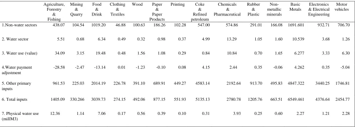
Table 1 presents a condensed version of the 2007 Input-Output Tables for Wales, together

with a number of additions. It shows the pattern of sales of the water sector, the physical

use of water and the accounting adjustments required if expenditure on water is to match

water use. Rows 1 to 6 give accounting data, measured in £ million, 2007 prices. Row 7

gives the physical water use, measured in millions of cubic metres, calculated as discussed

in equations (11) to (14).

Rows 1 and 2 disaggregate the expenditures on domestic output made by industrial sectors

and final demand. Row 1, labelled “Non-water sectors” are the payments made to the

combined non-water sectors; that is, sectors 1-17 and 19-28 (see Table A1). The entries in

row 2, ‘Payments to water sector’ give the payments entry for water services in the original

input-output accounts. The total output of the water sector, at £697.82 million, is just less

than 0.5% of the total Welsh output, which in 2007 is £140,916 million. Note that actual

payments for water are dominated by final demand and particularly household demand

which, at £512.42 million, makes up over 73% of the total. The expenditure on water as an

intermediate input is highest for the ‘Chemicals & Pharmaceuticals’, ‘Public

Administration’, ‘Basic Metals’ and ‘Accommodation’ sectors. Each of these Welsh

sectors spent more than £10 million on water in 2007, the highest being Chemicals &

Pharmaceuticals, at £13.29 million.

Row 3 reports the actual water use, measured in value terms. That is to say, it takes the

physical water use figure from row 7 of Table 2 and multiplies this by the average price of

water. The figure in row 3 is therefore the expenditure for water in its different uses that

would be made if water had the same price in all uses. Note that rows 2 and 3 have the

same row totals, but that the entries for individual uses differ, sometimes by a very large

amount. To begin, the actual use of water as an intermediate input is measured as £190.01

million, over 66% higher than the actual payment for water as an intermediate. The

household use indicates an equal, and opposite, position: household water payments are

greater than the value of water use. For the adjusted water use by individual sectors, six

‘Agriculture, Forestry & Fishing’, ‘Food & Drink’, ‘Accommodation’, ‘Health’, ‘Other

Business Services’ and ‘Chemicals & Pharmaceuticals’.

The figures in row 4, ‘Additional payment for water’ are the differences between the

unadjusted (row 2) and adjusted (row 3) water payment entries. The row total is zero, so

that overpayments are just balanced by underpayments. Where the entries are positive in

this row, it implies an overpayment for water. This occurs for the household consumption

but also for some industrial sectors, such as Coke & Refined Petroleum, ‘Chemicals &

Pharmaceuticals’, ‘Basic Metals’, ‘Construction’, and ‘Public Administration’. These

include some sectors (‘Chemicals and Basic Metals’) which are identified in previous

analysis as high users of water per £ of Welsh GVA (Jones and Munday, 2011).9 A negative

row 4 entry shows that in the unadjusted system these sectors are net under payers. Of the

28 industrial sectors, 19 sectors are net under payers and with ‘Agriculture, Forestry &

Fishing’, ‘Food & Drink’, ‘Education’ and ‘Health’ being responsible for over three

quarters of this underpayment.

Rows 5 and 6 give the other primary inputs and total (unadjusted) value of inputs figures

for each sector from the original Welsh table. The other primary inputs include payments

for labour and other value added, together with imports (from both the rest of the UK and

the rest of the World), taxes and subsidies. For each sector, the unadjusted value of inputs

figure is also the value of output figure.

If the differences in the cost of water for different uses solely reflect price discrimination,

the negative or positive row 4 entries indicate whether any given sector is directly

subsidising water use in other parts of the economy or is being subsidised. As well as

looking at the relative expenditure by individual production sectors, it is also important to

identify the position relative to final demand uses. There are limitations here because for

all non-household final demand sectors the assumption has been imposed, in the face of

insufficient physical water use data, that these sectors fully pay for their water use, hence

their zero value in row 4. However, the household sector’s additional payment entry, which

is based on actual data, has a high positive value £75.76 million, suggesting that households

pay much more for water than their physical water use implies and are subsidising

industrial water use, taken as a whole.

5. Application to Analysis of Industrial Water Use in Wales

In this section we use the Welsh data outlined in Section 4 to calculate the water multiplier

values

m

₁p,

m

₂p and

m

₃pgiven by equations (2), (4) and (6) in Section 3. We also use the equations (8), (9) and (10) to measure the price impacts from imposing a uniform pricing

for Welsh water.

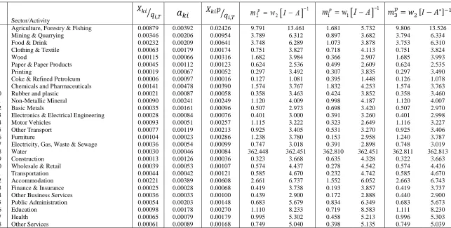
5.1 Physical water multiplier values

Table 2 presents the Type I and Type II values for the three physical water multipliers (

m

₁p

,

m

₂pand

m

₃p) outlined in Section 3. Also reported are the direct water coefficients required to calculate these multipliers. The first data column gives the physical water use coefficient

(xk,i/qi,T), measured in thousands of cubic meters per £ million of output. These figures

comprise the elements of the vector w1. On this measure, the four most water intensive

sectors, in descending order, are ‘Agriculture, Forestry & Fishing’, ‘Mining & Quarrying’,

‘Food & Drink’ and ‘Accommodation’. All of these sectors have a water intensity value

over 2 thousand cubic meters of water per £ million of output. The ‘Agriculture, Forestry

& Fishing’ value at 8,790 cubic meters is particularly high.

The second data column reports the corresponding original direct water coefficient in the

A matrix. These figures give the proportion of total costs in that sector going directly to

the water sector. Using this metric, the top four most water intensive sectors are:

‘Chemicals & Pharmaceuticals’, ‘Agriculture, Forestry & Fishing’, ‘Accommodation’ and

‘Non-Metallic Mineral’. It is clear that ordering the sectors by the share of costs which go

to intermediate water expenditure differs from ordering by the physical water-use intensity.

The third column gives the adjusted expenditure coefficients calculated by multiplying the

physical coefficients in column 1 by the price of water and dividing by a thousand. These

are the water row coefficients used in the A* matrix incorporated in the Leontief inverse

in column 1 but a comparison of columns 2 and 3 indicates the extent to which the two

water intensity measures differ.

For most industries, the adjusted coefficient is greater than the coefficient in the original

input-output table. This is a corollary of the fact that the input-output accounts measure

industrial expenditure to be less, and household expenditure to be more, water intensive

than the physical figures. The four sectors with the biggest difference in absolute terms

between the adjusted and initial water coefficients are, again in decreasing order:

‘Agriculture, Forestry & Fishing’, ‘Mining & Quarrying’, ‘Food & Drink’ and ‘Furniture’.

In all these sectors, the actual payment is lower than the amount of water used, valued at a

constant price. These adjustments are valued at 2.03%, 0.7%, 0.4% and 0.2% respectively

of the total costs for these sectors. The four sectors which have the biggest negative

difference between their adjusted and actual water payment are ‘Chemicals &

Pharmaceuticals’, Coke & Refined Petroleum, ‘Basic Metals’ and ‘Public Administration’.

This indicates that these sectors are paying more for their water use than would be expected

from the physical figures. However, these values are much smaller, at 0.09%, 0.08%,

0.06% and 0.05% of total costs respectively.

The figures in columns 4 and 5 give the physical water Type I and Type II multiplier values

using the conventional environmental input-output approach,

m

₁p, as given in equation (2). They are measured in thousand cubic meters for each £million of final demand expenditure.

The Type I multipliers include only direct and indirect effects. That is to say, in measuring

Type I multipliers household consumption is held constant and only endogenous

intermediate water demands are included as elements of the supply chain. It is Type I

multipliers that are typically used for footprint analysis. Type II multipliers also

incorporate the induced water consumption of direct workers, and also those workers

attributed to the sectors extended supply chain. This would be the most appropriate

multiplier value for increases in activity which were expected to be accompanied by

increases in population.

The conventional Type I physical water multiplier value presented in column 4 must be

higher than the corresponding direct water coefficient shown in column 1, because it

incorporates both the direct water input and the embedded water in the other intermediate

cubic meters per £1 million final demand whereas the conventional Type I value is 9,790

cubic meters. Typically, the difference is relatively small but in some cases the

proportionate differences can be large. The ‘Food & Drink’ sector has a direct water

coefficient of 2,320 cubic meters but a Type I multiplier value 60% higher at 3,790 cubic

meters per £ million of final demand.

The conventional physical Type II water multiplier values are higher still, as they

incorporate additional induced household water use. The Type II measure used

endogenises all the household water use, which is more than double intermediate water

use. Therefore, the Type II physical water multiplier is significantly higher than the Type

I value for most sectors. Although the ‘Agriculture, Forestry & Fishing’ sector maintains

its position as the most water intensive on this measure, other, more labour intensive,

sectors begin to play a more prominent role. ‘Education’ moves from 1,110 cubic meters

on the Type I multiplier to 8,230 cubic meters for the Type II and takes second place on

that measure. ‘Accommodation’ shows a similarly large gain moving from the Type I to

Type II multiplier measure and at 6,740 cubic meters per £1 million final demand is the

third most water intensive sector.

The Type I and Type II physical water multiplier values calculated on the basis of water

sector payments are shown in columns 6 and 7. Note first the low value for the Type I

multiplier values. For 20 industries the Type I

m

₂p multiplier value is lower than the

corresponding

m

₁pfigure. The Type I

m

₂p multiplier value is never greater than 2,000 cubic meters per £1million and in only five sectors is it greater than 1,000 cubic meters per £1

million. ‘Chemicals & Pharmaceuticals’ has the largest value, at 1,830 cubic meters,

followed by ‘Agriculture, Forestry & Fishing’, ‘Accommodation’, ‘Food & Drink’ sectors.

The relative low measure stems from the lower expenditure on water as an intermediate

input than would be expected from the physical water use.

The Type II values incorporate household water use which is overvalued in the expenditure

(as against physical) figures. This means that there is no overall bias in the Type II

m

₂p

value but there are big differences in the Type II

m

₁pand

m

₂pvalues for some individual sectors. Examples are ‘Agriculture Forestry & Fishing’, ‘Mining & Quarrying’, ‘Food &

The

m

₃pmultiplier adjusts the Leontief inverse so that the technical water expenditure coefficients match the physical intermediate and final demand water use values. If the

adjusted A matrix is used, the conventional and the extended Leontief multiplier values

into line, so thatw₁_1−A*_−1=w₂_1−A*_−1. This is the appropriate procedure if the

mismatch between the physical and expenditure water use data is solely due to price

discrimination amongst water uses. In this case it is clear that the

m

₃p values are much

closer to those for

m

₁pthan to those for

m

₂p. This suggests that calculating the physical water multipliers by just tracking the value of output of water sector will give potentially very

inaccurate multiplier values for some individual sectors. On the other hand, the

conventional environmental approach, which augments the value Leontief inverse with

direct physical water/output ratios generates multiplier estimates which, whist theoretically

incorrect, are extremely close to the

m

₃p values. However, this almost certainly reflects the small scale of the water sector in the Welsh economy. Adjusting the coefficients for a large

sector should have bigger impacts on the calculated inverse values.

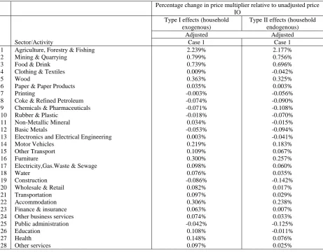
5.2 Price multipliers

If the variation across uses in the price paid per unit of delivered physical water is the result

of pure price discrimination, then the impact on commodity prices of adjusting the water

payments for the actual direct water use can be calculated using equations (8), (9) and (10).

The deviations from the original prices are given in Table 3. These figures show whether

sectors at present bear the full resource cost (or not) of water use through direct and/or

knock on impacts on the price of their output. Column 1 reports the impacts on the prices

of sectoral output using the Type I price multiplier values and the adjusted system. In this

case wage payments are taken as an element of the value added vector, v, and do not adjust

to variations in the sector prices; the nominal wage is held constant. The percentage change

in prices in column 2 identify the corresponding results using Type II multipliers.

Essentially this holds the real wage constant and adjusts the nominal wage to changes in

sector prices. An important issue here is that the price consumers pay for water is above

the average price so that an adjustment to uniform pricing will have a direct impact on the

In the Type I case there are 7 sectors where the price of output would be lower if a uniform

price is charged for water across all uses. The largest negative adjustments are for the

‘Construction’, ‘Coke & Refined Petroleum’ and ‘Chemicals & Pharmaceuticals’ sectors.

However, these impacts are small. These sectors all suffer a cost disadvantage of less than

0.1% stemming from the existing water price differentials. In 21 sectors the adjustment

increases the Type I price multiplier values. In some cases, the impact is particularly high,

with the ‘Agriculture, Forestry & Fishing’ price increasing by 2.24% and prices in the

‘Mining & Quarrying’, and ‘Food & Drink’ sectors rising by 0.80% and 0.74%

respectively.

In calculating the Type II adjusted prices, two changes to the Type I method are made.

First wage income is removed from the vector of sectoral value added, so that all elements

in the value added vector are reduced. Second, the A matrix is augmented to incorporate

the wage and household expenditure. The net impact is to reduce the adjusted price in all

sectors as against the Type I value. That is to say, if with the Type I multiplier the price

adjustment was negative, it is even more negative with the Type II calculation. On the other

hand, if the Type I price change is positive, the Type II value will be smaller, or even

negative.

The biggest difference occurs for Education. Row 4 in Table 3 shows that Education is a

net under-payer for water. This is reflected in the higher Type I price multiplier in the first

column of Table 7. However, Education is a labour/wage intensive sector. This means that

in the Type II case it is impacted by the effect of households over-paying for water as an

“input” to provision of labour services. In the adjusted system, on the other hand, where

households only pay the unit cost for the water they actually use, this puts downward

pressure on the cost of labour and on the price multipliers of labour-using sectors.

6. Conclusions

This paper explores alternative input-output approaches to generating physical multiplier

values using Welsh water data. In particular, it compares the results from using the

conventional physical environmental input-output model with an approach based upon an

earlier generalised Leontief (1970) method, both with and without adjustments to the A

matrix. Essentially the generalised Leontief method uses the demand for the output of the

physical water use. The motivation for using this alternative approach came from the

importance attached in Leontief (1970) for cleaning sectors. However, in many other cases

the physical use of environmental goods, such as rare metals, could be tracked by the

expenditures on the industries supplying such goods.

In the case of Welsh water, the generalised Leontief model works very badly. This is

because the price paid per physical amount of water appears to vary greatly amongst

different uses. In general, the data suggest water used for household consumption is

charged at a higher price than for intermediate industrial demand. There is also a wide price

variation across different industries. Only if physical water-use data are employed to adjust

the input-output A matrix does the generalised Leontief model work satisfactorily. In

principle this is problematic for input-output analysis in general. However, the small scale

of the Welsh water sector means that in actual fact, the conventional environmental

input-output multipliers appear to be quite accurate.

In terms of implications for policy, they key issue is that accurate physical water multiplier

values are required in order to calculate the impact of industrial development strategies on

the demand for water and therefore the sustainability of growth. The major policy

implication of this work for Wales is that water expenditure information reported in the

core economic input-output accounts is inadequate for producing accurate physical water

multiplier values. This implies that the tables must be augmented with direct physical water

coefficients. However, physical data on resource use and physical data (often referred to

as environmental satellite accounts) are commonly not available, particularly at a regional

level. Section 4 has explained that Welsh specific physical water coefficients are

unavailable so that averages across a wider ‘England and Wales’ region have had to be

References

Allan, G., McGregor, P.G., Swales, J.K., and Turner, K., 2007. Impact of alternative electricity generation technologies on the Scottish economy: an illustrative input-output analysis.

Proceedings of the Institution of Mechanical Engineers, Part A: Journal of Power and Energy, 221 (2), 243–254.

Allan, G.J., Hanley, N.D., Mcgregor, P.G., Kim Swales, J., and Turner, K.R., 2007. Augmenting the input--output framework for common pool resources: operationalising the full Leontief environmental model. Economic Systems Research, 19 (1), 1–22.

Carter, H.O. and Ireri, D., 1968. Linkage of California-Arizona input-output models to analyze water transfer patterns. University of California, Department of Agricultural Economics.

Cazcarro, I., Pac, R.D., and Sánchez-Chóliz, J., 2010. Water consumption based on a disaggregated Social Accounting Matrix of Huesca (Spain). Journal of Industrial Ecology, 14 (3), 496–511.

Chapagain, A.K., Hoekstra, A.Y., Savenije, H.H.G., and Gautam, R., 2006. The water footprint of cotton consumption: An assessment of the impact of worldwide consumption of cotton products on the water resources in the cotton producing countries. Ecological Economics, 60 (1), 186–203.

Daly, H.E., 1968. On economics as a life science. The Journal of Political Economy, 392–406.

Defra (2011) 'Water for Life' (See https://www.gov.uk/government/publications/water-for-life)

Dietzenbacher, E. and Velázquez, E., 2007. Analysing Andalusian Virtual Water Trade in an Input– Output Framework. Regional Studies, 41 (January 2015), 185–196.

Duarte, R. and Yang, H., 2011. Input–Output and Water: Introduction To the Special Issue.

Economic Systems Research, 23 (January 2015), 341–351.

Duchin, F., 2009. Input-output economics and material flows. In: Handbook of input-output economics in industrial ecology. Springer, 23–41.

Environmental Agency (2015) 2010 to 2015 Government Policy: Water Industry (See

https://www.gov.uk/government/publications/2010-to-2015-government-policy-water-industry) European Union (2011) Blueprint to safeguard Europe’s water resources (See

http://www.eea.europa.eu/policy-documents/a-blueprint-to-safeguard-europes

EU Water Framework Directive (2000). See http://ec.europa.eu/environment/water/water-framework/index_en.html

Feng, S., Li, L.X., Duan, Z.G., and Zhang, J.L., 2007. Assessing the impacts of South-to-North Water Transfer Project with decision support systems. Decision Support Systems, 42 (4), 1989– 2003.

Guan, D. and Hubacek, K., 2007. Assessment of regional trade and virtual water flows in China.

Ecological Economics, 61 (1), 159–170.

Hoekstra, A.Y. and Chapagain, A.K., 2007. Water footprints of nations: water use by people as a function of their consumption pattern. Water resources management, 21 (1), 35–48.

Isard, W., 1969. Some notes on the linkage of the ecologic and economic systems. Papers in Regional Science, 22 (1), 85–96.

Lange, G.-M., 1998. Applying an integrated natural resource accounts and input--output model to development planning in Indonesia. Economic Systems Research, 10 (2), 113–134.

Leontief, W., 1970. Environmental repercussions and the economic structure: an input-output approach. The review of economics and statistics, 262–271.

Leontief, W. and Ford, D., 1972. Air pollution and the economic structure: empirical results of input-output computations. Input-output techniques, 9–30.

Miller, R.E. and Blair, P.D., 2009. Input-Output Analysis: Foundations and Extensions. Cambridge University Press.

Okadera, T., Geng, Y., Fujita, T., Dong, H., Liu, Z., Yoshida, N., and Kanazawa, T., 2015. Evaluating the water footprint of the energy supply of Liaoning Province, China: A regional input–output analysis approach. Energy Policy, 78, 148–157.

Seung, C.K., Harris, T.R., and MacDiarmid, T.R., 1997. Economic impacts of surface water reallocation policies: A comparison of supply-determined SAM and CGE models. Journal of Regional analysis and Policy, 27, 55–78.

Velázquez, E., 2006. An input–output model of water consumption: Analysing intersectoral water relationships in Andalusia. Ecological Economics, 56 (2), 226–240.

Victor, P.A., 1972. Pollution: economy and environment.

Weisz, H. and Duchin, F., 2006. Physical and monetary input--output analysis: What makes the difference? Ecological Economics, 57 (3), 534–541.

White, D.J., Feng, K., Sun, L., and Hubacek, K., 2015. A hydro-economic MRIO analysis of the Haihe River Basin’s water footprint and water stress. Ecological Modelling.

Wiedmann, T., 2009. A review of recent multi-region input–output models used for consumption-based emission and resource accounting. Ecological Economics, 69 (2), 211–222.

Wiedmann, T., Lenzen, M., Turner, K., and Barrett, J., 2007. Examining the global

environmental impact of regional consumption activities - Part 2: Review of input-output models for the assessment of environmental impacts embodied in trade. Ecological Economics, 61, 15–26.

Yu, Y., Hubacek, K., Feng, K., and Guan, D., 2010. Assessing regional and global water footprints for the UK. Ecological Economics, 69 (5), 1140–1147.

[image:25.842.57.787.122.384.2]

Table 1. The conventional and full Leontief environmental Wales industry-by-industry (28x28) IO table for 2007 (£million, condensed) Agriculture, Forestry & Fishing Mining & Quarry Food & Drink Clothing & Textiles

Wood Paper & Paper Products

Printing Coke & Refined petroleum Chemicals & Pharmaceutical Rubber & Plastic Non-metallic minerals Basic Metals Electronics & Electrical Engineering Motor vehicles

1.Non-water sectors 438.07 104.54 1019.20 46.88 100.63 186.26 102.28 547.00 574.86 291.01 166.08 1691.601 932.71 706.70

2. Water sector 5.51 0.68 6.34 0.49 0.32 0.98 0.37 4.99 13.29 1.05 1.60 10.539 3.68 1.26

3. Water use (value) 34.09 3.15 19.48 0.48 1.56 1.08 0.29 0.84 10.84 0.70 1.65 6.277 3.33 6.30

4.Water payment adjustment

-28.58 -2.47 -13.14 0.01 -1.23 -0.10 0.08 4.15 2.44 0.35 -0.06 4.262 0.35 -5.04

5. Other primary inputs

961.53 225.03 2014.19 226.78 391.10 689.91 449.27 4583.14 2192.64 913.70 495.83 4847.322 3440.25 1746.81

6. Total inputs 1405.09 330.266 3039.73 274.15 492.06 877.15 551.93 5135.13 2780.78 1205.76 663.51 6549.461 4376.64 2454.77

7. Physical water use (millM3)

[image:26.842.39.812.161.429.2]

Table 1 Continued

Other

transport Furniture

Electricity gas, waste &

sewage

Water Construction

Wholesale & Retail

Transportation Accommodation Finance & Insurance

Other business services

Public Adminis

tration

Education Health Other services

1. Non-water sectors 535.79 192.01 2543.56 480.89 1690.98 1986.40 933.10 575.50 1154.37 1771.42 1434.40 538.05 2957.29 720.43

2. Water sector 2.70 0.21 2.86 0.32 6.41 4.55 1.54 10.21 1.09 4.167 12.89 6.51 6.46 3.23

3. Water use (value) 4.83 2.63 5.22 0.58 1.84 9.22 4.41 15.97 2.66 12.601 9.38 9.85 14.64 6.11

4. Water payment

adjustment -2.13 -2.42 -2.35 -0.26 4.57 -4.67 -2.86 -5.77 -1.57 -8.433 3.50 -3.34 -8.18 -2.88 5. Other primary

inputs 1723.80 728.80 2734.05 216.6 3401.78 6590.29 2719.96 2039.37 2744.31 10776.20 4899.40 3107.50 5198.50 2908.28

6. Total inputs 2262.29 921.01 5280.48 697.82 5099.17 8581.27 3654.61 2625.09 3899.78 12551.80 6346.70 3652.10 8162.2 3631.94

7. Physical water use

[image:27.842.62.793.114.385.2]

Table 1 Continued

Total Intermediate

Demand

Households Tour 1-3 Tour 4+ Tour Intl

Tour

Bus Government GFCF Stock2007

Exports RUK

Exports ROW

Total Final Demand

Total Demand Products

1.Non-water sectors 24055.12 18731.33 217.37 964.26 296.33 217.03 13785.90 3003.90 498.60 25840.20 8828.40 72382.90 140219.10

2. Water sector 114.26 512.42 0.14 0.63 0.17 0.15 0.00 15.44 38.56 15.23 0.84 583.56 697.82

3. Water use (value) 190.01 436.66 0.14 0.63 0.17 0.15 0.00 15.44 38.56 15.23 0.84 507.81 697.82

4. Water payment

adjustment -75.76 75.76 0.00 0.00 0.00 0.00 0.00 0.00 0.00 0.00 0.00 75.76 0.00

5. Other primary inputs 273.40 17639.60 26.20 159.50 41.90 28.20 481.70 2413.10 189.30 5448.10 1382.20 27809.81 100776.20

6. Total inputs -33.90 36883.4 243.70 1124.40 338.40 245.40 14267.60 5432.40 726.50 31303.50 10211.10 100776.20 198278.90

7. Physical water use

[image:28.842.89.732.146.471.2]

Table 2. Water Use in Wales in 2007 in thousand Cubic Meters (1000M3₎

Sector/Activity

1 Agriculture, Forestry & Fishing 0.00879 0.00392 0.02426 9.791 13.461 1.681 5.732 9.806 13.526 2 Mining & Quarrying 0.00346 0.00206 0.00954 3.789 6.312 0.897 3.682 3.794 6.334 3 Food & Drink 0.00232 0.00209 0.00641 3.748 6.289 1.073 3.878 3.753 6.310 4 Clothing & Textile 0.00063 0.00179 0.00174 0.751 3.827 0.718 4.113 0.751 3.824 5 Wood 0.00115 0.00066 0.00316 1.682 3.984 0.366 2.907 1.685 3.993 6 Paper & Paper Products 0.00045 0.00112 0.00123 0.624 2.536 0.499 2.609 0.624 2.535 7 Printing 0.00019 0.00067 0.00052 0.297 3.492 0.307 3.835 0.297 3.490 8 Coke & Refined Petroleum 0.00006 0.00097 0.00016 0.127 1.081 0.395 1.448 0.126 1.078 9 Chemicals and Pharmaceuticals 0.00141 0.00478 0.00390 1.574 3.767 1.832 4.253 1.574 3.763 10 Rubber and plastic 0.00021 0.00087 0.00058 0.358 3.463 0.424 3.852 0.358 3.460 11 Non-Metallic Mineral 0.00090 0.00241 0.00249 1.120 4.009 0.998 4.187 1.120 4.007 12 Basic Metals 0.00035 0.00161 0.00096 0.507 2.973 0.698 3.420 0.507 2.970 13 Electronics & Electrical Engineering 0.00028 0.00084 0.00076 0.401 3.000 0.391 3.260 0.401 2.998 14 Motor Vehicles 0.00093 0.00051 0.00257 1.115 3.222 0.323 2.649 1.116 3.227 15 Other Transport 0.00077 0.00119 0.00213 0.925 3.405 0.531 3.270 0.925 3.406 16 Furniture 0.00104 0.00023 0.00286 1.238 3.780 0.153 2.958 1.240 3.787 17 Electricity, Gas, Waste & Sewage 0.00036 0.00054 0.00099 0.747 3.018 0.391 2.898 0.748 3.019 18 Water 0.00030 0.00046 0.00084 362.448 362.451 362.810 362.451 362.811 362.813 19 Construction 0.00013 0.00126 0.00036 0.323 3.668 0.635 4.328 0.322 3.663 20 Wholesale & Retail 0.00039 0.00053 0.00107 0.574 4.437 0.278 4.542 0.574 4.436 21 Transportation 0.00044 0.00042 0.00121 0.585 4.670 0.232 4.742 0.585 4.670 22 Accommodation 0.00221 0.00389 0.00608 2.661 6.737 1.552 6.052 2.663 6.743 23 Finance & Insurance 0.00025 0.00028 0.00068 0.419 3.738 0.193 3.857 0.419 3.737 24 Other Business Services 0.00036 0.00033 0.00100 0.439 2.900 0.172 2.888 0.440 2.900 25 Public Administration 0.00054 0.00203 0.00148 0.683 5.679 0.834 6.349 0.683 5.673 26 Education 0.00098 0.00178 0.00270 1.110 8.233 0.719 8.583 1.111 8.230 27 Health 0.00065 0.00079 0.00179 0.995 5.302 0.458 5.213 0.996 5.303 28 Other Services 0.00061 0.00089 0.00168 0.749 5.040 0.398 5.135 0.749 5.039

𝑋𝑋𝑘𝑘𝑘𝑘 _𝑞𝑞 𝑘𝑘,𝑇𝑇

� 𝑋𝑋𝑘𝑘𝑘𝑘𝑝𝑝 _𝑞𝑞 𝑘𝑘,𝑇𝑇

�

[image:29.595.77.539.121.481.2]

Table 4. Impact on Output Prices of the adjustment to full Leontief environmental IO accounts

Percentage change in price multiplier relative to unadjusted price IO

Type I effects (household exogenous)

Type II effects (household endogenous)

Adjusted Adjusted

Sector/Activity Case 1 Case 1

1 Agriculture, Forestry & Fishing 2.239% 2.177%

2 Mining & Quarrying 0.799% 0.756%

3 Food & Drink 0.739% 0.696%

4 Clothing & Textiles 0.009% -0.042%

5 Wood 0.363% 0.325%

6 Paper & Paper Products 0.035% 0.003%

7 Printing -0.003% -0.056%

8 Coke & Refined Petroleum -0.074% -0.090%

9 Chemicals & Pharmaceuticals -0.071% -0.108%

10 Rubber & Plastic -0.018% -0.070%

11 Non-Metallic Mineral 0.034% -0.015%

12 Basic Metals -0.053% -0.094%

13 Electronics and Electrical Engineering 0.003% -0.041%

14 Motor Vehicles 0.219% 0.183%

15 Other Transport 0.109% 0.067%

16 Furniture 0.300% 0.257%

17 Electricity,Gas.Waste & Sewage 0.098% 0.060%

18 Water 0.076% 0.035%

19 Construction -0.086% -0.142%

20 Wholesale & Retail 0.082% 0.017%

21 Transportation 0.097% 0.029%

22 Accommodation 0.306% 0.238%

23 Finance & insurance 0.063% 0.007%

24 Other business services 0.074% 0.033%

25 Public administration -0.042% -0.125%

26 Education 0.108% -0.011%

27 Health 0.148% 0.076%

[image:30.595.67.520.111.548.2]

Table A1. Production Sectors/Activities Identified in the Wales Water IO Tables, 2007

Sectors SIC 2007 code IO 2007 groups

1 Agriculture, forestry & fishing A 1,2

2 Mining & quarrying B 3,4

3 Food & drink C10/11/12 5,6,7,8,9,10,11 4 Clothing & textiles C13,14,15 12,13

5 Wood C16 14

6 Paper & paper products C17 15

7 Printing C18 16

8 Coke & refined petroleum C19 17 9 Chemicals & pharmaceutical C20/C21 18,19,20

10 Rubber & plastic C22 21,22

11 Non-metallic mineral C23 23,24

12 Basic metals C24/C25 25,26,27,28

13 Electronics & electrical engineering C26/C27/C28/C32/C33 29-37,41

14 Motor Vehicles C29 38

15 Other transport C30 39

16 Furniture C31 40

17 Electricity, Gas, Waste & Sewerage D 42,43,44,45,46,47,48,87

18 Water E 49

19 Construction F 50

20 Wholesale & retail G 51,52,53

21 Transportation H 60-63

22 Accommodation I 54-59

23 Finance & Insurance K 67,68,69

24 Other business services LMN 70,71,72,73-79

25 Public administration O 80

26 Education P 81

27 Health Q 82