City, University of London Institutional Repository
Citation
:
Gkoktsi, K. and Giaralis, A. (2014). On the influence of frequency selectivity of
wavelet bases for relative wavelet entropy-based structural damage localization. Paper
presented at the 6th World Conference on Structural Control and Monitoring, 15-07-2014 -
17-07-2014, Barcelona, Spain.
This is the accepted version of the paper.
This version of the publication may differ from the final published
version.
Permanent repository link:
http://openaccess.city.ac.uk/3994/
Link to published version
:
Copyright and reuse:
City Research Online aims to make research
outputs of City, University of London available to a wider audience.
Copyright and Moral Rights remain with the author(s) and/or copyright
holders. URLs from City Research Online may be freely distributed and
linked to.
City Research Online:
http://openaccess.city.ac.uk/
[email protected]
Abstract— Wavelet analysis of vibration signals measured by sensors placed on dynamically excited linear structures has proved
to be an effective tool for detection and localization of structural damage. Recently, it has been shown that the relative wavelet entropy (RWE) computed from signal energy-preserving wavelet coefficients of vibration signals from “healthy” (reference) and from “damage” structural states is a potent tool for structural damage assessment applications. Herein, the influence of the frequency domain (FD) properties of the adopted analysis wavelet basis on the efficiency and robustness of the RWE for structural damage localization is assessed. To this aim, simulated benchmark free vibration signals from different locations of a simply supported beam “damaged” at various different positions are discrete wavelet transformed by three different analyzing wavelet bases: Daubechies wavelets (non-compactly supported in the FD), Meyer wavelets (compactly supported in the FD with overlapping frequency bands among wavelet scales), and harmonic wavelets (compactly supported in the FD with non-overlapping frequency bands among wavelet scales) are utilized. A wavelet scale dependent RWE-related index plotted against the frequency axis along the length of the beam is utilized to compare the effectiveness of the wavelet bases considered for damage position inference. The reported numerical data demonstrate that compactness in the FD and frequency selectivity among wavelet scales offered by Meyer and harmonic wavelet bases enhances the damage localization potential of the RWE compared to the commonly considered in the literature Daubechies wavelet bases. Furthermore, it is shown that non-constant Q analysis readily achieved with harmonic wavelets is advantageous over the standard discrete wavelet transform constant Q analysis, Q being the ratio of central frequency over bandwidth at each wavelet scale, to discriminate RWE contributions at high frequencies. It is concluded that judicial construction of wavelet analysis bases or, equivalently, of discrete wavelet analysis filter banks, in the FD is an important aspect for effective damage localization of linear vibrating structures based on the concept of the RWE.
I. INTRODUCTION
Among other objectives, structural health monitoring (SHM) seeks to estimate the remaining service life of existing structures during which structural safety standards are met. This consideration is well related to structural damage identification which seeks to determine: (1) the existence, (2) the location, (3) the type, and (4) the severity of damage (e.g. [1]). For the large stock of existing structures, apart from visual inspection, vibration-based SHM is arguably the most commonly used approach to accomplish damage detection and localization (e.g. [2]-[5]). It relies on acquisition and processing of structural vibration response signals (acceleration traces) measured by an adequate number of sensors (accelerometers) placed on structures exposed to dynamic loads. A plethora of algorithms exists to infer damage (and possibly its location) by considering changes in damage sensitive indices derived from the measured acceleration signals between its current (potentially damaged) state and a past reference (“healthy”) state. Physically meaningful properties of structures such as natural frequencies, vibration mode shapes, mode shape curvature, modal strain energy, and others have been extensively considered by the research community and in practical SHM as damage indices (see e.g. [2] and references therein). However, it is well recognized that, in many cases, the use of non-physical damage indices derived from vibration signals in conjunction with statistical signal processing tools can be more efficient for damage identification purposes (e.g. [3],[4]).
In this respect, Ren et al. [5] considered the use of the relative wavelet entropy (RWE), originally introduced for processing biomedical time series [6], as an index to infer and to localize structural damage from acceleration signals of linearly vibrating structures. In particular, the RWE involves the calculation of the Shannon entropy [6] from the wavelet coefficients of (structural vibration) signals from a “healthy” and from a “damaged” state. This operation involves summation of wavelet coefficients along wavelet scales or, equivalently, along the frequency domain and requires that the underlying wavelet transform (WT) preserves the energy of the original signals (e.g. [8]-[10]). The effectiveness of the RWE to locate structural damage has been numerically and experimentally demonstrated for a variety of standard benchmark structures by using networks of both tethered and wireless sensors [5], [11].
By noting that the WT maps the energy of a signal on the time-scale or, equivalently, on the time-frequency plane, the idea of using a time-dependent “instantaneous” RWE has been considered to identify “state changes” in time [12]. An example in which the instantaneous RWE may be useful in structural damage detection is in earthquake engineering applications in which
*Research supported by EPSRC, UK under grant EP/K023047/1, and by City University London through a University studentship. K. Gkoktsi is with the Department of Civil Engineering, City University London, London, UK, (e-mail: [email protected]).
A. Giaralis is with the Department of Civil Engineering, City University London, London, UK, (phone: 0044-207040-8104; e-mail: [email protected]).
On the influence of frequency selectivity of wavelet bases for relative
wavelet entropy-based structural damage localization*
damage is induced due to the externally applied dynamic load (e.g. [13],[14]). However, this work focuses on the use of RWE for “static” damage, inferred from low intensity dynamic loads exciting structures within the linear range, as considered in [5] and [11]. In such case, the necessary signal “information” is distributed across wavelet scales, that is, in the frequency domain. In this regard, it is natural to expect that the effectiveness of the “stationary” (i.e., time-independent) RWE to serve as a damage sensitive index depends on the frequency resolution attributes achieved by the adopted analyzing wavelet basis used in wavelet transforming the acceleration signals. However, only Daubechies wavelet bases in conjunction with the standard discrete wavelet transform (DWT) using dyadic (octave) frequency domain discretization have been employed in all relevant studies found in the literature on structural damage identification based on the RWE (see [5],[11] and references therein). Daubechies wavelet-based DWT filter banks offer excellent signal energy time localization at the expense of poor frequency resolution and selectivity among the analysis scales. Furthermore, the consideration of octave sub-band discretization does not facilitate a detailed characterization of high frequency content which may be important for damage detection and localization based on information carried by the higher modes of vibration.
To this end, this paper tests the hypothesis that enhanced structural damage localization via the RWE can be achieved by using orthogonal (energy-preserving) wavelet bases of enhanced frequency selectivity among scales and wavelet analysis maintaining the same frequency resolution along the frequency domain. The latter entails a non-constant Q wavelet filter bank analysis [15], that is, wavelet bases in which the ratio of the central or characteristic frequency over the effective bandwidth of wavelets at different scales is not kept constant. In this context, Meyer wavelet bases (e.g. [9],[10]) and harmonic wavelet bases [16] are herein considered, for the first time in the literature, alongside Daubechies wavelet bases to compute scale/frequency dependent contributions to the RWE of simulated free vibration signals from “healthy” and various “damaged” states of a simply supported beam assumed to be densely instrumented.
The remainder of this paper is organized as follows. Section II introduces the DWT using Daubechies wavelets used in the literature for RWE-based structural damage detection purposes. Section III defines in detail the concept of RWE and its usage for structural damage detection. Section IV elaborates on the issues of frequency selectivity and constant Q analysis. Sections V and VI briefly introduces the compactly supported in the frequency domain Meyer and harmonic wavelets, respectively. Section VII furnishes and discusses novel numerical results testing the hypothesis that wavelet bases of enhanced frequency selectivity and non-constant Q analysis are desirable for RWE-based structural damage detection from linear vibrating structures. Finally, Section VIII summarizes conclusions and points to directions for further research.
II. DEFINITIONS AND THEORETICAL BACKGROUND ON THE WAVELET TRANSFORM
A. The Continuous Time Fourier Transform (FT)
Consider a real signal x(t) of finite energy E in the domain (axis) of time t. The continuous-time Fourier transform (FT) defined by
ˆ ( ) ( ) i t X x t edt
, (1)projects the signal x(t) onto a basis of sinusoidal functions with varying frequency ω. The complex-valued function Xˆ ( ) maps the signal x(t) onto the frequency domain (axis) with the sharpest possible resolution since the FT of a sinusoid with frequency ω is a “delta” function at ω. In fact, the Fourier magnitude spectrum, Xˆ ( ) , can be viewed as a measure of
similarity between x(t) and a sinusoid of frequency ω. The orthogonality of the sinusoidal basis functions allows for reconstruction of the original signal via the inverse Fourier transform given by
1 ˆ
( ) ( )
2
i t x t X e d
. (2)Further, the FT preserves the signal energy as in
2 1 2
( ) ( )
2
E x t dt X d
. (3)each value of ω (see also [8]). The wavelet transform discussed next can achieve signal representation on the joint time-frequency domain (plane).
B. The dyadic Discrete Wavelet Transform (DWT) and the Daubechies wavelet family
Consider a collection of double-indexed oscillatory functions (“wavelets”) generated by scaling in time, via the positive scale parameter a, and by translating in time, via the time position parameter b, a single finite energy function ψ(t) (“mother wavelet”), which may be complex-valued, as in (e.g. [9]-[10])
,
1
( ) , 0 ;
a b
t b
ψ t ψ α b
a α
. (4)
In the above equation the factor α-1/2 is included to ensure that all scaled copies of the mother wavelet have the same energy.
The continuous wavelet transform (CWT) expressed by the equation (e.g. [9]-[10])
1
, t b
C a b x t ψ dt
a a
, (5)projects the signal x(t) onto the collection of functions ψα,b(t) to yield a continuous function of two variables, namely the scale α and the time position b, which preserves the signal energy E. In the above equation the bar over a symbol denotes complex conjugation.
The scaling operation and the oscillatory form of the wavelets are the salient features that allows for interpreting the square
magnitude CWT spectrum C a b
, 2 (scalogram) as an estimator of the signal energy distribution on the time-frequency plane. This is because the scale parameter a can be mapped onto an effective frequency via the reciprocal relationship= c eff
ω ω
a , (6)
where ωc is the “central” or the dominant/peak frequency characterizing the (unscaled) mother wavelet Fourier spectrumˆ ( ) . Further, the scaling property of FT, which holds for any Fourier pair (e.g. [8]), suggests that
1 t ˆ
a a
a a . (7)
Therefore, as the scaling parameter takes on smaller values the wavelets are compressed in the time domain. However, the number of oscillations remain the same and, thus, their magnitude Fourier spectrum becomes wider, as (7) implies, while it shifts towards higher frequencies since the effective frequency in (6) increases. These considerations can be visualized in Figs. (2) and (3), to be discussed further below, and have important practical implications in the effectiveness of the wavelet transform for structural damage detection purposes as will be numerically illustrated in section IV. At this point, it suffice to note that the CWT scans the signal x(t) over the time domain by varying the parameter b to detect frequency components that pertain to a specific effective frequency and bandwidth. The latter two depend on the scale α and the properties of the generating mother wavelet.
In this context, the CWT provides a joint time-frequency representation of x(t) by assigning wavelet coefficients C a b
, at different scales α and time positions b. From a practical viewpoint, it is natural to consider discretizing the CWT. Out of the many possible options, the so-called dyadic discretization, in which each scale splits in theory the frequency domain in “octave” bands, is the most frequently considered discretization scheme for the CWT, since (i) it has been exhaustively studied from a theoretical viewpoint (e.g. [9]), (ii) it can be efficiently computed for discrete time (sampled analog) signals via appropriately defined digital filter banks (e.g. [17]), and (iii) it has proven to be effective in a plethora of applications including in structural damage detection (e.g. [5],[11]).Specifically, the dyadic discrete wavelet transform, hereafter DWT, considers discretizing the scaling parameter as a=2-j and the time position parameter as b= ka=k2-j where j and k are integer numbersj k, . The convolution integral in (5) becomes (e.g. [9],[10])
/ 2
/ 2
1
, 2 2 2
2 2
j j j
j j j
k
C C k x t ψ t k dt
Focusing on discrete-time R-length signals x r
x r
/ fs
;r0,1,...,R1, where fs is the sampling rate, a non-redundant energy preserving DWT can be efficiently computed by means of a digital filter bank comprising a sufficient number of the (same) “building block” repeated in series as shown in Fig.1 in a multi-resolution analysis framework (see e.g. [9],[10],[17] ). Each building block corresponds to a particular scale or “level” and consists of a high-pass filter with coefficients h[n] ; n=1,2,..N, a low-pass filter with coefficients g[n], and a dyadic down-sampler (i.e., a mechanism of reducing the sampling rate by retaining every other sample or element of the input discrete-time signal or sequence) at the output of each filter (Fig. 1). These filters are designed such that no information is lost during transformation/processing. At each level corresponding to the scale a=2-j the effective spectrum of the input discrete-time signal is split into two equal parts separating the high frequency components, represented by the “detail” sequence of coefficients DJ+1-j upon down-sampling, from the low frequencycomponents, represented by the “approximation” sequence of coefficients AJ+1-j upon down-sampling (see e.g. [17]). Note that
a full DWT requires J=log2R total number of levels to be considered and at each level the number of coefficients in the output
sequences upon down-sampling is R/2(J+1-j). The analysis proceeds by extracting first the highest frequency components at the lowest scale and proceeds at each level with extracting lower and lower frequencies, that is, the values of j are considered in descending order: j=J, J-1,…,1. For example, the filter bank in Fig.1 assumes a R=512 long input signal x[n], having J=9 levels. At the first (lowest) level or scale (j=9; a= 1/29= 1/512), the signal information contained at approximately the highest half-band spectrum of the input signal (higher frequency content) is extracted and represented by D1=C9(k), k=1,2,…,256
wavelet coefficients. At the second level (j=8; a= 1/28= 1/256), D2= C8(k), k=1,2,…,128 wavelet coefficients are extracted.
The analysis reaches the final coarsest resolution level (highest scale) for which j=1 and a=1/2 in which one wavelet coefficient D9=C1 is obtained plus a “residual” which is denoted by A9=C0. In this manner, the range of j integers is extended
[image:5.595.62.556.379.494.2]by one “dummy” value (j=0) which allow for denoting the total number of N output (DWT) coefficients by Cj[k] with j=0,1,…, log2N.
Figure 1. Typical dyadic discrete wavelet transform (DWT) analysis filter bank with J=9 scales for processing of N=512 long discrete-time signals x[n].
From the above detailed exposition, it becomes evident that the classical DWT is non-redundant: it produces R Cj(k) coefficients given an R-long discrete-time signal. Further, the DWT does not necessarily require an analytical definition for a mother wavelet ψ(t). Instead, it allows for different families of analyzing wavelet functions to be indirectly defined by means of appropriately constructed filters g[n] and h[n]; n=1,2,…,N. The filter construction due to Daubechies (e.g. [9]) and the underlying Daubechies wavelets are the most widely used within the DWT framework. Daubechies wavelets are defined via a single N-length finite impulse response (FIR) filter. They are compactly supported in the time domain forming orthogonal analysis bases within each scale and across all dyadic scales. Consequently, they achieve sharp localization of signal energy in time and preserve the input signal energy. Specifically, at each scale, corresponding to a particular value of j, the fraction of the total signal energy is given by
2j j
k
E
C k , (9)where it is understood that summation is over all wavelet (detail) coefficients DJ+1-j whose total number depends on the value
of j and the length R of the input signal (R/2(J+1-j)). The total energy of the signal is given by summing the energy of all J scales:
2j j
j j k
E
E
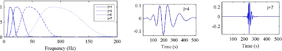
C k . (10)Nevertheless, the excellent time-localization capabilities of Daubechies wavelets, comes at the cost of relatively poor frequency domain localization. This issue is illustrated in Fig.2 (left panel) which plots the magnitude Fourier spectrum,
ˆ ( / 2 ) j
, of Daubechies wavelets “D20” (defined using an N=20-long FIR filter derived and reported in [9]) for four
bank of Fig.1. These plots have been obtained by first constructing the D20 wavelets in the time domain at different scales given the FIR filter coefficients (see also Fig. 2 central and right panels). This is achieved by means of a standard recursive algorithm which constructs recursively the so-called “scaling function”, φ(t), (a fundamental concept of the wavelet theory and multi-resolution analysis [9]) and then the associated wavelet function at each considered scale j by relying on the following “two-scale equations” (see [10] for a numerical implementation)
1 1
(2 )j [ ] (2j )
n
φ t
g n φ t n ,(11)
1 1
(2 )j [ ] (2j )
n
ψ t
h n φ t n .(12)
In (11), the sequence g1[n], n=1,2,…,20 are the coefficients of the FIR filter defining the D20 wavelets. Further, in (12), h1[n]=(-1)
n
[image:6.595.66.554.284.373.2]g1[1-n]. Note that the signal analysis FIR filters appearing on Fig.1 for the D20 wavelets are defined as (quadrature mirror construction) g[n]= g1[n]/2, and h[n]= (-1)n g1[n+1].
Figure 2. Daubechies wavelets “D20”: Normalized to the peak value Fourier magnitude spectrum ˆ ( / 2 ) j
for 4 different scales j (left panel); time
history at scale j=4 (central panel); ); time history at scale j=7 (right panel).
Daubechies DWT filter banks (similar to the one shown in Fig.1) have been utilized to process acceleration vibration response signals from dynamically excited linear structures for structural damage detection purposes in [5] and [11] by considering certain wavelet-based structural damage detection indices as detailed in the following section.
III. THE WAVELET ENTROPY AS A STRUCTURAL DAMAGE DETECTION INDEX
In general terms, “structural damage” due to dynamically induced loads is manifested by non-linear phenomena (e.g., hysteretic energy dissipation during damaging dynamic excitations) and by permanent changes to the (linear) dynamic properties of a structural system (e.g., natural frequencies and mode shapes of vibration). Taking as the time reference the instant at which damage occurs, one can identify three different phases of the structure. The first pre-damage phase corresponds to a “healthy” structural state in which a vibrating structure behaves linearly. The second phase corresponds to the relatively short time interval during which damage takes place. In this phase the structure is characterized by a time-varying non-linear behavior. In the third post–damage phase the structure has already undergone permanent changes; the damage has now been “registered” and the structure behaves linearly under dynamic excitations. In this context, the Shannon wavelet entropy (SWE), originally introduced and considered for biomedical signal processing applications [6] has proved to be a useful tool for detecting, characterizing, and quantifying structural damage by wavelet processing of vibration structural response signals at the post-damage phase and at the pre-damage phase ([5],[11]).
Specifically, the SWE is defined as (e.g. [6],[12])
ln( )
j j
j
SWE
p p , (13)where the summation involves all scales considered in an energy preserving wavelet transformed signal as detailed in the previous section, and pj is the wavelet energy at scale j in (9) relative to the total energy carried by the signal E, that is,
j j
E p
E
. (14)
carried by the signal at different scales and corresponding frequency bands. For example, a signal carrying most of its energy around a specific frequency ω0 (e.g. a realization of a narrow-band stochastic process such as the response of a white-noise excited single-degree-of-freedom oscillator with natural frequency ω0), will have very few relative wavelet energy ratios of significant value: those corresponding to scales whose bandwidth contain ω0 (see also Fig. 2). Consequently, the SWE will take on a negligible value. On the antipode, all relative wavelet energy of a broad-band signal will take on significant values and, therefore, the SWE will also attain a large value.
In this regard, assuming that vibration response signals of the healthy structure at pre-damage phase are available, Ren et al. [5] considered the use of the relative wavelet entropy defined by
ln j
j
j j
p
RWE p
q
, (15)as a structural damage sensitive index. In the last equation, pj the relative wavelet energy at scale j of a vibration (acceleration) signal taken from the “damaged” structure and qj is the relative wavelet energy at scale j of a vibration signal obtained from the “healthy” structure. For structures with negligible damage it is expected that pj≈ qj for all considered j scales and thus RWE attains a negligible value. For damaged structures, it is expected that the two ratios will differ across most of the scales yielding a large RWE value.
Note that the RWE index in (20) is independent of time and thus it is suitable for detecting time-invariant structural damage from post-damage phase ([5],[11]). Since the underlying information for the detection of such kind of damage is associated with signal energy distribution along the frequency domain, it is intuitive to expect that the RWE is strongly dependent on the frequency localization attributes of the wavelet family (or of the corresponding filter bank). To this end, although ideally each level (or “building block”) of dyadic DWT filter bank splits the frequency domain in two half-bands (a low frequency and a high-frequency one), this is not the case in considering Daubechies wavelets as evidenced in Fig.2 (see also [17]). In this respect, in the next section, a discussion on the frequency localization attributes of typical Daubechies DWT fitler bank is included which motivates the consideration of two other wavelet families for structural damage detection purposes by means of the RWE damage index.
IV. ON FREQUENCY SELECTIVITY AND CONSTANT-Q ANALYSIS OF DAUBECHIES DWT FILTER BANKS
By examining the left panel of Fig.2, it is readily noticed that significant overlapping of the wavelet Fourier spectra (or equivalently of the combined frequency response functions of the analysis filter bank) occurs, not only between neighboring scales but even non-adjacent scales. This rather poor “frequency selectivity” between scales j is typical of Daubechies wavelet DWT filter banks (see also [17]) and becomes more severe at lower frequencies. It comes as a trade-off of the excellent time localization properties of Daubechies wavelets. This is a consequence of the well-known “uncertainty principle” which hold for any Fourier pair: enhancing the energy localization of a function in the time-domain deteriorates its frequency resolution and vice versa (see [8] for further details on this issue). In fact, being compactly supported in the time-domain, Daubechies wavelets are infinitely supported in the frequency domain: the Fourier spectra of Daubechies wavelets have small, but non-negligible, periodic “sidelobs” at higher frequencies from the “effective bandwidth” of the main lobe plotted shown in the left panel of Fig.2. Consequently, in practical applications, the signal energy retrieved at each scale in (9), Ej, cannot be uniquely assigned to any particular frequency band. Therefore, it is natural to expect that the incorporation of Daubechies wavelets to compute the RWE in (15) for damage detection purposes, even if it has been extensively considered in the relevant litereature ([5], [11]), it may not be the best possible choice to yield a robust structural damage index. In the following sections two other orthogonal signal energy preserving wavelet families achieving better frequency resolution than Daubechies wavelets are briefly presented and their effectiveness for damage detection based on the RWE is assessed numerically.
In many signal analysis applications a constant-Q analysis is favorable. This is because high-frequency components in time-series are usually well-localized in time, while low-frequency trends are well-spread in time. Nevertheless, this is not necessarily true in processing acceleration response signals from dynamically excited linear structures whose location of the dominant components on the frequency domain depends on the structural natural frequencies. In this regard, the use of non-constant Q wavelet analysis filter banks is a reasonable consideration in order to target natural frequencies related to higher modes of vibration effectively and, consequently, to render the RWE damage index in (15) more sensitive to changes in higher frequencies. The wavelet family presented in section VI can readily achieve custom-made non-constant Q wavelet analysis. It is further noted in passing that the wavelet packet transform (WPT) used in conjunction with typical wavelet families can be considered to “zoom in” pre-specified frequency bands of interest (see e.g. [10]). The WPT considers a wavelet tree decomposition filter bank in which the high-pass and low-pass filters g[n] and h[n] of Figure 1 are applied to both output channels (coefficients) of each previous analysis step and has been applied for vibration-based structural damage detection purposes (e.g. [3],[4]). However, finding the optimum wavelet tree decomposition is a non-trivial and case-specific task, while it does not resolve the issue of frequency selectivity: it only makes it worse (e.g. [10]).
V. MEYER WAVELETS COMPACTLY SUPPORTED IN THE FREQUENCY DOMAIN
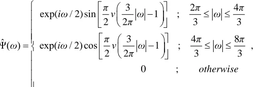
Unlike Daubechies wavelets which are compactly supported in the time domain, the Meyer (mother) wavelet, defined in the frequency domain as (e.g. [9])
3 2 4
exp( / 2) sin 1 ;
2 2 3 3
3 4 8
ˆΨ( ) exp( / 2) cos 1 ;
2 2 3 3
0 ;
π π π
iω v ω ω
π
π π π
ω iω v ω ω
π
otherwise
, (16)
is compactly supported in the frequency domain.In the last equation, the auxiliary function v(u) controls the “smoothness” of the Fourier magnitude spectrum of Meyer wavelets and, therefore, their rate of decay in the domain (i.e., their time-localization attribute). A common smoothing function of choice is (e.g. [9],[18])
4 2 3
(35 84 70 20 ) ; 0,1
( )
0 ;
u u u u u
v u
otherwise
, (17)
[image:8.595.166.425.324.410.2]Orthogonal Meyer wavelet basis functions can be readily constructed and be used within the CWT framework in (5) to achieve energy preserving signal analysis. Further, DWT filter banks comprising FIR filters (as in Fig. 1) approximating Meyer wavelets in an octave frequency domain discretization exist [18],[19]. Such a filter bank is used in the numerical applications of section VII. In fact, Fig. 3 plots Meyer wavelets at the same scales (DWT discretization scheme) as the ones considered in Figs. 1 and 2 for D20 Daubechies wavelets. It is noted, however, that these plots have been obtained directly from (16) and its inverse Fourier transform by considering appropriate scaling factors.
Figure 3. Meyer wavelets- dyadic filter bank: Normalized to the peak value Fourier magnitude spectrum ˆ ( / 2 ) j for 4 different scales j (left panel); time
history at scale j=4 (central panel); ); time history at scale j=7 (right panel).
VI. NON CONSTANT-QWAVELET ANALYSIS VIA THE HARMONIC WAVELET TRANSFORM (HWT)
Introduced by Newland [16], the harmonic wavelet transform (HWT) has been proved a potent tool for structural damage detection of yielding multi-storey building structures under severe earthquake excitation [13]. The HWT incorporates a basis of complex-valued analyzing “harmonic wavelet” functions with compactly supported box-like Fourier spectra. A “general” harmonic wavelet at scale j centered at the k/(p[j]-m[j]) position in time can be written in the frequency domain as (see also [20])
,
2 2 2
exp ;
ˆ
0 ;
o
j k o o o
i kT
m j p j
T T
p j m j T p j m j
otherwise
, (18)
where Το is the total length (duration) of the time interval considered in the analysis. In the last equation, the vectors p and m contain integer positive numbers. It has been shown [16], that a collection of harmonic wavelets spanning adjacent non-overlapping intervals at different scales along the frequency axis forms a complete orthogonal basis (see also [20]). This can be achieved by proper definition of the p and m vectors. Then, the HWT computed by substituting the inverse Fourier transform of (18) in (8), produces coefficients Cj[k] which preserve the input signal energy E. It is noted in passing that the
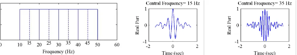
[image:9.595.73.551.443.532.2]Importantly, note that at scale j the effective bandwidth of the HWT is (p[j]-m[j])2π/Το and the central frequency is (p[j]+m[j])π/Το. In this respect, it can be readily seen that HWT enables arbitrary frequency resolution within any given range of frequencies. Furthermore, the effective frequency band at each scale is defined directly in the frequency domain in a straightforward manner. Therefore, the HWT provides for exceptional freedom in defining “frequency bins” of arbitrary width which (theoretically, since “ideal” band-pass filters cannot be numerically implemented using FIR filters) do not overlap. This is not the case for typical wavelet families (e.g., Meyer and Daubechies families) whose frequency content at each scale is implicitly defined by means of a single scalar: the scaling parameter a in (4). An example of four neighboring scales as part of a basis with constant-width “frequency bins” is shown in the left panel of Fig. 4 where the central frequency of each scale is noted by a broken line. Such a basis leads to a non-constant Q analysis as defined in section IV and this can be readily appreciated by comparing Fig. 4 with Figs. 2 and 3. A constant Q analysis with octave (dyadic) frequency domain discretization of the typical DWT can be accommodated by the HWT by taking m[j]=2j and p[j]= 2j+1.
Figure 4. Harmonic wavelets- constant bandwidth filterbank: positive Fourier magnitude spectrum for 4 different scales with central frequencies denoted by broken lines (left panel); real part time history for central frequency 15Hz (central panel); ); real part time history for central frequency 35Hz (right panel).
Nevertheless, the aforementioned “freedom of choice” of HWT comes at the cost of very poor time localization as seen by comparing the wavelet time-histories at different scales plotted in Figs. 2 to 4. In fact, harmonic wavelets can be viewed as the complex counterpart of the so-called “Shannon wavelets” associated with the Littlewood-Paley basis (see for example [9] and [17]), which are well-known for their poor time localization properties. Still, for non-evolutionary damage detection relying on post-damage linear vibration responses, as discussed in section IV, poor time-localization attributes is of secondary importance.
From a computational viewpoint, robust fast Fourier transform (FFT)-based algorithms have been proposed by Newland[16],[21] for the efficient computation of non-redundant as well as for redundant HWT on the frequency domain. A custom-made implementation of Newland’s FFT-based algorithm is used in the numerical part of this work to compute the HWT for non-constant Q harmonic wavelet bases as detailed in the following section.
VII. ASSESSMENT OF DIFFERENT WAVELET FAMILIES FOR WAVELET ENTROPY-BASED DAMAGE DETECTION
A. Methodology
detection algorithms (e.g. [2],[5]]), namely a simply supported linear free vibrating beam excited by an impulse/hammer along the gravitational direction for “healthy”/intact and “damaged” conditions, are considered.
[image:10.595.146.471.343.454.2]In particular, a 5m long steel IPE300-profiled beam with mass density of 7849 kg/m3, elastic modulus of 210 GPa, cross section area of 53.8 cm2 and moment of inertia corresponding to in-plane bending of 8360 cm4 is modelled using 4-node shell elements with 6 degrees-of-freedom per node using a standard commercial finite element (FE) software [22]. The adopted FE mesh is shown in Fig. 5 for the healthy/intact beam (state D0) and for three (post-) damage states, D1, D2, and D3. In the latter states, damage is represented by 50% reduction of the cross sectional area of the intact beam at mid-span (D1), at mid-span and first quarter-span (D2), and at every quarter-span (D3). Table I reports the natural frequencies corresponding to the vertical in-plane first two modes of vibration of the considered FE models obtained by means of standard modal analysis. Further, linear response history analysis is conducted for all 4 FE models of Fig. 5 considering an external point force along the gravity axis applied to the middle of the upper flange at mid-span. The force traces a half-sine time history of 0.01s duration to “simulate” a hammer/impulsive load (see e.g. [23]). A damping ratio of 1% for all modes is assumed in the analysis lasting for 4s with 0.001s time-step. The vertical response acceleration traces at 15 equidistant sensor or “measurement points” located on the upper flange of the beam models (points 1 to15 shown in Fig. 5) are recorded and stored. These output signals are normalized by the energy of the excitation force considered. Further, the first second of these signals is discarded to eliminate the signature of the input force as well as other transient effects [11]. Finally, a total duration of 0.51s from each signal (512 samples sampled at 1000Hz) is kept for further processing corresponding to the strong motion part of the (amplitude-decaying) free vibration acceleration response of the 4 FE models at the 15 measurement points. The consideration of more than one measurement point aims for damage localization apart from damage detection as established in [5] and [11].
[image:10.595.203.415.510.597.2]Figure 5. Cross sectional dimensions and damage locations of the considered IPE300 steel beam.
TABLE I. NATURAL FREQUENCIES (IN HZ) OF THE FIRST THREE MODES FOR THE HEALTHY AND THE DAMAGEDBEAM IN FIG.5
Mode
Beam States
D0
(Healthy) D1 D2 D3
1 54.88 51.91 49.13 49.27
2 153.07 150.81 105.82 79.52
3 313.48 251.64 222.67 173.67
TABLE II. FREQUENCY DOMAIN PROPERTIES OF THE CONSIDERED DAUBECHIES WAVELET BASIS (CONSTANT Q≈0.5ANALYSIS)
Analysis Level (scale)
Daubechies D20 wavelet analysis
Effective bandwidth (Hz)
Characteristic Frequency (Hz)
1 (j=9) 70.62 – 812.14 342.11
2 (j=8) 45.85 – 412.66 171.05
3 (j=7) 21.48 – 207.66 85.53
4 (j=6) 10.41 – 100.66 42.76
5 (j=5) 5.13 – 51.29 21.38
6 (j=4) 2.55 – 25.45 10.69
7 (j=3) 1.27 – 12.68 5.35
8 (j=2) 0.63 – 6.33 2.67
9 (j=1) 0.32 – 3.16 1.34
TABLE III. FREQUENCY DOMAIN PROPERTIES OF THE CONSIDERED MEYER WAVELET BASIS (CONSTANT Q≈0.68ANALYSIS)
Analysis Level (scale)
Meyer wavelet analysis
Effective bandwidth (Hz)
Central Frequency
(Hz)
1 (j=9) 179.2 – 665.6 331.68
2 (j=8) 89.6 – 332.8 165.84
3 (j=7) 44.8 – 166.4 82.92
4 (j=6) 22.4 – 84.27 41.46
5 (j=5) 11.2 – 41.6 20.73
6 (j=4) 5.6 – 21.07 10.37
7 (j=3) 2.8 – 10.53 5.18
8 (j=2) 1.4 – 5.27 2.59
9 (j=1) 0.70 – 2.67 1.30
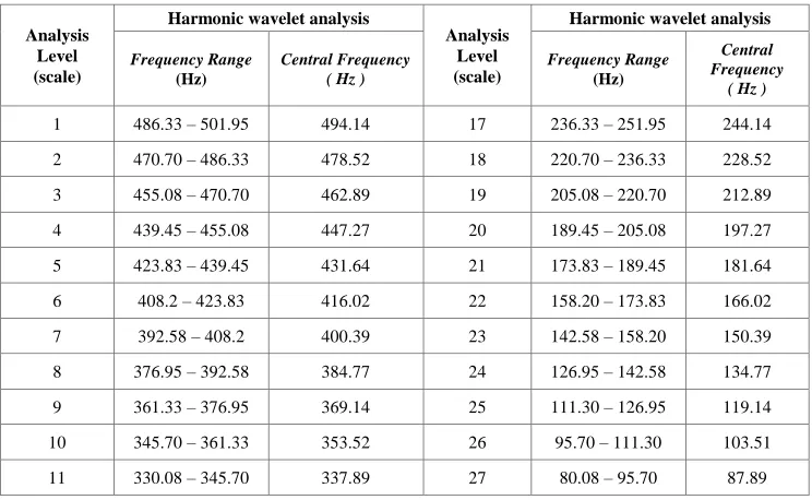
TABLE IV. FREQUENCY DOMAIN PROPERTIES OF THE CONSIDERED HARMONIC WAVELET BASIS (NON-CONSTANT QANALYSIS)
Analysis Level (scale)
Harmonic wavelet analysis
Analysis Level (scale)
Harmonic wavelet analysis
Frequency Range
(Hz)
Central Frequency ( Hz )
Frequency Range
(Hz)
Central Frequency
( Hz )
1 486.33 – 501.95 494.14 17 236.33 – 251.95 244.14
2 470.70 – 486.33 478.52 18 220.70 – 236.33 228.52
3 455.08 – 470.70 462.89 19 205.08 – 220.70 212.89
4 439.45 – 455.08 447.27 20 189.45 – 205.08 197.27
5 423.83 – 439.45 431.64 21 173.83 – 189.45 181.64
6 408.2 – 423.83 416.02 22 158.20 – 173.83 166.02
7 392.58 – 408.2 400.39 23 142.58 – 158.20 150.39
8 376.95 – 392.58 384.77 24 126.95 – 142.58 134.77
9 361.33 – 376.95 369.14 25 111.30 – 126.95 119.14
10 345.70 – 361.33 353.52 26 95.70 – 111.30 103.51
Analysis Level (scale)
Harmonic wavelet analysis
Analysis Level (scale)
Harmonic wavelet analysis
Frequency Range
(Hz)
Central Frequency ( Hz )
Frequency Range
(Hz)
Central Frequency
( Hz )
12 314.45 – 330.08 322.27 28 64.45 – 80.08 72.27
13 298.83 – 314.45 306.64 29 48.83 – 64.45 56.64
14 283.20 – 298.83 291.02 30 33.20 – 48.83 41.06
15 267.58 – 283.20 275.39 31 17.58 – 33.20 25.39
16 251.95 – 267.58 259.77 32 1.95 – 17.58 9.77
Next, the relative wavelet energy at each scale of the three different wavelet bases of tables II to IV is computed from the wavelet coefficients of the total 60 simulated linear response acceleration signals (15 signals from four FE models of Fig.5), using (9), (10), and (14). Finally, the following “scale-dependent” contributor to the overall relative wavelet entropy in (15) is calculated for all 15 measurement points of the three damaged states
jln jj p
RWE j p
q
. (19)
In the last equation, qj is the relative wavelet energy at scale j computed from the simulated response signals of the D0 “healthy” beam, while pj is the relative wavelet energy at scale j corresponding to response signals of the damaged states. The above “scale-dependent” RWE makes possible to discriminate the contributions to the overall RWE in (15) from each wavelet analysis scale. Therefore, it serves well the purpose of assessing the influence of the frequency domain attributes of the three different wavelet families considered (i.e., frequency selectivity between scales and Q-factor) to their potential for damage detection and localization via the RWE index. The next subsection presents and discusses the results of the analyses undertaken in terms of scale-dependent RWE(j).
B. Numerical results and discussion
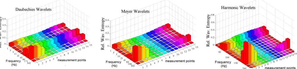
The scale-dependent relative wavelet energy RWE(j) defined in (19) is plotted in three-dimensional bar plots in Figs. 6,7, and 8 for the damage states D1, D2, D3, respectively, as obtained from the Daubechies wavelet basis of table II (left panel of Figs. 6 to 8), the Meyer wavelet basis of table III (central panel of Figs. 6 to 8), and the harmonic wavelet basis of table IV (right panel of Figs. 6 to 8). The RWE(j) bars are stacked along a “frequency axis” labeled after the “characteristic” or “central” corresponding to each scale j and along a “spatial axis” corresponding to the 15 equidistant measurement points considered along the length of the vibrating beam.
Non-zero RWE(j) values at a particular scale suggests changes to the energy content carried at the frequency band corresponding to this scale which is indicative of a “damage” compared to the healthy (reference) structure. Theoretically, such changes (or peak RWE(j) values) are expected at scales (sub-bands) containing the natural frequencies of the damage state reported in table I. Indeed, in all furnished plots non-zero RWE(j) values are observed at around scales with characteristic frequency of about 50Hz which corresponds roughly to the natural frequency of the first vertical in-plane mode shape of all three damaged beams. Thus, in all cases, the RWE is able to “detect” damage, despite the remarkable differences in the distribution of RWE(j) for each damage state due to the use of different wavelet bases. More importantly, the herein adopted scale-dependent RWE(j) contributor needs to be interpreted by bearing in mind the spatial correlation of the vertical modes of vibration. For example, the D1 damage state cannot be detected by the RWE(j) for scales close to the natural frequency of the second vertical mode of vibration. This is because the damage in D1 is located at a “stationary” point of the second mode shape. Further, the damage at the first quarter of the beam in D2 state is better detected by the RWE(j) values close to the second natural frequency of the damaged beam at approximately 105Hz, rather than the first
100Hz at measuring points 1 to 5) and the damage at midspan revealed by the RWE(j) value at 50Hz. Similar remarks hold for the D3 case. The non-constant Q harmonic wavelet analysis is able to distinguish and localize the three damages along the frequency (at 50Hz and at 170Hz corresponding to the first and to the third natural modes of the D3 beam) and the spatial axes (at the first and last quarters of the beam and at midspan), better than the Daubechies and the Meyer wavelet bases.
[image:13.595.62.566.314.427.2]Figure 6. Scale-dependent relative wavelet entropy (RWE(j) in (19)) derived using different wavelet families for damage state D1 of Fig.5.
Figure 7. Scale-dependent relative wavelet entropy (RWE(j) in (19)) derived using different wavelet families for damage state D2 of Fig.5.
Figure 8. Scale-dependent relative wavelet entropy (RWE(j) in (19)) derived using different wavelet families for damage state D3 of Fig.5.
VIII. CONCLUDING REMARKS
[image:13.595.59.558.457.573.2]have a theoretically infinite support in the frequency domain and, therefore, the Daubechies DWT filter bank has a relatively poor level of frequency selectivity among scales.
Nevertheless, it is important to emphasize that this paper is limited to the case of “stationary” (time-invariant) damage. In cases of monitoring the dynamic response of structures “as they are being damaged” (e.g., during strong earthquake excitations), or in cases it is desired to locate the time instant at which damage occurs (e.g., real-time monitoring of structures), the use of well-localized in time wavelet analysis functions, such as Daubechies wavelets, should be more effective for damage identification purposes via a time-dependent RWE.
Furthermore, one should not draw the erroneous conclusion that Daubechies, Meyer, and other standard wavelet families are not capable for better frequency localization in the context of the DWT. The concept of wavelet packet transform (WPT) which generalizes the DWT to process the detailed (wavelet) coefficients at each scale can be employed to zoom in the frequency domain at will. In fact, the harmonic wavelet transform can be also interpreted as a WPT kind of analysis since it allows to subdivide each spectral box into an arbitrarily large number of boxes of reduced bandwidth. However, the use of WPT has not been pursued in this work. Accordingly, harmonic wavelet bases of uniform bandwidth at each scale have been considered such that no “zooming in” at any particular frequency is considered. Moreover, other standard techniques used in practical signal processing applications to achieve finer frequency domain discretization, such as the artificial increase of the length of the acceleration signals by means of zero-padding, have also been left out of this work. In any case, the herein furnished numerical results point to the fact that frequency selectivity and localization/discrimination is a desirable attribute to enhance the ability of the RWE for stationary damage identification, though “targeting” specific frequencies implies that natural frequencies of the damaged state are known a priori. The latter may not be readily available in practical structural health monitoring (SHM) scenarios.
Overall, it can be concluded that the choice of the type of wavelets to be adopted in RWE-based damage detection is an important issue that affects the performance of this particular damage index. Further research is warranted towards providing practical recommendations on fine-tuning or optimizing the time and frequency domain properties of the analyzing wavelet basis according to particular SHM application; this consideration seems to have been overlooked in the literature and it is recommended that future research work should be devoted on this aspect.
REFERENCES
[1] K. Worden, C.R. Farrar, G. Manson and G. Park, “The fundamental axioms for structural health monitoring,” Proceedings of the Royal Society,
London A, Vol. 463, pp. 1639-1664, 2007.
[2] J. Humar, A. Bagchi and H. Xu, “Performance of vibration-based techniques for the identification of structural damage,” Structural Health Monitoring, Vol. 5(3), pp.215-227, 2006.
[3] G.G. Yen and K.-C. Lin, “Wavelet packet feature extraction for vibration monitoring,” IEEE Transactions on Industrial Electronics, Vol.47, pp. 650-667, 2000.
[4] Z.Sun and C.C. Chang, “Statistical wavelet-based method for structural health monitoring,” Journal of Structural Engineering, Vol. 130, pp. 1055-1062, 2004.
[5] W.-X. Ren and Z.-S., Sun, “Structural damage identification by using wavelet entropy,” Engineering Structures, Vol. 30, no.10, pp. 2840-2849, 2008. [6] S. Blanco, F. Figliola, R. Quian Quiroga, O.A. Rosso and E. Serrano, “Time–frequency analysis of electroencephalogram series (III): information
transfer function and wavelets packets,” Physical Review E, Vol.57, pp.932-940, 1998.
[7] Shannon CE. A mathematical theory of communication: I and II. Bell System Tech J 1948;27:379–443. [8] L. Cohen L, Time- Frequency Analysis. New Jersey: Prentice-Hall, 1995.
[9] I. Daubechies, Ten Lectures on Wavelets. Philadelphia: SIAM, 1992.
[10] J.C. Goswami and A.K. Chan, Fundamentals of wavelets: Theory, algorithms, and applications. New York: Wiley, 1999.
[11] G.J. Yun, S.-G. Lee, J. Carletta and T. Nagayama, “Decentralized damage identification using wavelet signal analysis embedded on wireless smart sensors”, Engineering Structures, Vol. 33, no. 7, pp. 2162-2172, 2011.
[12] O.A. Rosso, M.T. Martin, A. Figliola, K. Keller and A. Plastino, “EEG analysis using wavelet-based information tools,” Journal of Neuroscience Methods, Vol. 153, pp. 163-182, 2006.
[13] P.D. Spanos, A. Giaralis, N.P. Politis and J.M. Roessett, “Numerical treatment of seismic accelerograms and of inelastic seismic structural responses using harmonic wavelets,” Computer-Aided Civil and Infrastructure Engineering, Vol.22, pp. 254-264, 2007.
[14] P.D. Spanos, A. Giaralis, N.P. Politis, “Time- frequency representation of earthquake accelerograms and inelastic structural response records using the adaptive chirplet decomposition and empirical mode decomposition,” Soil Dynamics and Earthquake Engineering, Vol.27, pp. 675-689, 2007. [15] J. C. Brown, “Calculation of a constant Q spectral transform,” Journal of the Acoustical Society of America, vol. 89, no.1, pp.425–434, Jan.1991. [16] D. E. Newland, “Harmonic and musical wavelets,” Proceedings of the Royal Society, London A, Vol. 444, pp. 605-620, 1994.
[17] M. Vetterli and C. Herley, “Wavelets and filter banks: theory and design,” IEEE Transactions of Signal Processing, Vol. 40(9), pp. 2207-2232,1992. [18] M. Misiti, Y. Misiti, G. Oppenheim, J. Poggi, Wavelet Toolbox, The MathWorks Inc, 2000.
[19] P. Abry, Ondelettes et turbulence. Multiresolutions, algorithms de decomposition, invariance d’ echelles. Paris: Diderot Editeur, 1997.
[20] A. Giaralis and P.D. Spanos, “Wavelet-based response spectrum compatible synthesis of accelerograms-Eurocode application (EC8),” Soil Dynamics Earthquake Engineeing, Vol. 29, pp. 219-235, 2009.
[21] D.E. Newland, “Ridge and phase identification in the frequency analysis of transient signals by harmonic wavelets,” Journal of Vibrations and Acoustics, Vol.121, pp. 149-155, 1999.
[22] CSI Analysis Reference Manual, for SAP2000, ETABS and SAFE. Computers and Structures Inc, 2007.
![Figure 1. Typical dyadic discrete wavelet transform (DWT) analysis filter bank with J=9 scales for processing of N=512 long discrete-time signals x[n]](https://thumb-us.123doks.com/thumbv2/123dok_us/1508814.103557/5.595.62.556.379.494/figure-typical-discrete-wavelet-transform-analysis-processing-discrete.webp)