1
Effective and efficient midlevel visual elements-
oriented land-use classification using VHR remote
sensing images
Gong Cheng1, Junwei Han1, Lei Guo1, Zhenbao Liu2, Shuhui Bu2, Jinchang Ren3 1
School of Automation, Northwestern Polytechnical University, Xi’an, 710072, China 2
School of Aeronautics, Northwestern Polytechnical University, Xi’an, 710072, China 3
Department of Electronic and Electrical Engineering, University of Strathclyde, UK
Abstract
Land-use classification using remote sensing images covers a wide range of applications. With more detailed spatial and textural information provided in very high resolution (VHR) remote sensing images, a greater range of objects and spatial patterns can be observed than ever before. This offers us a new opportunity for advancing the performance of land-use classification. In this paper, we first introduce an effective midlevel visual
elements-oriented land-use classification method based on “partlets,” which are a library of pretrained part detectors used for midlevel visual elements discovery. Taking advantage of midlevel visual elements rather than low-level image features, a partlets-based method represents images by computing their responses to a large number of part detectors. As the number of part detectors grows, a main obstacle to the broader application of this method is its computational cost. To address this problem, we next propose a novel framework to train
coarse-to-fine shared intermediate representations, which are termed “sparselets,” from a large number of
pretrained part detectors. This is achieved by building a single-hidden-layer autoencoder and a single-hidden-layer neural network with an L0-norm sparsity constraint, respectively. Comprehensive evaluations on a publicly available 21-class VHR land-use data set and comparisons with state-of-the-art approaches demonstrate the effectiveness and superiority of this paper.
Keywords:
Autoencoder, land-use classification, midlevel visual elements, part detectors, remote sensing images.1.
Introduction
Land-use classification plays an important role for a wide range of applications, such as natural geological hazards detection [1, 2], general land-use/land-cover (LULC) determination[3-17],
2
vegetation types mapping [18], environment monitoring, and urban planning, etc. Although significant efforts have been made in developing various approaches to infer land usage from satellite and aerial images during the last decades, how to effectively understand the meaning and contents of images remains one of the most challenging problems in the field of remote sensing images analysis.
Most previous works [8-17] mainly focus on classifying pixels or objects (or rather, grouping of local homogeneous pixels) into their thematic class by extracting low-level image features (e.g. texture feature [9, 10], color feature [8], spatial and spectral information [11-13], or their hybrids [14-17]) as classification features. For example, Bhagavathy and Manjunath [9] used textures features to model and classify compound objects with spatially recurrent patterns, such as harbors and golf courses. Li et al. [8] presented a new land cover classification method by adopting an improved color structure code for segmentation and support vector machine (SVM) using high resolution QuickBird data. Chen et al. [13] proposed a novel nonlinear technique for hyperspectral image classification by representing each pixel via kernel sparse representation in spatial and spectral feature space. Zhang et al. [17] introduced a framework to linearly combine multiple features in a optimal way to obtain a unified low-dimensional representation of multiple features for hyperspectral remote sensing image classification.
3
classification using very high resolution (VHR) remote sensing images has attracted more and more attentions [3-7, 19, 20] because of its foundation and importance in automated image content understanding.
A kind of widely used approaches for scene-level land-use classification are bag-of-visual-words (BOVW) model [21] and its variations [2, 5-7]. The BOVW model treats each image as a collection of unordered local features (e.g. scale invariant feature transform (SIFT) [22] descriptor), quantize them into a limited set of visual words, and then compute a compact histogram representation for scene classification, which is robust against spatial variations but disregards the spatial layout of the features. Combining spatial information with BOVW model, Yang and Newsam proposed spatial co-occurrence kernel (SCK) [6] and spatial pyramid co-occurrence kernel (SPCK) [7] by considering the relative spatial arrangement of the visual words and both of the absolute and relative spatial layout of an image, respectively. Zhao [5] further extended the traditional BOVW model to a 2-D wavelet decomposition (WD)-based BOVW model for 21 classes LULC scene classification. The WD-based BOVW method considered both spatial arrangement and textural information by constructing several different visual dictionaries from original images and their corresponding 2-D wavelet decomposition sub-images.
4
joint sparse coding (MFJSC) with spatial relation constraint.
These previous methods have been proven to be effective for VHR image land-use classification tasks, but as the land-use scene classification task becomes more challenging, the semantic gap between low-level feature representations and the meaning of images increases, so they are still difficult to obtain better performance without addressing this problem. Take eight VHR images with 0.3 m pixel resolution of Fig. 1 as examples, which are from a publicly available 21 LULC classes data set1 [6, 7]. An image classification method based on low-level image features, such as texture, spectral, or color histogram, would easily misclassify images (a) and (b), (c) and (d), (e) and (f), and (g) and (h) as the same LULC class. Even by introducing some spatial layout information of the whole image would do little to differentiate them accurately. However, humans would classify them as belonging to different LULC classes based on discriminative objects (e.g. putting green, water, cars, runway marking, grass line, tennis court, and buildings, etc.) and the high-level semantic concepts pertaining to the classes. This example and our visual experiences suggest that a straightforward and effective way to classify challenging image scenes would be discriminative object-oriented method.
5
Fig. 1. Eight VHR images from LULC class (a) baseball diamond, (b) tennis court, (c) freeway, (d) runway, (e) golf course, (f) river, (g) tennis court, (h) and sparse residential.
The VHR remote sensing images have been providing us more and more detailed spatial and textural information, in which a greater range of objects and spatial patterns can be observed than ever before because of the increased sub-meter resolution. With the fine resolution, individual objects, such as cars, trees, and buildings, etc., are now recognizable and can be separately identified. This provides us new opportunity to train more and more object detectors and further advance the performance of scene-level land-use classification by adopting object-oriented image representation scheme.
Guided by this observation and motivated by the idea of using object detectors as the basic representation of images, in this paper, we first introduce an effective scene-level land-use classification method using a library of pre-trained object detectors which are called ‘objectlets’ hereinafter. In the introduced land-use classification scheme, we use discriminative objects rather than individual pixels as attributes to represent images by computing their responses to a large number of pre-trained object detectors. This image representation method provides a solution for narrowing the semantic gap between low-level image features and high-level meaning and contents of the image, making it more suitable for complex real-word land-use classification task.
6
thought of as a generic part that is shared between all object classes. With this representation, the part responses of a DPM, for any object class, can be approximately reconstructed as sparse combinations of the sparselets with their corresponding activation vectors. However, the method proposed by Song et al. [23] for learning sparselets and activation vectors is obviously brittle, in which sparselets and activation vectors were approximately obtained by using greedy algorithms such as orthogonal matching pursuit algorithm (OMP) [25-27] without fully exploiting the discriminative information hidden in training samples. Although these sparse coding based sparselets led to a great computational savings, they also resulted in a substantial loss in detection accuracy.
Based on our introduced objectlets, in this paper, we next propose and formulate a new and extremely effective framework to train coarse-to-fine sparselets for efficient object-oriented land-use classification. Specifically, we first train coarse sparselets using an unsupervised single-hidden-layer auto-encoder [28-31], while applying careful cross-validation to prevent over-fitting. Then, we simultaneously train fine sparselets and activation vectors using a supervised single-hidden-layer neural network. In order to adequately explore the discriminative information hidden in the training samples and to make the learned activation vectors to be sparse, we propose to optimize a new discriminative objective function by imposing L0-norm sparsity constraint on the activation vectors. Using the trained sparselets we achieved efficient object-oriented land-use classification with great speedup factors but almost no decrease in task performance.
7
between low-level feature representation and high-level visual recognition tasks. Second and the most important, to save computational costs while preserve a desired accuracy, we propose and formulate a new and extremely effective framework to train shared intermediate representations, i.e., sparselets, from a large number of pre-trained object detectors. This is achieved by training an unsupervised single-hidden-layer auto-encoder and a supervised single-hidden-layer neural network with L0-norm sparsity constraint, respectively. The proposed framework can achieve efficient object-oriented VHR image land-use classification with great speedup factors but almost no decrease in task performance. Third, comprehensive evaluations on a challenging 21 classes VHR LULC data set and comparisons with state-of-the-art approaches demonstrate the effectiveness and superiority of our work. To the best of our knowledge, this result is the best on this data set.
The rest of the paper is organized as follows. Section 2 introduces objectlets and objectlets-based land-use classification method. Section 3 describes coarse-to-fine sparselets training framework in detail. Section 4 presents comparative experimental results on a publicly available 21 classes VHR land use/land cover data set. Finally, conclusions are drawn in Section 5.
2.
Objectlets
2.1
Objectlets overview
8
trained by taking advantage of the technology of mid-level visual elements discovery [35-37] in a weakly supervised learning scheme where only image category labels are provided. This is particularly important for scene-level VHR image classification, because image-level label can free experts from onerous manual annotation needed by supervised methods.
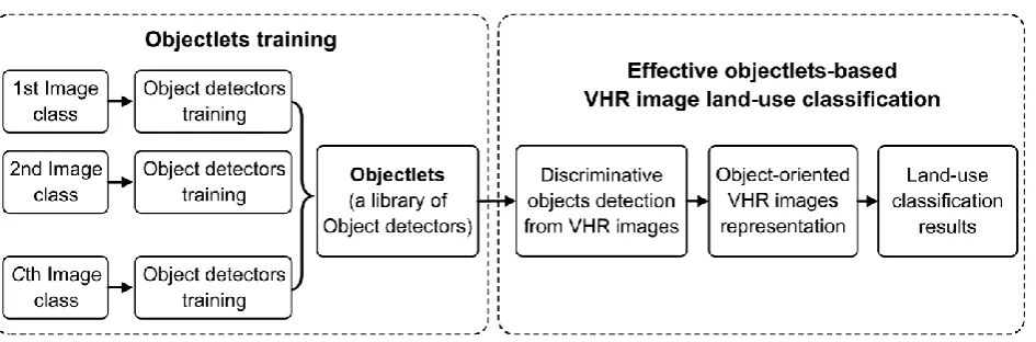
[image:8.595.65.538.517.673.2]Fig. 2 gives an overview of the introduced objectlets-based VHR image land-use classification method. It is mainly composed of two stages: objectlets training and land-use classification. In the objectlets training stage, given an image database, we first train a set of class-specific object detectors for each image class, in histogram of oriented gradients (HOG) [33] feature space, from visual clusters of image patches that have consistent scale, viewpoint, and appearance. This can be easily achieved by sampling a large number of image patches from the positive training images, clustering them, and alternating between training object detectors and refining clusters. Then, all object detectors from all image classes are combined to obtain objectlets. In the land-use classification stage, we first run the trained objectlets to detect discriminative objects from each VHR image, represent the image by computing its response to pre-trained object detectors, and then perform classification by using simple off-the-shelf classifier such as linear SVM classifier.
Fig. 2. Overview of the objectlets-based VHR image land-use classification method.
2.2 Objectlets training
9
(1) (2) ( )
, , C
L denote objectlets for , and ( )
1, 2, , c 1, ,
c
c c cJ c C
L L denote a set
of class-specific object detectors for image class c, where Jc is the total number of object detectors
of ( )c . The training of ( )c for class c
is performed in terms of the following steps [24, 35]:
(1) Construct positive image data set Pc using the images of class c and negative image data set
c
N using the images of the classes ( c).
(2) Sample a large number of image patches from all images in Pc at different scales, discard highly
overlapped patches, perform standard k-means clustering over these patches, in HOG [33] feature space, with the cluster number set to be one tenth of the total number of patches, and then retain clusters with size of ten or more.
(3) Train an object detector cj
wcj,bcj
j1, ,L Jc
for each cluster by optimizing the followingobjective function:
2
* T T
( , )
1
( , ) = arg min ( ) ( )
2
cj cj cj cj
cj cj cj cj cj cj cj
b x X x X
b h x b h x b
ww w w w (1)
where Xcj and
cj
X denote the sets of positive examples and negative examples of j-th cluster,
corresponding to image patches within this cluster and all hard negative examples of Nc, respectively.
( )x
and ( )x denote the HOG feature vectors of positive example x and negative example x. h( ) max 0,1
is standard hinge loss function and is a constant set to 0.1 in our work.(4) Run c on Pc to update clusters from the top-n high-scoring patches for each detector. In our
work we set n10 to keep each cluster being highly pure.
(5) Repeat steps (3) and (4) L iterations to obtain final object detectors ( )c for image class c
.
10
11
[image:11.595.107.491.49.710.2]12 2.3 Objectlets-based land-use classification
The core of objectlets-based land-use classification is to represent images by using discriminative object as attributes, which can be achieved by computing their response to pre-trained objectlets. Specifically, given a VHR image, we first run objectlets on its HOG [33] feature pyramid to compute its response for each location and select the top-M high-scoring detections measured by their responses and their corresponding object detector labels. Then, the responses are normalized to [0, 1] and the image is represented as a feature vector by accumulating all normalized responses to their corresponding object detectors. Finally, we train a linear one-vs-all SVM classifier for each image class by treating the images of the chosen class as positive instances and the rest images as negative instances. An unlabeled test image is assigned to label of the classifier with the highest response.
3.
Sparselets
3.1 Sparselets overview
Sparselets were firstly introduced by Song et al. [23] as a new shared intermediate representation for multi-class object detection for the purpose of accelerating multi-class object detection. In brief, sparselets are a generic dictionary [ , , ,1 2 ]
m K K
D d d d learned from a number of pre-trained object detectors [ ,1 2, , ] [ ,1 2, , ] m N
N N
w w w (to simplify the formulation we omit the
bias term b), where each column m
1, 2, ,
k k K
d is called a spaselet, K is the dictionary
size, and N is the total number of object detectors and N
Cc1Jc in our work. Denoting the HOGfeature pyramid of an image as , the computational bottleneck of object detection is convolution of
with a set of detectors, but in the framework of sparselets, the response for each detector
1, 2, ,
i i N
can be approximated as a sparse linear combination of sparselets D by:
K1
K1
i i k ik k k ik k
13
where denotes the convolution operator and T
1 2
[ , , , ] K
i i i iK
α is an activation vector of
i
with only a few nonzero elements.
For sparselets dictionary size K, total number of detectors N, sparselet dimensionality m, let 0
denote the average number of nonzero elements in T 1 2
[ , , , ] N K
N
α α α α , the speedup factor provided by the sparselets can be written as:
0
Nm Km N
(3)
where Nm and Km N 0 are the approximate operations for each feature pyramid location based on
an exhaustive convolution detection scheme and sparselets model scheme respectively. To make the speedup factor large, the dictionary size K should be much smaller than the total number of detectors
N, and the average number of nonzero coefficients 0 should be much less than the sparselet size m.
Noting that Km is independent of the number of detectors and depends only on the dictionary size which is fixed, as the number of detectors grows, the cost of computing sparselet responses becomes fully amortized which leads to a maximum theoretical speedup of m 0 [23].
14
[image:14.595.59.540.78.251.2]using the same way as objectlets-based land-use classification method.
Fig. 4. Overview of the sparselets-based VHR image land-use classification method.
3.2 Coarse-to-fine sparselets training
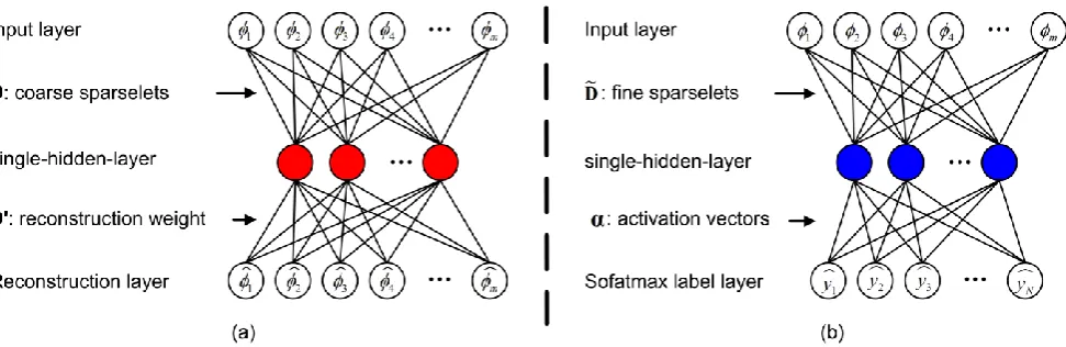
Fig. 5 gives the framework of our presented coarse-to-fine sparselets training: (1) we first train coarse sparselets using an unsupervised single-hidden-layer auto-encoder [28-31], while applying careful cross-validation to prevent over-fitting; (2) we simultaneously train fine sparselets and discriminative activation vectors, using a supervised single-hidden-layer neural network with L0-norm sparsity constraint, to adequately explore the discriminative information hidden in the training samples. Next we will describe the two training processes in detail.
[image:14.595.57.543.503.661.2]15
3.2.1 Coarse sparselets training based on unsupervised auto-encoder
Algorithm 1: Coarse sparselets training based on SA
Input: a library of N pre-trained object detectors [ ,1 2, , ] m N N
and a set of training examples with their HOG features Φ [ (1), (2), ,(Nn)] m Nn
Output: a dictionary of coarse sparselets [ , , ,1 2 ] m K K
D d d d
1: begin
2: Initialize D subjected to ||dk|| 12
3: Initialize reconstruction weight ' [ ,1 2, , ] m K K
D d' d' d'
4: while stopping criterion has not been met do
5: compute the average activation k and Kullback-Leibler divergence KL( k) for each hidden node using (7) and (6)
6: compute reconstruction layer outputs ( )r using (5) 7: compute objective function F1
D D, ';Φ
using (4)8: update D and D' using L-BFGS algorithm, subjected to ||dk|| 12
9: end while 10: return D
11: end begin
The proposed coarse sparselets training is based on a single-hidden-layer auto-encoder (SA), an unsupervised learning architecture used to pre-train neural networks, as shown in Fig. 5(a) and Algorithm 1. In the following sparselets training processes, we will use the same symbols as sparselets description rather than their conventional usages to better understand our method.
Specifically, suppose we have N object detectors [ ,1 2, , ] m N N
and each detector has
n corresponding training examples obtained in subsection 2.2, the input of the auto-encoder is Nn
m-dimensional HOG features of training examples while we use N object detectors for validation to prevent over-fitting. Let Φ [ (1), (2), ,(Nn)] m Nn denote the Nn input data of auto-encoder,
( ) T
1 2
[ , , , ] 1, 2, ,
r m
r r rm r Nn
denote an input of Φ and ( ) T
1 2
[ , , , ]
r m
r r rm
denote the reconstruction of ( )r , our purpose is to learn weights
1 2
[ , , , ] m K
K
D d d d and
1 2
' [ , , , ] m K
K
16
i.e., ( )r ( )r , by minimizing the following objective function
1 , ';
F D D with activation sparsity constraint to hidden layer:
( ) ( ) 21
1 1
1
, '; + KL( )
2 Nn K r r k r k F
Nn
D D (4)
( )
T ( )
' 1 exp r r D D (5) 1
KL( ) log (1 ) log
1 k k k (6)
T ( )
1 11
1 exp
Nn r
k r k
Nn
d (7)where D is the coarse sparselets we attempt to learn subjected to dk 2 1, k 1, 2, ,K, D' is
reconstruction weight which reconstructs the input layer from the hidden layer, K is the number of neurons in the hidden layer corresponding to the sparselets dictionary size, is the weight of the
sparsity penalty, is the target average activation of the hidden nodes, and k is the average activation of the k-th hidden node over the Nn training data. The Kullback-Leibler divergence KL( )
is a standard function for measuring how different two different distributions are, which provides the sparsity constraint. Here we set 3 and =0 05. as suggested in [30].
We can see easily that the objective function given by (4) mainly measures an average reconstruction
17
3.2.2 Fine sparselets and discriminative activation vectors training based on supervised neural
network
Algorithm 2: Fine sparselets and discriminative activation vectors training based on SNN Input: a library of N pre-trained object detectors [ ,1 2, , ]
m N
N
, a set of training examples with their HOG features Φ [ (1), (2), ,(Nn)] m Nn and their labels
(1) (2) ( )
[ , , , Nn ] N Nn
Y y y y
Output: a dictionary of fine sparselets [ , , ,1 2 ] m K K
D d d d , and discriminative activation
vectors T
1 2
[ , , , ] N K
N
α α α α
1: begin
2: Initialize D to be the same as D
3: Initialize activation vectors α using (11) 4: while stopping criterion has not been met do 5: compute the predicted label y( )r using (10) 6: compute regularization term Z
α using (9)7: compute discriminative objective function F2
D, ; ,α y
using (8)8: update D and α using L-BFGS algorithm, subjected to ||dk|| 12 and i 0 0
9: end while 10: return D and α
11: end begin
Notice that we have a large number of training examples with confident labels. In order to incorporate this information to adequately explore the discriminative information hidden in the training examples, we further train fine sparselets [ , , ,1 2 ] m K
K
D d d d and simultaneously learn discriminative activation vectors α by building a supervised single-hidden-layer neural network (SNN) with L0-norm sparsity constraint, as illustrated in Fig. 5(b) and Algorithm 2. Different from reconstruction layer of Fig. 5(a), the output layer is now a binary vector with a softmax unit that allows
one element to be 1 out of N-dimensions for N-way classification problem. The sparselets D are now not only learned from reconstructing the input data, but also a classifier predicting the labels. A discriminative objective function computes an average classification loss between the actual label
( ) T
1 2
[ , , , ] 1, 2, ,
r N
r r rN
y y y r Nn
y = and the predicted label ( ) T
1 2
[ , , , ]
r N
r r rN
y y y
18
More precisely, the discriminative objective function F2
D, ; ,α y
with L0-norm sparsity constraint can be rewritten as:
( ) ( ) 2
2 1 1 , ; , + 2 Nn r r r F Z Nn
D α y y y α (8)
1 20
2 0
1 subject to , 1, 2, ,
2 N
i i
i
Z α
i N (9)
T
( )r softmax αD ( )r
y (10)
where D is the fine sparselets we attempt to learn subjected to
2 1, 1, 2, ,
k k K
d , α is to be
learned discriminative activation vectors,softmax
exp
'exp
1, 2, , ; N
i i i i
a a
a i N a ,1
is a weight decay parameter controls the relative importance of the two terms which was set to be
0.001 as suggested in [30], 0 is the number of nonzero elements in each activation vector.
In the discriminative objective function of (8), the first term represents the supervised goal ensuring that learned sparselets are also going to be good for discriminating between different object detectors. The second term is a regularization term that tends to decrease the magnitude of the activation vectors and helps prevent over-fitting, while with L0-norm sparsity constraint to ensure their sparsity. Similar to coarse sparselets training, we solve this optimization problem by using L-BFGS algorithm [38]. However, noticing the second term is not a convex optimization problem, we adopt an alternative method to approximately minimize it by employing two steps process. To be specific, in the first step, based on the learned coarse sparselets D, we initialize the activation vectors by minimizing the average reconstruction error between all object detectors and their reconstruction approximation via the following formulation:
0 0 1
1
min N i i subject to i , 1, 2, ,
i
i N
N
D . (11)19
[23]. In the second step, the initialization of nonzero variables is fixed, which leads to the satisfaction of the sparsity constraint and results in convex optimization problem to solve. We then learn the selected variables discriminatively according to (8).
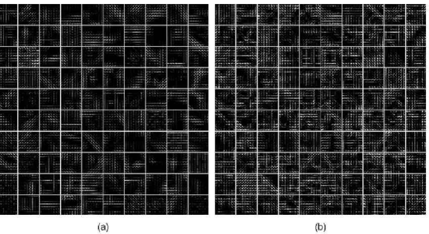
[image:19.595.94.519.300.532.2]In Fig. 6 we show 100 sparselets that we learned from 3093 object detectors trained on the 21 LULC classes data set, using our proposed SNN-based method and sparse coding based method [23], respectively. As can be seen from it, the sparselets learned with our proposed method have more regular structures, such as horizontal, vertical, and diagonal edges, as well as arcs and corners, compared to that learned with sparse coding based method.
Fig. 6. 100 sparselets learned from 3093 object detectors trained on the 21 LULC classes, using (a) our proposed SNN-based method and (b) sparse coding based method [23], respectively.
3.3 Sparselets-based land-use classification
20
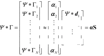
can recover individual object detector response via sparse matrix multiplication with the activation vector replacing the exhaustive convolution operation as shown in (12):
1 1 1 2 2 2 K N N αS d d d (12)
where S is the matrix of all sparselet responses, α is the matrix of sparse activation vectors. Note that the summation is only over non-zero elements of the sparse vector i, which could be efficiently
implemented as sparse matrix multiplications or lookups. Finally, images are represented and classified by using the same way as objectlets-based image classification method.
4.
Experiments
4.1 LULC data set description
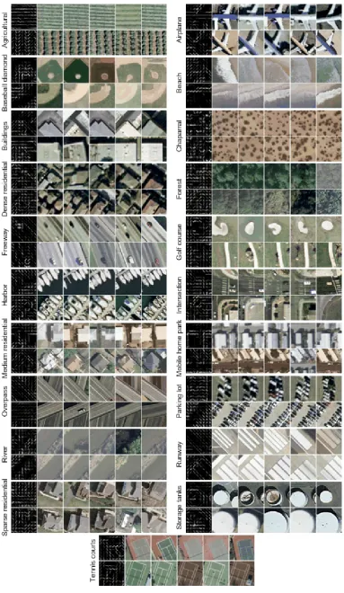
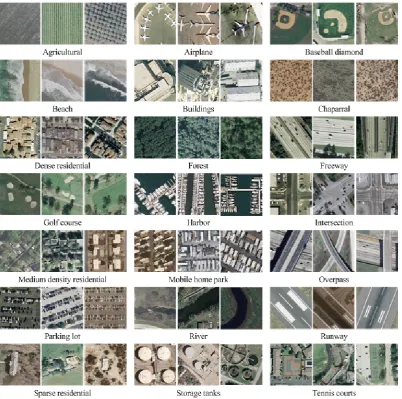
[image:20.595.195.400.120.231.2]21
Fig. 7. Some example images from the 21-class LULC data set.
4.2 Experimental setting
When detecting discriminative objects from images,, to address the problem of object size variations, each image is represented by a multi-level HOG feature [33] pyramid and each octave contains five
levels (i.e. for l-th level, the sub-sampling factor is 2( 1)/5l ). We follow the construction as implemented
22
illumination and spatial deformation, which finally forms a 36-dimensional HOG feature vector. Rather than using the 36-dimensional vector directly, we project it onto a lower 31-dimensional space as described by [24, 35, 39]. The size of each object detector is 8×8 blocks and the total number of feature pyramid level, R, changes as the image size changes, i.e., R5log min(2 rows cols, ) / 601, where
rows and cols denote the image size in pixels in row and column, respectively. This results in the minimum image patch that each part detector could detect is 60 60 pixels, while the maximum could be as large as a full image.
To make a comprehensive comparison with some state-of-the-art methods [3-7, 19, 20] that have been evaluated on the 21 classes LULC data set, two different experimental setting are considered:
Setting one: We evaluate the approach using the same five-fold cross-validation methodology as in [3, 6, 7]. To be specific, the images of each class are randomly divided into five equal non-overlapping sets. For each LULC class, we select four of the sets for training (80 training samples per class) and evaluated on the held-out set (20 testing samples per class). The classification accuracy is the fraction of the held-out images of 21 classes that are correctly labeled, and the average classification accuracy is the average over all the five evaluations.
Setting two: Following the experimental setup in [4, 5, 19, 20], the data set was randomly split into 50% for training and 50% for testing (50 training samples and 50 testing samples per class). To obtain reliable results, we repeated the experimental process ten times and averaged the results as setting one.
4.3 Objectlets-based land-use classification results and comparisons
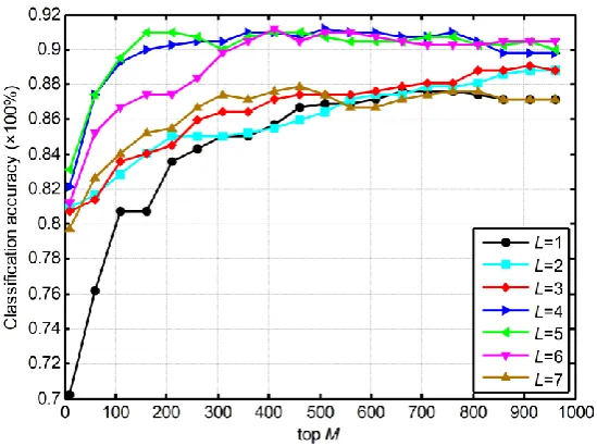
23
[image:23.595.159.434.213.418.2]off with the increase of L; (2) classification accuracy was improved and then stabilized in a certain range with the increase of M . Especially, when we fixed L to be 4 and then changed M from 360 to 810 with a stride of 50, the classification accuracy only varies in the range of [0.9048, 0.9119]. Consequently, we empirically set L4 and M 360 in all our subsequent land-use classification evaluations.
Fig. 8. Classification accuracy with different L and M .
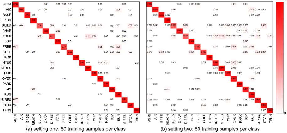
24
Fig. 9. Confusion matrix for experimental setting one and setting two, respectively.
[image:24.595.64.531.519.742.2]Table 1 presents the average classification accuracies of our method and some stat-of-the-art methods. The results of Table 1 expect for our method are all the best results from literatures of [3-7, 19, 20]. Their details can be found in [3-7, 19, 20]. Comparison with stat-of-the-art methods shows the huge performance gain resulting from our method (on average 8.62% and 12.72% for two different experimental setting). To our best knowledge, this result is the best on this data set, which adequately shows the effectiveness and superiority of this objectlets-based land-use classification approach.
Table 1 Average classification accuracies (%) of 12 different methods
Methods Number of training samples per class 50 (setting two) 80 (setting one)
Results from literatures
SSM-MF [4] 76 --
WD-BOVW [5] 87.38±1.27 --
MFJSC [19] 77.33 --
The method of [20] 79.2 -- The method of [3]
[3]
-- 81.67±1.23
BOVW [6] -- 76.81
BOVW+SCK [6] -- 77.71
Color-HLS [6] -- 81.19
Texture [6] -- 76.91
SPCK++ [7] -- 77.38
25
4.4 Sparselets-based land-use classification results and comparisons
To illustrate the availability of the proposed sparselets training framework, we evaluate the baseline method [23] and our proposed method based on our pre-trained object detectors on the 21 LULC classes data set [6, 7] using experimental one. In the rest of the paper, for simplicity, we will call the baseline sparselets learned by sparse coding method as SC-based sparselets, coarse sparselets learned by unsupervised single-hidden-layer auto-encoder as SA-based ones and fine sparselets learned by supervised single-hidden-layer neural network as SNN-based ones, respectively.
The total number of pre-trained object detectors, on all five held-out sets, used for sparselets training is N
3093,3140,3072,3110, 2822
. We define sparsity level as 10 K and set it to be the set of
0.95,0.9,0.8,0.7,0.6,0.5 , and set sparselets dictionary size
K to be the set of
100, 200,300 . Fig.
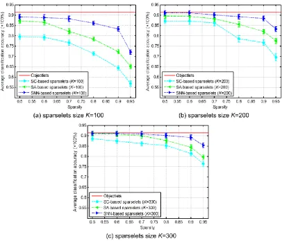
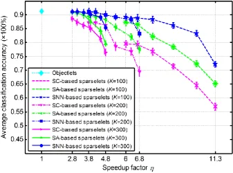
10 and Table 2 show the classification accuracy averaged over all five cross-validations obtained with different methods, different sparselets dictionary sizes, and different activation vector sparsity levels. Fig. 11 compares classification accuracy versus actual speedup factor, in which each curve shows results at six different sparsity levels: 0.5, 0.6, 0.7, 0.8, 0.9, and 0.95.
26
Fig. 10. Average classification accuracy obtained with different methods, different sparselets dictionary sizes and different activation vector sparsity levels.
Table 2 Average classification accuracies (%) with different methods and different sparsity levels Sparsity levels 0.95 0.9 0.8 0.7 0.6 0.5 Objectlets
K=100
SC 56.90±1.26 64.52±1.13 71.43±0.91 76.67±1.22 79.29±1.31 79.52±1.22
91.33±1.11 SA 65.12±1.05 72.34±1.12 78.46±0.91 82.18±1.21 86.53±1.32 87.29±1.25
SNN 72.12±1.06 83.23±1.10 86.15±0.93 88.23±1.22 88.84±1.32 89.12±1.21
K=200
SC 69.52±1.71 76.67±1.32 78.57±1.54 86.19±1.31 87.14±1.42 87.14±1.21 SA 77.51±1.21 82.06±1.12 85.56±1.26 88.29±1.32 89.38±1.41 89.45±1.16 SNN 83.23±1.23 88.35±1.16 89.21±1.13 90.04±1.23 91.03±1.24 91.08±1.17
K=300
[image:26.595.53.545.501.675.2]27
Fig. 11. Average classification accuracy and speedup factor obtained with different methods and different sparselets dictionary sizes, at six sparsity levels: 0.5, 0.6, 0.7, 0.8, 0.9, and 0.95.
5.
Conclusions
[image:27.595.128.466.59.309.2]28
state-of-the-art approaches demonstrate the effectiveness and superiority of our work.
References
[1] T. R. Martha, N. Kerle, C. J. van Westen, V. Jetten, and K. V. Kumar, “Segment optimization and data-driven thresholding for knowledge-based landslide detection by object-based image analysis,” IEEE Trans. Geosci. Remote Sens., vol. 49, no. 12, pp. 4928-4943, 2011.
[2] G. Cheng, L. Guo, T. Zhao, J. Han, H. Li, and J. Fang, “Automatic landslide detection from remote-sensing imagery using a scene classification method based on BoVW and pLSA,” Int. J. Remote Sens., vol. 34, no. 1, pp. 45-59, 2013.
[3] A. M. Cheriyadat, “Unsupervised Feature Learning for Aerial Scene Classification,” IEEE Trans. Geosci. Remote Sens., vol. 52, no. 1, pp. 439-451, 2014.
[4] Y. Zhang, X. Zheng, G. Liu, X. Sun, H. Wang, and K. Fu, “Semi-supervised manifold learning based multigraph fusion for high-resolution remote sensing image classification,” IEEE Geosci. Remote Sens. Lett., vol. 11, no. 2, pp. 464-468, 2014.
[5] L. Zhao, P. Tang, and L. Huo, “A 2-D wavelet decomposition-based bag-of-visual-words model for land-use scene classification,” Int. J. Remote Sens., vol. 35, no. 6, pp. 2296-2310, 2014.
[6] Y. Yang, and S. Newsam, “Bag-of-visual-words and spatial extensions for land-use classification,” in Proc. ACM SIGSPATIAL GIS, 2010, pp. 270-279.
[7] Y. Yang, and S. Newsam, “Spatial pyramid co-occurrence for image classification,” in Proc. IEEE Int. Conf. Comput. Vision, 2011, pp. 1465-1472.
29
[9] S. Bhagavathy, and B. S. Manjunath, “Modeling and detection of geospatial objects using texture motifs,” IEEE Trans. Geosci. Remote Sens., vol. 44, no. 12, pp. 3706-3715, 2006.
[10] X. Huang, L. Zhang, and L. Wang, “Evaluation of morphological texture features for mangrove forest mapping and species discrimination using multispectral IKONOS imagery,” IEEE Geosci. Remote Sens. Lett., vol. 6, no. 3, pp. 393-397, 2009.
[11] S. Xu, T. Fang, D. Li, and S. Wang, “Object classification of aerial images with bag-of-visual words,” IEEE Geosci. Remote Sens. Lett., vol. 7, no. 2, pp. 366-370, 2010.
[12] N. Longbotham, C. Chaapel, L. Bleiler, C. Padwick, W. J. Emery, and F. Pacifici, “Very high resolution multiangle urban classification analysis,” IEEE Trans. Geosci. Remote Sens., vol. 50, no. 4, pp. 1155-1170, 2012.
[13] Y. Chen, N. M. Nasrabadi, and T. D. Tran, “Hyperspectral image classification via kernel sparse representation,” IEEE Trans. Geosci. Remote Sens., vol. 51, no. 1, pp. 217-231, 2013.
[14] S. Moustakidis, G. Mallinis, N. Koutsias, J. B. Theocharis, and V. Petridis, “SVM-based fuzzy decision trees for classification of high spatial resolution remote sensing images,” IEEE Trans. Geosci. Remote Sens., vol. 50, no. 1, pp. 149-169, 2012.
[15] J. Munoz-Mari, D. Tuia, and G. Camps-Valls, “Semisupervised classification of remote sensing images with active queries,” IEEE Trans. Geosci. Remote Sens., vol. 50, no. 10, pp. 3751-3763, 2012.
[16] D. Tuia, M. Volpi, M. Dalla Mura, A. Rakotomamonjy, and R. Flamary, “Automatic feature learning for spatio-spectral image classification with sparse SVM,” IEEE Trans. Geosci. Remote Sens., DOI: 10.1109/TGRS.2013.2294724, 2014.
30 879-893, 2012.
[18] M. Kim, M. Madden, and T. A. Warner, “Forest type mapping using object-specific texture measures from multispectral Ikonos imagery: segmentation quality and image classification issues,” Photogramm. Eng. Remote Sens., vol. 75, no. 7, pp. 819-829, 2009.
[19] X. Zheng, X. Sun, K. Fu, and H. Wang, “Automatic annotation of satellite images via multifeature joint sparse coding with spatial relation constraint,” IEEE Geosci. Remote Sens. Lett., vol. 10, no. 4, pp. 652-656, 2013.
[20] B. Fernando, E. Fromont, and T. Tuytelaars, “Mining mid-level features for image classification,” Int. J. Comput. Vis., pp. 1-18, DOI : 10.1007/s11263-014-0700-1, 2014.
[21] F. F. Li, and P. Perona, “A bayesian hierarchical model for learning natural scene categories,” in Proc. IEEE Int. Conf. Comput. Vision Pattern Recognit., 2005, pp. 524-531.
[22] D. G. Lowe, “Distinctive image features from scale-invariant keypoints,” Int. J. Comput. Vis., vol. 60, no. 2, pp. 91-110, 2004.
[23] H. O. Song, S. Zickler, T. Althoff, R. Girshick, M. Fritz, C. Geyer, P. Felzenszwalb, and T. Darrell, “Sparselet models for efficient multiclass object detection,” in Proc. Eur. Conf. Comput. Vision, 2012, pp. 802-815.
[24] P. F. Felzenszwalb, R. B. Girshick, D. McAllester, and D. Ramanan, “Object detection with discriminatively trained part-based models,” IEEE Trans. Pattern Anal. Mach. Intell., vol. 32, no. 9, pp. 1627-1645, 2010.
[25] S. G. Mallat, and Z. Zhang, “Matching pursuits with time-frequency dictionaries,” IEEE Trans. Signal Process., vol. 41, no. 12, pp. 3397-3415, 1993.
31
[27] J. Mairal, F. Bach, J. Ponce, and G. Sapiro, “Online dictionary learning for sparse coding,” in Proc. IEEE Int. Conf. Machine Learning, 2009, pp. 689-696.
[28] D. E. Rumelhart, G. E. Hinton, and R. J. Williams, “Learning representations by back-propagating errors,” Nature, vol. 323, pp. 533-536, 1986.
[29] G. E. Hinton, and R. R. Salakhutdinov, “Reducing the dimensionality of data with neural networks,” Science, vol. 313, no. 5786, pp. 504-507, 2006.
[30] A. Ng, "CS294A lecture notes: Sparse autoencoder," Stanford University, 2010.
[31] P. Vincent, H. Larochelle, Y. Bengio, and P.-A. Manzagol, “Extracting and composing robust features with denoising autoencoders,” in Proc. Conf. Adv. Neural Inform. Process. Syst., 2008, pp. 1096-1103.
[32] J. Vogel, and B. Schiele, “Semantic modeling of natural scenes for content-based image retrieval,” Int. J. Comput. Vis., vol. 72, no. 2, pp. 133-157, 2007.
[33] N. Dalal, and B. Triggs, “Histograms of oriented gradients for human detection,” in Proc. IEEE Int. Conf. Comput. Vision Pattern Recognit., 2005, pp. 886-893.
[34] A. Hauptmann, R. Yan, W.-H. Lin, M. Christel, and H. Wactlar, “Can high-level concepts fill the semantic gap in video retrieval? A case study with broadcast news,” IEEE Trans. Multimedia, vol. 9, no. 5, pp. 958-966, 2007.
[35] S. Singh, A. Gupta, and A. A. Efros, “Unsupervised discovery of mid-level discriminative patches,” in Proc. Eur. Conf. Comput. Vision, 2012, pp. 73-86.
[36] C. Doersch, A. Gupta, and A. A. Efros, “Mid-level Visual Element Discovery as Discriminative Mode Seeking,” in Proc. Conf. Adv. Neural Inform. Process. Syst., 2013, pp. 494-502.
32
[38] J. Nocedal, “Updating quasi-Newton matrices with limited storage,” Math. Comput., vol. 35, no. 151, pp. 773-782, 1980.