City, University of London Institutional Repository
Citation
:
Nielsen, B. and Nielsen, J. P. (2014). Identification and forecasting in mortality
models. The Scientific World Journal, 2014, 347043 - ?. doi: 10.1155/2014/347043
This is the published version of the paper.
This version of the publication may differ from the final published
version.
Permanent repository link:
http://openaccess.city.ac.uk/4638/
Link to published version
:
http://dx.doi.org/10.1155/2014/347043
Copyright and reuse:
City Research Online aims to make research
outputs of City, University of London available to a wider audience.
Copyright and Moral Rights remain with the author(s) and/or copyright
holders. URLs from City Research Online may be freely distributed and
linked to.
Research Article
Identification and Forecasting in Mortality Models
Bent Nielsen
1,2,3and Jens P. Nielsen
41Department of Economics, University of Oxford, Oxford OX1 2JD, UK
2Programme on Economic Modelling, INET, University of Oxford, Oxford OX1 2JD, UK 3Nuffield College, Oxford OX1 1NF, UK
4Cass Business School, City University London, 106 Bunhill Row, London EC1Y 8TZ, UK
Correspondence should be addressed to Bent Nielsen; [email protected]
Received 22 January 2014; Accepted 17 April 2014; Published 2 June 2014
Academic Editor: Montserrat Guill´en
Copyright © 2014 B. Nielsen and J. P. Nielsen. This is an open access article distributed under the Creative Commons Attribution License, which permits unrestricted use, distribution, and reproduction in any medium, provided the original work is properly cited.
Mortality models often have inbuilt identification issues challenging the statistician. The statistician can choose to work with well-defined freely varying parameters, derived as maximal invariants in this paper, or with ad hoc identified parameters which at first glance seem more intuitive, but which can introduce a number of unnecessary challenges. In this paper we describe the methodological advantages from using the maximal invariant parameterisation and we go through the extra methodological challenges a statistician has to deal with when insisting on working with ad hoc identifications. These challenges are broadly similar in frequentist and in Bayesian setups. We also go through a number of examples from the literature where ad hoc identifications have been preferred in the statistical analyses.
1. Introduction
Mortality models are commonly used in a wide range of fields such as actuarial sciences, epidemiology, and sociology. They are often used in important decisions such as how to deal with unisex legislation in the pension industry; see Ornelas et al. [1] and Jarner and Kryger [2]. However, such models do often have inbuilt identification issues stemming from overparametrisation. While identification issues are omnipresent in statistical modelling, this paper focuses on mortality modelling, where estimated parameters are treated as time series and extrapolated to give forecasts of future mortality. The underlying theme of this paper is to provide strategies of avoiding arbitrariness resulting from the iden-tification process. We suggest two ways forward. First, we can reparametrise the model in terms of a freely varying parameter, which therefore has to be of lower dimension than the original parameter. Secondly, we can work with an identified version of the original parameter as long as we keep track of the consequences of the identification choice. That way we ensure that two researchers making different identification choices get the same statistical inferences and forecasts.
A simple example is the period model for an age-period array of mortality rates. It is well-known that the levels of the age- and period-effects cannot be determined from the likelihood representing the overparametrisation of the model. When the estimated age- and period-effects are treated as time series and subjected to plotting and extrapolation, then our approach ensures that the statistical analysis is the same for two researchers identifying the above model in two different ways. Whereas this issue is relatively simple for the age-period model, identification becomes more tricky for complicated models such as the age-period-cohort model and the model of Lee and Carter [3], let alone two-sample situations.
Mortality models are built as a combination of age, period, and cohort-effects, but the likelihood only varies with a surjective function of these time effects. The time effects can be divided into two parts. One part that moves the likelihood function and another part which does not induce variation in the likelihood function. We will argue that all inferences and forecasts should be concerned primarily with the part of the parameter that moves the likelihood function. This does not preclude the researcher from working with the time effects, but it gives some limitations on what can be done.
This is important because the motivation and the intuition of mortality models typically originate in the time effects. For instance, in the context of an age-period-cohort model linear trends cannot be identified so time series plots of the time effects need to be invariant to linear trends and extrapolations of time effects must preserve the arbitrary linear trend in the time effects. This applies regardless of whether the identification issue is dealt with in a frequentist manner or by Bayesian methods.
To formalise the discussion slightly return to the age-period example. Denote the predictor for the age-age-period data array by𝜇. The age-period model then determines how the predictor𝜇varies with a vector𝜃summarising age and period effects. That vector is split into two components 𝜉 and 𝜆 so that the predictor only depends on𝜃through𝜉but not on 𝜆 which cannot be identified by statistical analysis. In the age-period example𝜉could reflect the contrasts and the overall level of the predictor𝜇, whereas𝜆reflects the level of the age effect. The more principled solution is then to work exclusively with𝜉and simply consider𝜃as a motivation rather than the objective of the analysis. Another solution is to ad hoc identify𝜆based on a notion of mathematical convenience or based on a particular purpose given the substantive context.
Once an ad hoc identification of𝜆is chosen the identi-fication problem appears to go away, because the likelihood analysis can now go through. The reason is that the variation of𝜃is now reduced to the variation of𝜉precisely because𝜆 is fixed. Suppose two researchers choose the same likelihood and the same parametrisation of 𝜉 but different ad hoc identifications𝜆†and𝜆‡. Which of their conclusions will be the same and which will be different? As the likelihood only depends on𝜉the fits of the two researchers will be identical. But differences might arise if the statistical inference or forecasting or any other statistical analysis involves𝜆in some way.
Indeed, with many extrapolation methods forecasts will be invariant to the choice of 𝜆. But, there will also be extrapolation methods where this is not the case. Examples arise in the age-period-cohort model, where linear trends have to be handled with care.
We will start by analysing linearly parametrised models at a rather general level. We do this with two aspects in mind. First, we need to step back to a point in the analysis before ad hoc identification is made. Secondly, we also want to avoid the discussion of how to choose𝜉and 𝜆, which tend to be specific to the mortality model in question. Working at the general level we can focus on the mappings between different parametrisations and the invariance properties coming from these mappings. It is then seen that the parameter𝜉arises as a maximal invariant. The general setting also allows the formulation of a series of results discussing different types of ad hoc identification, first in a frequentist fashion and then in a Bayesian fashion.
Subsequently, we will consider the age-period-cohort model in detail, both for one- and two-sample situations. Using the general results it becomes easier to see that a number of popular methods inadvertently include features that are not invariant to ad hoc identification. These include
the “intrinsic estimator” advocated by Yang et al. [4], the “mixed model approach” by Yang and Land [5], the Bayesian approach by Berzuini and Clayton [6], and the two-sample analysis by Riebler and Held [7]. Finally, we consider the nonlinearly parametrised model of Lee and Carter [3]. The nonlinearity gives a further complication since the mapping from the time effects to the mortality predictor is nondif-ferentiable. As it turns out the mortality predictor varies in a smooth space, so the nondifferentiability is avoided by working directly with the mortality predictor instead of the original time effects. Instead, a Lee-Carter application should consider whether a certain matrix has rank of unity or zero. Apart from that the analysis is similar to that of linearly parametrised models. Likewise a theory is given for two-sample situations.
Throughout the paper our concern rests exclusively with the identification problem and the consequences of ad hoc identification for estimation, plots, inference, and forecasting. In practice, important additional concerns are how to choose appropriate models and forecasting methods. We would like to refer to Girosi and King [8], Pitacco et al. [9] for general discussions of these issues, and also to Kuang et al. [10] and Coelho and Nunes [11] for discussions of forecast methods in the light of structural breaks. Instead, the aim of the paper is to present an overall framework that can help streamlining the identification discussion that has appeared in so many papers in so many fields over so many years.
Section 2of this paper considers standard linear statistical models, which lend themselves to a relative straightforward analysis based on linear algebra. Any ad hoc identification splits the time effect into two components. The first com-ponent is an arbitrary comcom-ponent, which is not needed for the identification of the likelihood. The other component is necessary and sufficient to identify the model and hence sufficient for statistical analysis. InSection 3it is outlined how to analyze the statistical model when the latter component is ad hoc identified. It is argued that this can cause difficulties for estimation, interpretation, and forecast. InSection 4it is shown that Bayesian analysis shares the same challenges as the frequentist approach. In Sections5and 6we study the two particular examples: the omnipresent age-period-cohort and Lee-Carter mortality models. All proofs are collected in the Appendix.
2. Statistical Models with
Linear Parametrisations
In this section we present the identification problem in a linear framework. The problem is solved by analysing the mapping from the original time effect to the predictor which, in turn, leads to standard statistical analysis. In Section 6 we show how these ideas transfer to a nonlinear context. This contrasts with Section 3 in which we illustrate the analytical challenges and inconveniences arising from ad hoc identification.
is defined in Section 2.2 via the likelihood. In an over-parametrized linear model two different parameters might produce the same likelihood. InSection 2.3we analyze the mapping from the overparametrised parameter to the pre-dictor. This mapping enables us to split the overparametrised parameter into two. One arbitrary parameter and one param-eter identify the model without being overparametrised. This latter parameter is shown to be a maximal invariant param-eter. In Section 2.4 it is demonstrated how any statistical analysis can be based on this maximal invariant parameter alone. In particular we comment that visual data representa-tions, hypothesis testing, and forecasting are simple and well defined. This in turn leads to standard statistical analysis.
The analysis of the linearly parametrised involves pro-jections on linear or affine spaces and on their orthogonal complements. It is therefore convenient to introduce the following notation. A matrix𝑚has full column rank if𝑚𝑚 is invertible. In this case the orthogonal complement𝑚⊥ is a matrix so𝑚⊥𝑚 = 0and(𝑚, 𝑚⊥)is invertible. Thus, when
𝑚itself is invertible then𝑚⊥ is the empty matrix. It is not difficult to calculate𝑚⊥in practise, an explicit construction of𝑚⊥follows from a singular value decomposition of𝑚𝑚, choosing 𝑚⊥ as the eigenvectors associated with the zero eigenvalues. Moreover, let𝑚 = 𝑚(𝑚𝑚)−1so that𝑚𝑚is the identity matrix, while𝑚⊥= 𝑚⊥(𝑚⊥𝑚⊥)−1.
2.1. The Model. Think of the time effect𝜃 as our preferred intuitive, but unidentified parameter, and think of the pre-dictor 𝜇 as some function of 𝜃 specifying the model at hand. In a Poisson type model, where the mean specifies the distribution,𝜇could be the log of that mean. Such Poisson models are omnipresent in mortality models. We will often think of𝜃as containing some time effects. Often forecasting is carried out simply by isolating and extrapolating such a time effect.
Consider a data vector𝑌of dimension𝑛. This could, for instance, be the vector consisting of the stacked mortality rates for a rectangular age-period array of dimension𝐼 × 𝐽 in which case𝑛 = 𝐼𝐽. The statistical model for𝑌could be a generalized linear model. This involves an appropriately chosen distribution and a link function, which links the expected mortality rate to an𝑛-dimensional predictor, which is denoted by 𝜇. Taken together this defines a likelihood functionL(𝜇; 𝑌).
The model for the predictor𝜇is constructed in terms of, for instance, age, period, and cohort time effects. These time effects are summarized in a vector𝜃, which is of dimension
𝑞 < 𝑛. Therefore 𝜇 is a surjective function of 𝜃. For the moment the specification of the predictor is assumed linear so that
𝜇 = 𝐷𝜃 for𝜃 ∈ Θ =R𝑞, (1)
for some design matrix 𝐷 ∈ R𝑛×𝑞. We refer to this specification as the mortality model, while the space Θ is the time effect space. The time effect space is chosen as an unrestricted real space in accordance with the starting point of most mortality analyses.
The parameter space for the likelihood function and therefore for the statistical model is given by the range of variation for the predictor𝜇; that is,
𝑀 = (𝜇 ∈R𝑛: 𝜇 = 𝐷𝜃for𝜃 ∈ Θ =R𝑞) . (2)
The likelihood function is assumed uniquely identified on this space in the sense that for all pairs of predictors so𝜇† ̸= 𝜇‡ then the likelihood of𝜇†,𝜇‡differ; that is,
L(𝜇†; 𝑌) ̸=L(𝜇‡; 𝑌) , (3)
for𝑌in a set with positive probability.
2.2. The Identification Problem. The identification problem of mortality models arises when the mapping from the time effect spaceΘto the parameter space𝑀is surjective but not injective. With a linear parametrisation this arises when the design matrix𝐷has reduced column rank𝑝 < 𝑞so𝐷𝐷is singular. In this situation there exists time effects𝜃† ̸= 𝜃‡with the same likelihood:
L(𝐷𝜃†; 𝑌) =L(𝐷𝜃‡; 𝑌) , (4)
for all data𝑌. Then the time effect spaceΘis not useful as parameter space for the statistical model.
2.3. Analysing the Mapping 𝜃 → 𝜇. When analysing the mapping from our intuitively preferred parametrisation 𝜃 into the linear predictor𝜇, we will be able to rewrite𝜃as a sum of two components: one is a function of the predictor and the other is the arbitrary part varying with𝜃, but not with the predictor. We provide two methods for analysis.
The first method is to find a basis 𝑋 ∈ R𝑛×𝑝 with full column rank𝑝for the design 𝐷. The design matrix of the mortality model can then be expressed as𝐷 = 𝑋𝐴for some matrix𝐴 ∈ R𝑞×𝑝with full column rank𝑝. Introduce a new
𝑝-dimensional parameter:
𝜉 = 𝐴𝜃. (5)
The parameter space𝑀can then be written more parsimo-niously as
𝑀 = (𝜇 ∈R𝑛: 𝜇 = 𝑋𝜉 for𝜉 ∈R𝑝) . (6)
The mapping from𝜉to𝜇is bijective, so the statistical model can just as well be parametrised in terms of𝜉 ∈ Ξ =R𝑝.
Alternatively, the identification problem can be expressed through an invariance argument. This argument relates to the parameterization but resembles the classical invariance argument for reduction of data; see Cox and Hinkley [12, page 157]. With a linear parametrisation the argument involves the orthogonal complement to the matrix𝐴. That is a matrix
𝐴⊥ ∈ R𝑞×(𝑞−𝑝)which has the properties that𝐴
⊥𝐴 = 0and that(𝐴, 𝐴⊥)is invertible. The mortality model (1) is defined by the mapping
fromΘ = R𝑞 to𝑀. This mapping is surjective in that two different values of𝜃may result in the same𝜇and therefore the same likelihood. These equivalence classes in the time effect space can be described by the group of transformations
𝑔 : 𝜃 → 𝜃 + 𝐴⊥𝜁, (8)
acting onΘfor arbitrary𝜁 ∈R𝑞−𝑝. Indeed, it holds that𝜃and
𝑔(𝜃)will result in the same𝜇. The mapping (7) is therefore invariant to the group𝑔. We will argue that the parameter
𝜉 = 𝐴𝜃is a maximal invariant to the group𝑔acting onΘ, which provides a link with (6). It has to be argued that for any
𝜃†,𝜃‡ so that𝜉† = 𝐴𝜃†equals𝜉‡ = 𝐴𝜃‡ then𝜃‡ = 𝑔(𝜃†), see Cox and Hinkley [12, page 159]. For this argument use the orthogonal projection identity to write
𝜃 = 𝐴(𝐴𝐴)−1𝜉 + 𝐴⊥(𝐴⊥𝐴⊥)−1𝜑; (9)
for unique𝜉 = 𝐴𝜃and𝜑 = 𝐴⊥𝜃. Thus, if𝐴𝜃‡ = 𝐴𝜃†then
𝜃‡ = 𝑔(𝜃†)with𝜁 = 𝜑‡− 𝜑†= 𝐴⊥(𝜃‡− 𝜃†).
In applications it can be difficult to find a basis𝑋for the design𝐷. It can be easier to find a group𝑔and hence𝐴⊥ and then use this information to construct𝐴and a candidate basis𝑋 = 𝐷𝐴, noting that𝐷 = 𝑋𝐴. This argument leaves it to be proven that 𝑋 is a basis, or equivalently, that the suggested group𝑔actually describes the equivalence classes of the mapping from𝜃to𝜇.
It is useful to note that in the choices of𝑋, 𝐴only the spaces spanned by them are unique since𝑋𝐴 = 𝑋𝑚𝑚−1𝐴 for any invertible𝑚 ∈R𝑝×𝑝. Likewise, the maximal invariant
𝜉is only unique up to bijective transformations. This lack of uniqueness has no impact on the analysis of the likelihood albeit it influences interpretations.
2.4. Statistical Analysis Using the Maximal Invariant Param-eter. The statistical model parametrised with the maximal invariant parameter𝜉can be analysed by standard statistical techniques. This contrasts to a range of problems that arise when working with an ad hoc identified time effect 𝜃. In the following the relatively simple standard statistical analysis of the model parametrised by 𝜉is discussed with respect to likelihood theory, interpretation, plots, hypothesis testing, forecasting, and Bayesian analysis. In Sections 3 and 4we give an overview of the much more complicated theory underpinning models parametrised by the ad hoc identified time effect𝜃. Age-period-cohort examples follow inSection 5.
2.4.1. Exponential Family Theory. Suppose the likelihood is drawn from a generalized linear model based on an exponential family. Then the model is actually a regular exponential family where the maximal invariant parameter
𝜉is the canonical parameter since it is freely varying in a real space; see Barndorff-Nielsen [13, page 116]. This opens up for a wealth of convenient statistical properties such as a likelihood equation with a simple expression and explicit conditions for a unique solution. In contrast, ad hoc identified parameters are based on an injective mapping of the canonical parameter
𝜉into𝜃; see Sections3.1and3.2. It is then more difficult to fully exploit the exponential family theory.
2.4.2. Interpretation and Plots. The maximal invariant parameter𝜉varies freely inR𝑝. It can therefore be interpreted as the parameter of any standard statistical model. Since
𝜉is freely varying the coordinates of 𝜉can be interpreted independently. When𝜃 is a collection of time effects then
𝜉can be organised as a collection of time series. Since the coordinates of𝜉are freely varying the time series plots of the components of𝜉have the usual interpretation of time series. In contrast, ad hoc identified estimators are constrained to a
𝑝-dimensional subspaceΘ𝜆ofΘ =R𝑞, which is often affine but can be more complicated. A consequence is that plots are complicated to evaluate; seeSection 3.4.1.
2.4.3. Hypothesis Testing. Hypotheses are easily formulated and analysed when using the maximal invariant parametri-sation. An affine hypothesis that restricts𝜉to vary in a𝑝𝐻 -dimensional affine subspace can be formulated as 𝐻𝜉 =
𝜂 for known matrices 𝐻 ∈ R𝑝×(𝑝−𝑝𝐻), 𝜂 ∈ R𝑝−𝑝𝐻. This implies a restriction on the predictor𝜇 = 𝑋𝜉of (6). Form the orthogonal complement 𝐻⊥ and recall the orthogonal projection identity𝐼𝑛= 𝐻𝐻+ 𝐻⊥𝐻⊥so that𝜇 = 𝑋𝐻𝐻𝜉 +
𝑋𝐻⊥𝐻⊥𝜉. Introduce a𝑝𝐻-dimensional parameter𝜑 = 𝐻⊥𝜉, a design matrix𝑋𝐻 = 𝑋𝐻⊥, and an offset𝑍𝐻 = 𝑋𝐻𝜂. The restricted parameter space is
𝑀𝐻= (𝜇 ∈R𝑛 : 𝜇 = 𝑋𝐻𝜑 + 𝑍𝐻 for𝜑 ∈R𝑝𝐻) . (10)
In an exponential family context both the unrestricted model and the restricted model form regular exponential families. A variety of nice properties then follow for the estimators and the test statistics from the exponential family theory. Examples are given in Sections 5.3 and 5.5.3. In contrast, the hypothesis derived from restrictions on ad hoc identified parameters and the resulting degrees of freedom are compli-cated to analyse; seeSection 3.4.2.
2.4.4. Forecasting. Most often the objective of a mortality study is to forecast the future mortality. In the linear context,
𝜇 = 𝑋𝜉, this is done by extending the design 𝑋 and by extrapolating𝜉.
It is usually easy to extend the design𝑋into the forecast horizon. This involves the construction of a triangular block matrix with an appropriate number of extra rows correspond-ing to the data over the forecast horizon as well as extra columns representing the extra parameters that would be needed:
𝑋ℎ= (𝑋𝑋 0ℎ
1 𝑋ℎ2) . (11)
Extrapolating𝜉into a vector̃𝜉then gives the forecast
The extrapolation of the parameter𝜉can be done as follows. The estimated parameter, or part of it, can be thought of as a time series. Any forecast techniques from the time series literature applied directly to𝜉can be used, subject to the usual contextual considerations.
Ad hoc identified time effects can be extrapolated in a similar way; seeSection 3.4.3. This may, however, result in avoidable arbitrary effects in the forecast. Necessary and suffi-cient conditions for this eventuality are given for age-period-cohort models in Section 5.4.3. The practical examples are mainly Bayesian in nature and are discussed next.
2.4.5. Bayesian Analysis. The introduction of the canonical parameter shows that the likelihood, in Bayesian notation, is of the form𝑝(𝑦 | 𝜃) = 𝑝(𝑦 | 𝜉)where𝜉is freely varying. A purist Bayesian analysis can simply introduce a prior on the canonical parameter,𝑝(𝜉). This is updated in a straight forward way, resulting in the posterior𝑝(𝜉 | 𝑦) = 𝑝(𝑦 |
𝜉)𝑝(𝜉)/𝑝(𝑦).
In contrast, introducing a prior on ad hoc identified parameters gives various difficulties. Only parts of the prior are updated by the likelihood, so that it becomes unclear which information arises from the data and which infor-mation arises from the ad hoc identification. Moreover, avoidable arbitrariness is introduced in the forecast; see Section 4. Introduction of hyperparameters exacerbates the issue. Examples are given in Sections5.4.4,5.5.2, and6.1.6.
3. Working with the Time Effects
InSection 2we considered the situations where estimation, hypothesis testing a hypothesis, or forecasting is carried out using the canonical parameter. However, there might be situations, where the original time effect parametrisation is preferred, perhaps because it is felt that this parametrisation is particularly helpful in guiding the intuition. This requires ad hoc identification of the time effect . In this section we will guide the considerations a statistician that has to go through when insisting on an analysis based on some nonunique parametrisations. As in Section 2 we focus on linearly parametrised models. Specific examples follow in Sections5and6.
In Section 3.1 ad hoc identification is defined. As an example we consider a least squares estimation problem with collinear regressors inSection 3.2. For the age-period-cohort model reviewed inSection 5it is common to ad hoc identify in two steps: first identifying levels then the linear trends. We consider such two-step ad hoc identification inSection 3.3. The consequence of ad hoc identification is considered in Section 3.4. Indeed, when forecasting the time effect, we do not want the forecast to depend on the identification scheme. The same applies to graphical visualisation of our data, where the eye may extract patterns that depend on the identification scheme. Likewise, confusion may arise when formulating a hypothesis directly on the time effect parameters.
3.1. Ad Hoc Identification. In this section the time effect parametrisation is considered. An identification scheme has
to be introduced when working with the time effects. This may rest on mathematical convenience or it may be chosen for a particular purpose given the substantive context. We therefore call it ad hoc identification. Here we consider a simple identification scheme but turn to a more common two-step identification scheme inSection 3.3.
Once the canonical parameter𝜉has been estimated there is often a wish to return to the original time effect𝜃. The two are linked through the surjective mapping
𝜃 → 𝜉 = 𝐴𝜃, (13)
fromΘ = R𝑞toΞ = R𝑝. Indeed, since𝜉is constructed as a function of𝜃the notation for𝜉is often chosen to reflect
𝜃. The canonical parameter𝜉does, however, only give partial information about𝜃. The remaining part, say𝜆, of𝜃will have to be chosen by the researcher and combined with𝜉.
A linear ad hoc identification of 𝜃comes about by the researcher choosing a constraint
𝐿𝜃 = 𝜆 (14)
for some known𝜆 ∈ R𝑞−𝑝and some matrix𝐿 ∈ R𝑞×(𝑞−𝑝) chosen so the square matrix(𝐴, 𝐿) is invertible. The time effect spaceΘis now reduced to an affine subspace
Θ𝜆= (𝜃𝜆∈ Θ : 𝐿𝜃𝜆= 𝜆) . (15)
Given𝜃we can find𝜉,𝜆through (13) and (14) as(𝜉, 𝜆) =
(𝐴, 𝐿)𝜃. At the same time, given values of 𝜉, 𝜆 and the invertibility of(𝐴, 𝐿), the ad hoc identified time effect is found through
𝜃𝜆= (𝐴𝐿) −1
(𝜉𝜆) = 𝐿⊥(𝐴𝐿⊥) −1
𝜉 + 𝐴⊥(𝐿𝐴⊥)−1𝜆. (16)
In this notation a subindex𝜆is introduced to avoid confusion with the time effect𝜃in the original mortality model. Indeed, there are now four different parameters in play, namely, the original time effect𝜃 ∈ Θ, the predictor𝜇 ∈ 𝑀, the maximal invariant parameter𝜉 ∈ Ξ and the ad hoc identified time effect𝜃𝜆 ∈ Θ𝜆, each of which has a different interpretation. The mapping from 𝜃 to each of𝜇, 𝜉, and 𝜃𝜆 is surjective, while there are bijective mappings between the latter three. The interpretations of the time effect 𝜃 and the canonical parameter𝜉will inevitably be different. For a start they have different dimensions. Endowing the spaces with Euclidean norms shows that distances in the two spacesΘandΞwill be judged differently. The time effect𝜃and the ad hoc identified time effect 𝜃𝜆 will similarly have different interpretations. Although they have the same dimensions the Euclidean norms onΘandΘ𝜆will be rather different. Confusion may arise in the interpretation of a mortality analysis if there is no clear distinction between 𝜃 and 𝜃𝜆. In addition an unnecessary arbitrariness may arise when making inference on𝜃𝜆or extrapolating𝜃 ∈ Θ𝜆. We will return to these issues inSection 3.4.
in a linear fashion as in (14). Indeed it is common for Poisson models with a log link to ad hoc identify 𝜃 through the original multiplicative scale. That means that the ad hoc identification is done nonlinearly through
𝜉 = 𝐴𝜃
𝜆, 𝜆 = 𝑓 (𝜃𝜆) . (17)
The fit of the model is unaffected by the ad hoc identifica-tion. Indeed the fit is measured in terms of the estimate of the predictor𝜇 = 𝐷𝜃𝜆where𝐷 = 𝑋𝐴. Since the identification is made so𝜉 = 𝐴𝜃𝜆; the estimated predictor reduces to
̂𝜇 = 𝐷̂𝜃𝜆= 𝑋𝐴̂𝜃𝜆= 𝑋̂𝜉, (18) regardless of the choice of ad hoc identification.
3.2. A Least Squares Example. As an illustration of estimation in the presence of ad hoc identification consider a normal likelihood. Different, but equivalent, expressions can be found depending on the parametrisation. The likelihood of the predictor𝜇is
L(𝜇, 𝜎2; 𝑌) = (2𝜋𝜎2)−𝑛/2exp{− 1
2𝜎2(𝑌 − 𝜇)(𝑌 − 𝜇)} for𝜇 ∈ 𝑀, 𝜎2> 0.
(19)
Rewriting it in terms of the canonical parameter it is
L(𝜉, 𝜎2; 𝑌) = (2𝜋𝜎2)−𝑛/2exp{− 1
2𝜎2(𝑌 − 𝑋𝜉)(𝑌 − 𝑋𝜉)} for𝜉 ∈ Ξ =R𝑝, 𝜎2> 0,
(20)
while introducing the time effect parameter gives
L(𝜃, 𝜎2; 𝑌)
= (2𝜋𝜎2)−𝑛/2exp{− 1
2𝜎2(𝑌 − 𝑋𝐴𝜃)
(𝑌 − 𝑋𝐴𝜃)}
for𝜃 ∈ Θ =R𝑞, 𝜎2> 0. (21)
The likelihood (20) of the canonical parameter 𝜉 can be analysed by the least squares method since the design𝑋has full column rank. The maximum likelihood estimator for𝜉 and the predictor for the data are
̂𝜉 = (𝑋𝑋)−1𝑋𝑌, ̂𝑌 = 𝑋̂𝜉 = 𝑋(𝑋𝑋)−1𝑋𝑌. (22) Along with the residual variance this is all the information that is given by the likelihood.
The likelihood (21) of the time effect𝜃only depends on
𝜃through𝜉 = 𝐴𝜃. The lack of identification means that the maximum likelihood estimator for𝜃has an arbitrary element, so that it is a set valued estimator. Based on (16) this can be expressed by
̂
Θ𝜆= 𝐿⊥(𝐴𝐿⊥)−1̂𝜉 + 𝐴⊥(𝐿𝐴⊥)−1𝜆
where ̂𝜃𝜆∈ Θ𝜆⊂ Θ,
(23)
for any𝐿so(𝐴, 𝐿)is invertible and for any𝜆 ∈R𝑞−𝑝. The fit, however, remains the same and (18) becomes
̂𝜇 = 𝐷̂𝜃𝜆= 𝑋𝐴{𝐿⊥(𝐴𝐿⊥)−1̂𝜉 + 𝐴⊥(𝐿𝐴⊥)−1𝜆}
= 𝑋̂𝜉 = ̂𝑌.
(24)
In order to compute actual estimates then𝐿, 𝜆 have to be chosen, which amounts to ad hoc identification. For instance, with the ad hoc identifying restrictions 𝐿 = 𝐴⊥ and 𝜆 =
0then ̂𝜃𝜆 can be thought of as the least squares estimator of 𝑌 on 𝐷 using the Moore-Penrose generalised inverse for the singular matrix𝐷𝐷; see Searle [14, page 212]. See Section 5.4.1for an example.
3.3. Step-Wise Identification. It is common to ad hoc identify parameter in a step-wise fashion. In the first step the time effect parameter is only partially constrained. The full iden-tification then follows in a second step. An example is given inSection 5.4.1for an age-period-cohort model in which the levels of the time effects are constrained in the first step leaving the ad hoc identification of the linear trends to the second step.
The first step constraints are affine of the type
𝐶𝜃𝐶= 𝜓, (25)
for known matrices𝐶 ∈ R𝑞×(𝑞−𝑞𝐶), 𝜓 ∈ R𝑞−𝑞𝐶. The con-strained time effect space is then
Θ𝐶= (𝜃𝐶∈ Θ : 𝐶𝜃𝐶= 𝜓) . (26)
Thereby the𝑞-dimensional time effect spaceΘis reduced to a𝑞𝐶-dimensional variation. The properties of this partially ad hoc identified parameter space depends on the rank of the matrix (𝐴, 𝐶). If the number of constraints, 𝑞 − 𝑞𝐶, is at most equal to the number of unidentified components
𝑞 − 𝑝, it is possible that (𝐴, 𝐶) has full column rank. In that case the constraint implies a partial ad hoc identification without constraining the parameter space𝑀of the statistical model. This is shown in Theorem 1; see also Section 5.4.1 for an example, while the proof is given in the Appendix. When(𝐴, 𝐶)has reduced rank the parameter space𝑀is also constrained; seeSection 3.4.2for a discussion.
Theorem 1. Suppose (𝐴, 𝐶)has full column rank. Then the matrix𝑚 = 𝐴⊥𝐶 ∈ R(𝑞−𝑝)×(𝑞−𝑞𝐶)has full column rank and the constraint(25)does not constrain the canonical parameter
𝜉and the predictor𝜇. Hence, the predictor space remains of the form(2). The equivalence classes inΘ𝐶under the mapping
𝜃 → 𝜇 = 𝑋𝐴𝜃are given by the group
𝑔𝐶: 𝜃 → 𝜃 + 𝐴⊥𝑚⊥𝜁, (27)
for arbitrary 𝜁 ∈ R𝑞𝐶−𝑝 where 𝑚
⊥ ∈ R(𝑞−𝑝)×(𝑞𝐶−𝑝) is the
orthogonal complement of𝑚. The maximal invariant remains
𝜉 = 𝐴𝜃.
relative to the constrained spaceΘ𝐶rather than the spaceΘ. This is awkward as discussed inSection 3.4below. It is also considerably more complicated than working with the freely varying canonical parameter𝜉; seeSection 2.4.2.
3.4. Consequences of Ad Hoc Identification. In the following we will look closer at the consequences of working with the ad hoc identified time effect parameter𝜃in the context of a linear mortality model of the form 𝜇 = 𝐷𝜃. We consider the consequences for plotting, hypothesis testing, and forecasting.
3.4.1. Plots of Time Effects. In the mortality model (1) the time effect𝜃is the concatenation of age, period, and cohort effects. It seems natural to think of these individual time effects as time series and to plot them against time. As the time effect𝜃 varies in the unrestricted spaceΘ =R𝑞this maps the𝑞-vector into unrestricted time series.
Estimates of the time effects are constructed by combin-ing an estimate of𝜉with an ad hoc chosen value for𝜆 = 𝐿𝜃, see (14). The resulting estimate ̂𝜃𝜆 is therefore constrained to the spaceΘ𝜆 ⊂ Θ. The interpretation of the estimate ̂𝜃𝜆 is therefore different from the interpretation of the original time effect𝜃. Distances on the spacesΘandΘ𝜆 are judged differently and the variability of ̂𝜃𝜆 is deduced exclusively from̂𝜉through (16). The time series components of ̂𝜃𝜆 are now restricted through𝜆 = 𝐿𝜃𝜆. Plots of thê𝜃𝜆-time series are therefore interpreted differently from the imagined plots of the original𝜃-time series and from the plots of the maximal invariant parameter𝜉discussed inSection 2.4.2. Indeed, if one were to analyse the estimated̂𝜃𝜆-time series statistically the linear constraint should be taken into account. This is a bit complicated as illustrated below, but it is the consequence of working with the ad hoc identified parameter𝜃𝜆rather than the canonical parameter𝜉.
Attempts to give intrinsic meaning to𝜆will be specific to the index set for the data set at hand. For instance, the requirement that the age effect should be zero on average does not carry over when looking at a subsample or when forecasting. It is not obvious that such an ad hoc identification is any more or less arbitrary than saying that, for instance, the first or the last age effect should have a particular value.
Adding confidence bands to a plot of ̂𝜃𝜆 is in itself not difficult. If ̂𝜉 is asymptotically normal with mean 𝜉 and variance Σ, then ̂𝜃𝜆 is asymptotically normal with mean
𝜃𝜆 and variance𝐿⊥(𝐴𝐿⊥)−1Σ(𝐿⊥𝐴)−1𝐿⊥. This is a normal distribution on the space Θ𝜆. The interpretation of these standard errors will therefore be similar to that of̂𝜃𝜆itself.
Finally, it may be of interest to analyse the estimated̂𝜃𝜆 -time series statistically. Denote this -time series by 𝑥𝜆. Its sample space is nowΘ𝜆. A statistical model onΘ𝜆 can be built as follows. The starting point could be a time series model for unrestricted variables 𝑥on the sample space Θ. This gives a joint density for𝑥 ∈ Θ, which can be reduced by marginalisation to a density for𝑥𝜆 ∈ Θ𝜆. Whether one is working with the unrestricted model for𝑥 ∈ Θ or the
restricted model for𝑥𝜆∈ Θ𝜆inferences that are invariant to𝑔 must be based on those statistics of𝑥or𝑥𝜆that are invariant to𝑔. Thus, inferences must be based on the maximal invariant under𝑔. For a general overview of invariant reduction see Cox and Hinkley [12, page 175f], whereas Nielsen [15] gives the argument in some detail for an autoregression with a linear trend.
3.4.2. Hypothesis Testing. Having formulated the model in terms of time effects it may be of interest to test the hypothesis that one of these time effects is absent. No identification issues arise when the hypothesis is formulated as a restriction on the canonical parameter𝜉as discussed inSection 2.4.3. But one has to be careful when formulating hypotheses in terms of the original time effect. See Sections5.4.5,5.5.3, and5.5.4for examples.
Affine hypotheses on the time effect are of the form
𝑅𝜃𝑅= 𝜌, (28)
for known matrices𝑅 ∈R𝑞×(𝑞−𝑞𝑅),𝜌 ∈R𝑞−𝑞𝑅. The constrained time effect space is then
Θ𝑅= (𝜃𝑅∈R𝑞 : 𝑅𝜃𝑅= 𝜌) . (29)
To see how the restriction (28) restricts the predictor space
𝑀 ⊂R𝑛recall that the predictor𝜇only depends on𝜃through
𝜉 = 𝐴𝜃. Thus, the analysis of the restriction (28) depends on the interplay between the matrices𝐴,𝑅.Theorem A.3in Appendix A.3gives a general result to that effect. It shows that the hypothesis (28) restricts the predictor space𝑀to a𝑝𝑅 -dimensional affine subspace ofR𝑛in so far as it restricts the canonical parameter𝜉. In particular, the degrees of freedom of the hypothesis,𝑝 − 𝑝𝑅, may in general be different from the dimension reduction of the time effect parameter,𝑞 − 𝑞𝑅. When this is the case the restriction (28) has an element of ad hoc identifying the time effect.
3.4.3. Forecasts. Forecasts can be made by extrapolating the ad hoc identified time effects𝜃𝜆. Two researchers choosing different ad hoc identification schemes, but otherwise making the same analysis, may make different forecasts. This can be avoided if the extrapolation method is chosen with some care. Following the linear approach outlined in Section 2.4.4 the predictor𝜇 = 𝐷𝜃 = 𝑋𝐴𝜃is forecasted by extending the design𝐷into
𝐷ℎ= (𝐷𝐷 0ℎ
1 𝐷ℎ2) . (30)
Extrapolating the ad hoc identified𝜃𝜆into a vector(𝜃𝜆, ̃𝜃𝜆) then gives the forecast
̃𝜇 = (𝐷ℎ1, 𝐷2ℎ) (𝜃𝜆
̃𝜃𝜆) = 𝐷ℎ1𝜃𝜆+ 𝐷ℎ2̃𝜃𝜆. (31)
ad hoc identification may cancel each other so that the overall forecast ̃𝜇is invariant to the ad hoc identification. Such invariance would seem desirable in most applications unless there is strong substantial reason for the ad hoc identification scheme. Necessary and sufficient conditions for invariance are presented for the age-period-cohort model in Section 5.4.3and for a nonlinear model inSection 6.1.5.
In contrast, these considerations are redundant when working with the canonical parameter,𝜉; seeSection 2.4.4.
4. Bayesian Models and Random
Effects Models
Mortality analysis is often carried out using either Bayesian methods or random effects methods. The mortality model is then altered through the introduction of a prior distribution on the parameters. One might think that the identification problems become less of an issue or even disappear. This is not the case since the Bayesian method and the random effects method is based on the mortality likelihood which only depends on the time effect𝜃through the maximal invariant parameter𝜉. Thus, the identification challenges remain. The issue is that a prior on the unidentified part, say𝜆, of the time effect amounts to an ad hoc identification. Indeed, the conditional prior of𝜆given𝜉is not updated by the mortality likelihood. A main difference is that a maximum likelihood analysis of the original mortality likelihood usually prompts the researcher when there is an identification issue, whereas both Bayesian methods and random effects methods allow computations to go through despite an identification issue.
InSection 4.1it is seen that introduction of a conditional prior on𝜆given𝜉is the Bayesian analogue of ad hoc identi-fication. This leads to the same type of forecasting challenges as in the frequentist settings as is seen in Section 4.2. In Section 4.3we show how the Bayesian identification issues transfer to random effects models.
4.1. Bayesian Estimation. For Bayesian and random effects models we formulate a likelihood and a prior. Thus, consider a likelihood𝑝(𝑦 | 𝜃) = 𝐿(𝜃; 𝑦). Replacing 𝜃 by 𝜉, 𝜆 the identification problem implies that
𝑝 (𝑦 | 𝜉, 𝜆) = 𝑝 (𝑦 | 𝜉) for all outcomes𝑦. (32) The prior on𝜃is factorised as𝑝(𝜃) = 𝑝(𝜉, 𝜆) = 𝑝(𝜉)𝑝(𝜆 |
𝜉). In the case of Bayesian estimation the following result emerges.
Theorem 2. Suppose the likelihood satisfies(32). Then (i)the predictive distribution does not depend on the
con-ditional prior for𝜆:
𝑝 (𝑦) = ∫ 𝑝 (𝑦 | 𝜉) 𝑝 (𝜉) 𝑑𝜉; (33)
(ii)the posterior satisfies
𝑝 (𝜉 | 𝑦) = 𝑝 (𝑦 | 𝜉) 𝑝 (𝜉)
𝑝 (𝑦) , 𝑝 (𝜆 | 𝜉, 𝑦) = 𝑝 (𝜆 | 𝜉) ;
(34)
(iii)the posterior means satisfy
𝐸 (𝜉 | 𝑦) = ∫ 𝜉𝑝 (𝜉 | 𝑦) 𝑑𝜉,
𝐸 (𝜆 | 𝜉, 𝑦) = 𝐸 (𝜆 | 𝜉) ,
𝐸 (𝜆 | 𝑦) = ∫ 𝐸 (𝜆 | 𝜉) 𝑝 (𝜉 | 𝑦) 𝑑𝜉.
(35)
Theorem 2shows that it suffices to give a prior to𝜉and ignore𝜆as advocated inSection 2.4.5. Indeed the conditional prior for 𝜆 given 𝜉 is not updated. Theorem 2 appears to be well-known; see Poirier [16, Proposition 2] or Smith [17, Section B].
Due to Theorem 2the Bayesian analyst faces the com-plications outlined inSection 3.4. Indeed, suppose that two Bayesian researchers choose the same likelihood𝑝(𝑥 | 𝜉, 𝜆) =
𝑝(𝑥 | 𝜉) and the same prior 𝑝(𝜉) for 𝜉, but different conditional priors for𝜆given𝜉. Their marginal distributions for the data are identical, but any inferences regarding interpretation or forecasting will differ in so far as they involve the unidentified parameter𝜆. A Bayesian researcher should therefore be cautious with inference related to𝜆. There will of course be situations where the prior knowledge of
𝜆 given 𝜉is found to be of substantive relevance. In such situations it seems more fruitful to change the likelihood to include that information.
4.2. Forecasting. Bayesian forecasts involve integrating an extrapolative distribution. This can be done in two ways, either working exclusively with the identified, maximal invariant parameter𝜉as inSection 2.4.4, or working with the time effect𝜃 = (𝜉, 𝜆)as inSection 3.4.3.
4.2.1. Forecasting Using the Maximal Invariant Parameter. Consider first the case where only the maximal invariant parameter𝜉is used. In that case the forecast is computed by sampling from the posterior𝑝(𝜉 | 𝑦)and then extrapolating̃𝜇 using the sampled value𝜉using some extrapolative methods, say𝑝(̃𝜇 | 𝜉, 𝑦). In combination this gives the forecast
𝑝 (̃𝜇 | 𝑦) = ∫ 𝑝 (̃𝜇 | 𝜉, 𝑦) 𝑝 (𝜉 | 𝑦) 𝑑𝜉. (36)
4.2.2. Forecasting Using the Ad Hoc Identified Time Effect. Consider now forecasts involving the full time effect 𝜃 =
(𝜉, 𝜆).Theorem 2(ii) shows that the posterior satisfies𝑝(𝜃 |
𝑦) = 𝑝(𝜉 | 𝑦)𝑝(𝜆 | 𝜉). The distribution forecast with extrapolation𝑝(̃𝜇 | 𝜉, 𝜆, 𝑦)is then
𝑝 (̃𝜇 | 𝑦) = ∬ 𝑝 (̃𝜇 | 𝜉, 𝜆, 𝑦) 𝑝 (𝜉 | 𝑦) 𝑝 (𝜆 | 𝜉) 𝑑𝜆 𝑑𝜉. (37)
The concern is now as follows. Suppose a second researcher chooses the same extrapolative method, likelihood, and prior for𝜉, but different conditional priors𝑝†(𝜆 | 𝜉). In general, this will result in a different distribution forecast:
The question is then under which conditions will𝑝(̃𝜇 | 𝑦) =
𝑝†(̃𝜇 | 𝑦)so that the distribution forecasts are invariant to the choice of conditional prior for𝜆 given 𝜉? A sufficient condition is that the extrapolation method does not depend on𝜆so
𝑝 (̃𝜇 | 𝜉, 𝜆, 𝑦) = 𝑝 (̃𝜇 | 𝜉, 𝑦) . (39)
Condition (39) could alternatively be expressed as requiring that the forecast𝑝(̃𝜇 | 𝜃, 𝑦) = 𝑝(̃𝜇 | 𝜉, 𝜆, 𝑦)is invariant to the group𝑔acting on the time effect spaceΘso that𝑝(̃𝜇 |
𝜉, 𝜆, 𝑦) = 𝑝{̃𝜇 | 𝜉, 𝑔(𝜆), 𝑦}.
Theorem 3. Suppose that the likelihood satisfies(32)and the priors are probabilities. If the extrapolative distribution does not depend on𝜆so(39)holds; then the forecast distribution
𝑝(̃𝜇 | 𝑦) computed in (37) is invariant to the choice of conditional prior for𝜆given𝜉. The forecast then reduces to(36).
To summarise, the identification issues surrounding Bayesian analysis are similar to those outlined in the pre-vious sections. Examples of the problems that can arise are discussed in Sections5.4.4, 5.5.2, and6.1.6. There are two solutions to the identification problem. The first is only to formulate a prior on𝜉; seeSection 2.4.5. Incidentally, this is what Bernardo and Smith [18, page 218] do in their discussion of the two-way analysis of variance, albeit without linking it to the considerations of Smith [17]. The prior𝑝(𝜉)can of course be constructed by formulating a prior on𝜃and then reduce it to a prior on𝜉by marginalisation so𝑝(𝜉) = ∫ 𝑝(𝜉, 𝜆)𝑑𝜆. The other solution is to work with a prior on𝜃but avoid those parts of the posterior that depend on𝜆.
4.3. Random Effects Models. It is common to combine mortality models with a random effects approach, which effectively forms a new model. An example is given in Section 5.4.6. We consider the consequence of the lack of identification.
The random effect models are typically constructed as follows. Suppose the density of the data 𝑦 given the time effects 𝜃 = (𝜉, 𝜆)is of the form𝑝(𝑦 | 𝜉, 𝜆) = 𝑝(𝑦 | 𝜉) as before; see (32). A prior 𝑝(𝜃 | 𝜓) is chosen that now depends on a parameter𝜓. The prior can be decomposed as
𝑝(𝜃 | 𝜓) = 𝑝(𝜉 | 𝜓)𝑝(𝜆 | 𝜉, 𝜓).Theorem 2implies that the density of the data𝑦given𝜓is
𝑝 (𝑦 | 𝜓) = ∫ 𝑝 (𝑦 | 𝜉) 𝑝 (𝜉 | 𝜓) 𝑑𝜉. (40)
This in turn is used to form the random effects likelihood of
𝜓as
𝐿RE(𝜓 | 𝑦) = 𝑝 (𝑦 | 𝜓) . (41)
This, effectively, defines a new model. The random effects likelihood only depends on the prior𝑝(𝜃 | 𝜓)through𝑝(𝜉 |
𝜓). Two researchers choosing the same prior𝑝(𝜉 | 𝜓)but different conditional priors𝑝(𝜆 | 𝜉, 𝜓)will then get the same random effects likelihood and the same maximum likelihood estimator ̂𝜓.
In mortality modelling it is common to go one step further and estimate the time effects 𝜃 through the mean of the posterior𝑝(𝜃 | 𝑦, 𝜓)evaluated at𝜓 = ̂𝜓. Then the identification problem may show up.Theorem 2shows that
𝑝 (𝜉 | ̂𝜓, 𝑦) = 𝑝 (𝑦 | 𝜉) 𝑝 (𝜉 | ̂𝜓) 𝑝 (𝑦 | ̂𝜓) , 𝑝 (𝜆 | 𝜉, ̂𝜓, 𝑦) = 𝑝 (𝜆 | 𝜉, ̂𝜓) ,
(42)
so that the prior for 𝜉 is updated, while the conditional posterior for𝜆given𝜉is not updated by the data. Thus, in general the estimate for𝜃is based, in part, on a prior which is not updated by the data.
5. Age-Period-Cohort Models
We will now apply the theoretical considerations to analyse the age-period-cohort model. The methodological literature on this model is large and the consequences of the above theory are wide ranging.
In Section 5.1 we present the age-period-cohort model along with the maximal invariant parameter. This maximal invariant parameter is also called the canonical parameter because the age-period-cohort model is usually implemented as an exponential family; seeSection 2.4.1. When formulating the model we choose a notation matching the age-period-cohort literature rather than the reserving literature. At the same time the exposition takes it starting point in Kuang et al. [19], but the notation deviates.
The implementation of the canonical parameter depends on the type of data array. In Section 5.2 design matrices are given for age-cohort, age-period, and period-cohort data arrays. While they illustrate interesting differences in the structure for these data arrays, they also provide the basis for an immediate implementation via any generalised linear model software. The age-cohort model is expressed as a hypothesis of the age-period-cohort model in Section 5.3. Time effects and forecasting are considered inSection 5.4, while the two-sample age-period-cohort model is discussed inSection 5.5.
5.1. The Model and the Canonical Parameter. Here the age-period model is set up and a quite general identification result is reported.
Consider data𝑌𝑖𝑗indexed by(𝑖, 𝑗) ∈Iwhere𝑖is the age and𝑗is the period. The index set may be a rectangle given by
𝑖 = 1, . . . , 𝐼and𝑗 = 1, . . . , 𝐽so that the cohort𝑘 = 𝐼−𝑖+𝑗runs from1to𝐾 = 𝐼 + 𝐽 − 1. More generally, the index set could be a generalized trapezoid where two corners are cut off the rectangle so that the cohort𝑘runs from1+ℎ1to𝐼+𝐽−1−ℎ2for someℎ1, ℎ2 ≥ 0. The class of generalized trapezoids includes the three types of Lexis diagrams discussed by Keiding [20]. We will return to those special cases below.
The statistical model is defined by the assumption that the variables𝑌𝑖𝑗are independent with an exponential family distribution with predictor𝜇𝑖𝑗given by
The time effect𝜃 = (𝛼1. . . , 𝛼𝐼, 𝛽1, . . . , 𝛽𝑗, 𝛾ℎ1+1, . . .,𝛾𝐼+𝐽−1−ℎ2,
𝛿)now varies in some time effect spaceΘ ∈ R𝑞where𝑞 =
𝐼 + 𝐽 + 𝐾 + 1 − ℎ1− ℎ2.
The model (43) is of the form (1) discussed inSection 2. Specifically, the predictors𝜇𝑖𝑗 can be stacked in a vector𝜇 of dimension𝑛 = dimIand written as𝜇 = 𝐷𝜃. Thus, the parameter space for the model is of the form𝑀 = (𝜇 ∈
R𝑛 : 𝜇 = 𝐷𝜃for𝜃 ∈ Θ)as outlined in (2). The mapping
𝜃 → 𝜇 from Θ to 𝑀 is surjective and the equivalence classes in the time effect space can be described by a group of transformations that are discussed in (8). This group can be represented as
𝑔 : ( 𝛼𝑖
𝛽𝑗
𝛾𝑘 𝛿
) → (
𝛼𝑖+ 𝑎 + (𝑖 − 1) 𝑑 𝛽𝑗+ 𝑏 − (𝑗 − 1) 𝑑 𝛾𝑘+ 𝑐 + (𝑘 − 1) 𝑑 𝛿 − 𝑎 − 𝑏 − 𝑐 − (𝐼 − 1) 𝑑
) for𝜃 ∈ Θ,
(44)
for any 𝑎, 𝑏, 𝑐, and 𝑑. This is of the form (8) with 𝜁 =
(𝑎, 𝑏, 𝑐, 𝑑)although the definition of the matrix𝐴depends on the structure of the index setI.
A first clue for the canonical parametrisation is given by Fienberg and Mason [21] and Clayton and Schiffler [22] who pointed out that, on the multiplicative scale, ratios of relative risks are invariant. On the additive scale this amounts to looking at second differences, such asΔ2𝛼𝑖 = 𝛼𝑖 − 2𝛼𝑖−1 +
𝛼𝑖−2. A graphical illustration of the double differences is given inFigure 1 (graphics were done using R 3.0.2, see R Development Core Team [23]), which is taken from Miranda et al. [24]. Panel (a) illustrates the interpretations of the formula for Δ2𝛼𝑖 as follows. Consider the 1970 and 1971 cohorts. In 2010 these have ages 40 and 39, while in 2011 these have ages 41 and 40. Thus,Δ2𝛼41represents the increase in mortality from ages 40 to 41 in 2011 relative to the increase from ages 39 to age 40 in 2010. An equivalent interpretation is that which represents the increase in mortality from ages 40 to 41 for the 1970 cohort relative to the increase from ages 39 to 40 for the 1971 cohort. In a similar way panels (b) and (c) illustrate the formulas forΔ2𝛽2012andΔ2𝛾1972.
Kuang et al. [19] introduces a parameter formed by these second differences as well as three entries of the predictor; that is,
𝜉 = (𝜇𝑖1𝑗1, 𝜇𝑖2𝑗2, 𝜇𝑖3𝑗3, Δ2𝛼3, . . . , Δ2𝛼𝐼, Δ2𝛽3, . . . , Δ2𝛽𝐽,
Δ2𝛾ℎ1+3, . . . , Δ2𝛾𝐾−ℎ2) . (45)
The parameter𝜉varies in the spaceΞ =R𝑝where𝑝 = 𝑞 −
4. If the three points𝜇𝑖1𝑗1, 𝜇𝑖2𝑗2, and𝜇𝑖3𝑗3 are chosen not to be linearly related then they define the levels and the linear trends in the predictor. The formal condition is that a certain determinant defined from the indices is nonzero; that is,
𝑖2𝑗3− 𝑖3𝑗2+ 𝑖3𝑗1− 𝑖1𝑗3+ 𝑖1𝑘2− 𝑖2𝑘1 ̸= 0. (46)
Theorem 4 (see [19], [25, Corollary 2]). Let 𝜇 satisfy(43). If the condition(46)is satisfied then the parameter𝜉of (45) satisfies the following:
(i)𝜉is a function of𝜃which is invariant to the group𝑔in (44);
(ii)𝜇is a function of𝜉;
(iii)the parametrisation of𝜇by𝜉is exactly identified in that
𝜉† ̸= 𝜉‡⇒ 𝜇(𝜉†) ̸= 𝜇(𝜉‡).
Theorem 4 therefore shows that𝜉 varies freely in Ξ =
R𝑝. Moreover, 𝜉is a maximal invariant of the mapping𝑚 from𝜃to𝜇under the transformations𝑔. It should be noted that the choice of maximal invariant is not unique. Indeed, any bijective mapping of𝜉can serve as maximal invariant. The choice of𝜉is convenient since it becomes the canonical parameter in generalized linear models of the exponential family type.
In itself this theorem does not tell how to express the predictor𝜇in terms of the canonical parameter𝜉. The link depends on the structure of the index set I. The above mentioned paper gives implicit expressions for generalized trapezoid index sets. In the following we report explicit expressions for the 3 principal Lexis diagrams.
5.2. Design Matrices for Lexis Diagrams. The link between the canonical parameter𝜉and the predictor 𝜇is analysed for the 3 principal Lexis diagrams. We start with age-cohort data arrays, which were the focus of attention in Kuang et al. [19]. Such arrays are easiest to analyse because all three time scales increase from the point where𝑖 = 𝑗 = 𝑘 = 1. As a consequence the results are relatively easier for these arrays.
5.2.1. Age-Cohort Data Arrays. Age-cohort data arrays are rectangular in the age and cohort indices and given by
Iac= {(𝑖, 𝑘) : 𝑖 = 1, . . . , 𝐼, 𝑘 = 1, . . . , 𝐾} . (47)
Consequently, the period index𝑗 = 𝑖 + 𝑘 − 1varies over𝑗 =
1, . . . , 𝐽 = 𝐼 + 𝐾 − 1. Keiding [20] refers to this Lexis diagram as the first principal set of death.
Age-cohort arrays are in particular used for reserving in general insurance. In that situation, only the triangle1 ≤
𝑖, 𝑗, 𝑘 ≤ 𝐼is observed. The issue is to forecast the other triangle in the square1 ≤ 𝑖, 𝑘 ≤ 𝐼. In the reserving literature these triangles are referred to as the upper and lower triangles, since the cohort axis has reverse order. The two-factor age-cohort model for triangular age-cohort arrays is known as the chain-ladder model; see England and Verrall [26] for an overview. Zehnwirth [27] introduced an age-period-cohort model for such triangular arrays. The identification issue is analysed in detail in Kuang et al. [19,25]. Subsequently, Kuang et al. [28] analysed the Poisson likelihood, while Kuang et al. [10] give an empirical analysis focusing on forecasting.
The age-period-cohort model for the age-cohort arrays is parametrised by
39 40 41
2010 2011 2012
1970 1971 1972
(a)
1970 1971 1972
39 40 41
2010 2011 2012
(b)
1970 1971 1972
39 40 41
2010 2011 2012
(c)
Figure 1: Illustration of interpretation ofΔ2𝛼41,Δ2𝛽2012, andΔ2𝛾1972.
The time effect𝜃 = (𝛼1, . . . , 𝛼𝐼, 𝛽1, . . . , 𝛽𝐽, 𝛾1, . . . , 𝛾𝐾, 𝛿)now varies inΘ =R2(𝐼+𝐾).
The design matrix linking the canonical parameter𝜉in (45) and the predictor 𝜇 is essentially an identity linking the two parameters. A natural choice of the three levels points to the predictors that are𝜇11,𝜇12, and𝜇21. We then get the representation
𝜇𝑖𝑘= 𝜇11+ (𝑖 − 1) (𝜇21− 𝜇11) + (𝑘 − 1) (𝜇12− 𝜇11)
+∑𝑖
ℓ=3 ℓ
∑
ℎ=3
Δ2𝛼ℎ+∑𝑗
ℓ=3 ℓ
∑
ℎ=3
Δ2𝛽ℎ+∑𝑘
ℓ=3 ℓ
∑
ℎ=3
Δ2𝛾ℎ, (49)
with the convention that empty sums are zero, and recalling that second differences are defined asΔ2𝛼𝑖= 𝛼𝑖− 2𝛼𝑖−1+ 𝛼𝑖−2 so that∑𝑖ℎ=3Δ2𝛼ℎ = Δ𝛼𝑖− Δ𝛼2 and∑𝑖ℓ=3∑ℓℎ=3Δ2𝛼ℎ = 𝛼𝑖−
𝛼1− (𝑖 − 1)Δ𝛼2.
The identity (49) is crucial to the understanding of the age-period-cohort model. It shows that the predictor has a single level expressed as𝜇11, which in turn satisfies𝜇11 =
𝛼1+ 𝛽1+ 𝛾1+ 𝛿. The level𝜇11is therefore estimable, but the individual levels𝛼1,𝛽1, 𝛾1, and𝛿are not identifiable from the model. Further, the model has two linear trends, here expressed with slopes 𝜇21 − 𝜇11 and 𝜇12 − 𝜇11 in terms of the age and cohort indices. These slopes can be expressed as
𝜇21− 𝜇11 = Δ𝛼2+ Δ𝛽2and𝜇12− 𝜇11 = Δ𝛽2+ Δ𝛾2. They are estimable, but the individual slopesΔ𝛼2,Δ𝛽2, andΔ𝛾2are not identifiable.
The design matrix now follows from the identity (49) so that the predictor satisfies𝜇 = 𝑋𝜉, where
𝜉 = (𝜇11, 𝜇21− 𝜇11, 𝜇12− 𝜇11, Δ2𝛼3, . . . , Δ2𝛼𝐼,
Δ2𝛽3, . . . , Δ2𝛽𝐽, Δ2𝛾3, . . . , Δ2𝛾𝐾), (50)
𝑋𝑖𝑘= {1, (𝑖 − 1) , (𝑘 − 1) , ℎ (𝑖, 3) , . . . , ℎ (𝑖, 𝐼) ,
ℎ(𝑗, 3), . . . , ℎ(𝑗, 𝐽), ℎ(𝑘, 3), . . . , ℎ(𝑘, 𝐾)}, (51)
where𝜉 ∈R𝑝, where𝑝 = 2(𝐼 + 𝐾 − 2)andℎ(𝑡, 𝑠) =max(𝑡 −
𝑠 + 1, 0).
The identification relies on Theorem 4, which can be specialised to age-cohort arrays as follows.
Theorem 5 (see [19, Theorem 1]). Let 𝜇 satisfy (48). The parameter𝜉of (50)satisfies the following:
(i)𝜉is a function of𝜃which is invariant to the group𝑔in (44);
(ii)𝜇is a function of𝜉, because of (49);
(iii)the parametrisation of𝜇by𝜉is exactly identified in that
𝜉† ̸= 𝜉‡⇒ 𝜇(𝜉†) ̸= 𝜇(𝜉‡).
Theorem 5 in turn implies that the parameter 𝜉varies freely inΞ =R𝑝, while the design matrix𝑋given by (51) has full column rank. Originally, the more generalTheorem 4was proved as a corollary toTheorem 5.
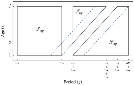
5.2.2. Age-Period Arrays. An age-period data array is rectan-gular in the age and cohort indices and given by
Iap= {(𝑖, 𝑗) : 𝑖 = 1, . . . , 𝐼, 𝑗 = 1, . . . , 𝐽} . (52)
Consequently, the cohort index𝑘 = 𝑗 − 𝑖 + 𝐼varies over𝑘 =
1, . . . , 𝐾 = 𝐼 + 𝐽 − 1. Keiding [20] refers to this Lexis diagram as the third principal set of death.
Age-period arrays are commonly used in epidemiology, in mortality analysis, and in sociology. The analysis of identification issue is largely similar to that of age-cohort arrays. However, the representation of the predictor 𝜇 in terms of𝜉differs in an intriguing way, because the third time index, the cohort𝑘, is the difference of the other two indices. The age-period-cohort model for the age-period arrays is parametrised by
𝜇𝑖𝑗= 𝛼𝑖+ 𝛽𝑗+ 𝛾𝑗−𝑖+𝐼+ 𝛿 for𝑖, 𝑗 ∈Iap. (53)
The time effect𝜃 = (𝛼1, . . . , 𝛼𝐼, 𝛽1, . . . , 𝛽𝐽, 𝛾1, . . . , 𝛾𝐾, 𝛿)now varies inΘ = R2(𝐼+𝐽). A representation of the predictor𝜇in terms of the canonical parameter𝜉is now
𝜇𝑖𝑗= 𝜇𝐼1+ (𝑖 − 𝐼) (𝜇𝐼1− 𝜇𝐼−1,1) + (𝑗 − 1) (𝜇𝐼2− 𝜇𝐼1)
+𝐼−2∑
ℓ=𝑖 𝐼−2
∑
ℎ=ℓ
Δ2𝛼 ℎ+
𝑗
∑
ℓ=3 ℓ
∑
ℎ=3
Δ2𝛽 ℎ
+𝑗−𝑖+𝐼∑
ℓ=3 ℓ
∑
ℎ=3
Δ2𝛾ℎ+2.
The representation (54) differs from that of (49) in a subtle way. The three reference points for the levels of the predictor are chosen in the corner𝑖 = 𝐼,𝑗 = 1. From this corner period and cohort indices increase, while age decreases. Hence, the age double differencesΔ2𝛼𝑖 are now cumulated backwards. This phenomenon arises because the cohort index is the difference of the principal indices of age and period, whereas for the age-cohort array the period index is the sum of the principal indices of age and cohort. The predictor is now
𝜇 = 𝑋𝜉where, withℎ(𝑡, 𝑠) =max(𝑡 − 𝑠 + 1, 0),
𝜉 = (𝜇𝐼1, 𝜇𝐼1− 𝜇𝐼−1,1, 𝜇𝐼2− 𝜇𝐼1, Δ2𝛼3, . . . , Δ2𝛼𝐼,
Δ2𝛽3, . . . , Δ2𝛽𝐽, Δ2𝛾3, . . . , Δ2𝛾𝐾), (55)
𝑋𝑖𝑗= {1, 𝑖 − 𝐼, 𝑗 − 1, ℎ (1, 𝑖) , . . . , ℎ (𝐼 − 2, 𝑖) ,
(𝑗, 3) , . . . , ℎ (𝑗, 𝐽) , ℎ (𝑗 − 𝑖 + 𝐼, 3) , . . . ,
ℎ(𝑗 − 𝑖 + 𝐼, 𝐾)}.
(56)
The identification relies onTheorem 4. It is specialised to age-period arrays as follows.
Theorem 6 (see [24, Theorem 4.1]). Let 𝜇 satisfy(53). The parameter𝜉of (55)satisfies the following:
(i)𝜉is a function of𝜃which is invariant to the group𝑔in (44);
(ii)𝜇is a function of𝜉, because of (54);
(iii)the parametrisation of𝜇by𝜉is exactly identified in that
𝜉† ̸= 𝜉‡⇒ 𝜇(𝜉†) ̸= 𝜇(𝜉‡).
The group of transformations in (44) can be specialised as
𝑔 : ( 𝛼𝑖 𝛽𝑗 𝛾𝑖−𝑖+𝐼
𝛿
) → (
𝛼𝑖+ 𝑎 + 𝑑𝑖 𝛽𝑗+ 𝑏 − 𝑑𝑗 𝛾𝑗−𝑖+𝐼+ 𝑐 + 𝑑 (𝑗 − 𝑖 + 𝐼)
𝛿 − 𝑎 − 𝑏 − 𝑐 − 𝑑𝐼 )
for𝜃 ∈ Θ =R2(𝐼+𝐽); (57)
see, for instance, Carstensen [29]. This is of the form (8) with
𝜁 = (𝑎, 𝑏, 𝑐, 𝑑)and
𝐴⊥= (1 1 ⋅ ⋅ ⋅ 1 1 1 ⋅ ⋅ ⋅ 1 1 1 ⋅ ⋅ ⋅ 1 −1−1−1
1 2 ⋅ ⋅ ⋅ 𝐼 −1 −2 ⋅ ⋅ ⋅ −𝐽 1 2 ⋅ ⋅ ⋅ 𝐾 −𝐼) . (58)
5.2.3. Period-Cohort Arrays. An age-period data arrays is rectangular in the age and cohort indices and given by
Ipc= {(𝑗, 𝑘) : 𝑗 = 1, . . . , 𝐽, 𝑘 = 1, . . . , 𝐾} . (59)
Consequently, the age index 𝑖 = 𝑗 − 𝑘 + 𝐾 varies over
𝑖 = 1, . . . , 𝐼 = 𝐽 + 𝐾 − 1. Keiding [20] refers to this Lexis diagram as the second principal set of death. Age-period arrays are commonly used in prospective cohort studies in
epidemiology and in sociology. The analysis is similar to that of age-period arrays when swapping the role of age and cohort.
The age-period-cohort model for the age-cohort arrays is parametrised by
𝜇𝑗𝑘= 𝛼𝑗−𝑘+1+ 𝛽𝑗+ 𝛾𝑘+ 𝛿 for𝑗, 𝑘 ∈Iap. (60)
The time effect𝜃 = (𝛼1, . . . , 𝛼𝐼, 𝛽1, . . . , 𝛽𝐽, 𝛾1, . . . , 𝛾𝐾, 𝛿)now varies inΘ =R2(𝐽+𝐾). A representation of the predictor𝜇in terms of the canonical parameter𝜉is now
𝜇𝑗𝑘= 𝜇1𝐾+ (𝑗 − 1) (𝜇2𝐾− 𝜇1𝐾) + (𝑘 − 𝐾) (𝜇1𝐾− 𝜇1,𝐾−1)
+𝑗−𝑘+1∑
ℓ=3 ℓ
∑
ℎ=3
Δ2𝛼ℎ+∑𝑗
ℓ=3 ℓ
∑
ℎ=3
Δ2𝛽ℎ
+𝐾−2∑
ℓ=𝑖 𝐾−2
∑
ℎ=ℓ
Δ2𝛾ℎ+2.
(61)
Thus, the canonical parameter and the design matrix are given by
𝜉 = (𝜇1𝐾, 𝜇2𝐾− 𝜇1𝐾, 𝜇1𝐾− 𝜇1,𝐾−1, Δ2𝛼3, . . . , Δ2𝛼𝐼,
Δ2𝛽3, . . . , Δ2𝛽𝐽, Δ2𝛾3, . . . , Δ2𝛾𝐾), (62)
𝑋𝑗𝑘= {1, 𝑗 − 1, 𝑘 − 𝐾, ℎ (𝑗 − 𝑘 + 1, 3) , . . . , ℎ (𝑗 − 𝑘 + 1, 𝐼) ,
ℎ(𝑗, 3), . . . , ℎ(𝑗, 𝐽), ℎ(1, 𝑘), . . . , ℎ(𝐾 − 2, 𝑘)}.
(63)
In parallel with Theorem 6 we then have the following identification result.
Theorem 7. Let𝜇satisfy(60). The parameter𝜉of(62)satisfies the following:
(i)𝜉is a function of𝜃which is invariant to the group𝑔in (44);
(ii)𝜇is a function of𝜉, because of (61);
(iii)the parametrisation of𝜇by𝜉is exactly identified in that
𝜉† ̸= 𝜉‡⇒ 𝜇(𝜉†) ̸= 𝜇(𝜉‡).
5.3. Expressing the Age-Cohort Model as a Hypothesis. It is often of interest to test the absence of the period effect. An application to analysing asbestos related mortality can be found in Miranda et al. [24].
The hypothesis is that𝛽1 = ⋅ ⋅ ⋅ = 𝛽𝐽, when expressed in terms of the time effect parameters. The restricted model is given by, with𝑘 = 𝑗 − 𝑖 + 𝐼,
𝜇ac
𝑖𝑗 = 𝛼𝑖+ 𝛾𝑗−𝑖+𝐼+ 𝛿 for 𝑖, 𝑗 ∈Iap. (64)