City, University of London Institutional Repository
Citation
:
Wang, J., Ma, Q. and Yan, S. (2016). A hybrid model for simulating rogue wavesin random seas on a large temporal and spatial scale. Journal of Computational Physics, 313, pp. 279-309. doi: 10.1016/j.jcp.2016.02.044
This is the accepted version of the paper.
This version of the publication may differ from the final published
version.
Permanent repository link:
http://openaccess.city.ac.uk/15705/Link to published version
:
http://dx.doi.org/10.1016/j.jcp.2016.02.044Copyright and reuse:
City Research Online aims to make research
outputs of City, University of London available to a wider audience.
Copyright and Moral Rights remain with the author(s) and/or copyright
holders. URLs from City Research Online may be freely distributed and
linked to.
City Research Online: http://openaccess.city.ac.uk/ [email protected]
* Corresponding author.
E-mail address: Q. [email protected]
A hybrid model for simulating rogue waves in random seas on
a large temporal and spatial scale
Jinghua Wang, Q.W. Ma*, S. Yan
School of Mathematics, Computer Science and Engineering, City University London, EC1V 0HB, UK
Abstract
A hybrid model for simulating rogue waves in random seas on a large temporal and spatial scale is proposed in this paper. It is formed by combining the derived fifth order
Enhanced Nonlinear Schrödinger Equation based on Fourier transform, the Enhanced Spectral Boundary Integral (ESBI) method and its simplified version. The numerical techniques and
algorithm for coupling three models on time scale are suggested. Using the algorithm, the switch between the three models during the computation is triggered automatically according to wave nonlinearities. Numerical tests are carried out and the results indicate that this hybrid
model could simulate rogue waves both accurately and efficiently. In some cases discussed, the hybrid model is more than 10 times faster than just using the ESBI method, and it is also
much faster than other methods reported in literature.
Keywords: Hybrid model. Rogue wave. Random wave. Large scale. FFT
1 Introduction
1.1 Background
The study of surface ocean waves has a long history [1, 2, 3, 4, 5], however, rogue waves didn’t draw extensive attentions until recent decades. The rogue waves are extraordinarily large water waves in ocean and have been recognized as great threats to the safety of offshore structures [6, 7]. It is commonly defined as the wave with maximum wave height exceeding 2
times of significant wave height (Hs) and/or the maximum wave amplitude exceeding 1.25 Hs
[8]. Their occurrence is in fact more frequent than rare [9]. The rogue waves might be caused by many factors, such as the energy focusing due to the seabed geometry, wind-wave
interaction, wave-current interaction, modulation instability, etc., which have been discussed and reviewed by researchers [9, 10].
The most distinguished feature of rogue wave is its transience, which means that it can happen and disappear very rapidly [9]. Due to that reason, it cannot be modeled by using
steady wave theories, e.g., Stokes waves [4], cnoidal waves [11] or solitary wave [12], which describe such waves with permanent profiles not evolving in time. Furthermore, due to the
rapid appearance of rogue waves and the persistently changing sea state, the statistical stationarity condition also breaks down [9]. Therefore, studies need be carried out in time
domain to explore the physics of rogue waves.
2
order wave theories significantly underestimate the rogue wave dynamics, thus third or higher order or fully nonlinear theories are required [16], which also has been confirmed by
numerical simulations in [17, 18]. In addition, the nonlinearities of rogue waves are so strong that sometimes breaking occurs in many occasions. In order to deal with these cases, the Navier-Stokes (NS) equations may be numerically solved, as has been done by, e.g., Harlow
and Welch [19] and Hirt and Nichols [20]. However, this class of methods is so inefficient that it is impossible to be employed for a large scale simulation even with the very powerful
computer available today.
On top of that, the studies on rogue waves have already been carried out extensively on
the local scale, such as rogue wave interaction with wind [21, 22], current [23, 24] and structures [25, 26], etc. The work significantly contributed to our understanding of the local
effects of rogue waves over a short window of time. However, the formation of rogue waves in random seas is not fully explained by using the knowledge of the local effects [9]. To fully
understand the formation for rogues, simulations of wave fields in large and long time scale with sufficient nonlinear effects are needed as indicated by [27].
The statistical studies have suggested that the rogue waves usually have exceedance
probabilities ranging from 10-3 to 10-5 [10]. Unquestionably, it may take long duration to
observe an occurrence of the rogue wave directly from random sea simulation either
physically or numerically. For example, within the range of real observation, one may need to record 103 ~ 105 individual waves to collect reliable statistics, e.g. 3000 waves based on
Rayleigh distribution [9]. Most importantly, in such a way, the occurrence of the rogue waves is random and unpredictable. It may appear after a sufficient long-time evolution due to
nonlinearity, thus the duration of the numerical simulation must be long enough, e.g., covering the life span of one random sea state. Duration shorter than this may not well
represent the evolution of random seas. Since the real sea states averagely last for 3 hours [28], and a typical peak period in North Sea [29, 30], the duration of the simulation may
need to last as long as approximately .
In addition, traditional statistical model only looks at the surface time history at a fixed location. While rogue waves can occur at arbitrary position during the nonlinear evolution, so
that regional statistics must be considered [31]. According to Forristall’s study on the air gap under the deck of a platform [32], the maximum crest height in the whole working area
( ) is almost 20% higher than the one expected at a single point. This further addresses the importance for developing a statistical model describing wave probability over
a specific area, instead of just looking at a fixed location [9]. However, very few studies on regional statistics of rogue waves have been carried out so far, although researchers are aware
that higher crests appear in radar images [32]. Meanwhile, instead of directly using such statistical model, random seas may be simulated numerically so that the free surface can be
obtained at every time step, which can later be used for regional statistics. To do so, the domain should be large enough to account for the possible locations where rogue waves may occur as the location of rogue waves are unpredictable. For long-crest waves, i.e., in 2D
3
waves in a large temporal and spatial scale. A brief review on them will be given in the following subsections.
1.2 Numerical models for large scale simulations
Phase-averaged or the so called third generation wind wave models, such as WAM, SWAN, WAVEWATCH etc., have long been suggested and widely adopted in engineering and
applied sciences. However, only the statistic features of the waves could be obtained, such as the peak frequency, significant wave height and so on. The space-time information of the
specific wave dynamics is lost by using them, which however is very important for considering the dynamics of rogue waves for different purposes. Thus, phase-resolved models
have been sought after. Among them, numerical models based on the NS equation are not computationally economical for large scale simulations as pointed out above and such
applications in literatures are rare. The potential theory assumes that the fluid is inviscous and irrotational, which makes numerical simulations much faster. Therefore, we will only consider
potential models in the present study to simulate non-breaking waves, and so the review below will be focused on the work related to using potential models.
1.2.1 Weakly nonlinear models
The simplified mathematical models, such as the Boussinesq, KdV, and Schrödinger equations have been widely used to study weakly nonlinear waves. The Boussinesq equation
[12] and KdV equation [11] were derived by assuming small steepness and water depth to study shallow water waves. Both the equations are obtained by assuming the Ursell number
[33]. Thus they are mainly used for studying weakly nonlinear waves in shallow water situations. Although improved models which could be used in deep water are
suggested, such as the higher order Boussinesq equation by Wei et al. [34] and. Madsen et al [35], as well as multi-layered Boussinesq model by Lynett and Liu [36], they are relatively
computational expensive so that are hardly used in large scale simulations. Nevertheless, both the KdV and Boussinesq equations are only accurate when used to simulate waves in shallow
and finite water depth, so that they will not be further discussed in this paper. A detailed review about the KdV and Boussinesq equation could be found in [37].
The nonlinear Schrödinger equation (NLSE) is another tool to study the dynamics of the
gravity water waves in deep and finite water depth. Thethird order weakly nonlinear equation was first derived from the Zakharov equation [38], which is referred as the cubic NLSE
(shortened as CNLSE) in this paper. Subsequently, Benny and Roskes [39], Hasimoo and Ono [40], Davey and Stewartson [41] also came up with the similar equations by using
perturbation method. Based on the previous studies, Dysthe [42] extended this theory to the fourth order for narrow bandwidth waves and proposed what is referred to the Dysthe
equation. Trulsen and Dysthe [43] further extended the work and derived an equation for broader bandwidth waves. Later, Trulsen et al [44] corrected the linear terms to the exact
4
[42], which indicates that the Dysthe equation is a special case of the Zakharov equation. Debsarma and Das [46] used the same technique and obtained a fifth order equation called the
Higher Order Dysthe Equation in terms of Hilbert transform. Similarly, by introducing Trulsen et al.’s approach [44], the linear operation of this equation could be enhanced and we
refer it as the fifth order Enhanced Nonlinear Schrödinger Equation based on Hilbert
transform (shortened as ENLSE-5H) in this paper.
Applications of Schrödinger type equations in large scale simulations are extensive.
Dysthe et al. [47] investigated free surface evolution by directly simulating random waves
based on the Dysthe equation in a domain covering 100 100 peak wave lengths for 150 peak periods. Onorato et al. [48] brought the effects of current into the CNLSE and showed that rogue waves can be generated naturally when a stable wave train enters a region of an
opposing current flow based on a numerical simulation in a domain of 60 peak wave lengths lasting for 60 peak periods. In addition, Shemer et al. [49] studied the probability of rogue
waves in random wave simulations based on both the CNLSE and the Dysthe equation in a domain of 77 peak wave lengths during 100 peak periods. More studies can also be found in [50, 51].
1.2.2 Fully nonlinear models
Besides, studies of rogue waves have also been carried out by using the fully nonlinear
potential theory. Some papers employed Boundary Element Method (BEM) [52, 53], and others used Finite Element Method (FEM) [54, 55] or Quasi Arbitrary Lagrangian-Eulerian
Finite Element Method (QALE-FEM) [26, 56]. Some of these methods can simulate waves with overturning (e.g. [53, 56]) but they are relatively expensive, so they have not been
applied to modelling wave in vary large scale so far. Another category of nonlinear potential methods is based on the FFT. One of them is the Higher-Order Spectral (HOS) method
proposed by West et al. [57], and subsequently by Dommermuth and Yue [58] to simulate propagating waves. This method applied the Taylor expansion of the velocity potential on the
free surface with respect to vertical coordinate. It is accurate and efficient when the waves to be studied are not very steep ( ) [58]. Nicholls [59] suggested a numerical model called Spectral Continuation method to study the traveling water wave problems. The
Dirichlet-Neumann operator is approximated by a limited Taylor series. Due to the fact that evaluating the higher order terms is highly recursive and impractical, they chose to use the
expansions to thefifth order in practice. As a consequence, this method is incapable to capture the higher order nonlinearities and only accurate when the nonlinearities are weak. Clamond
and Grue [60] suggested another method combing boundary integral equations and FFT technique in two and three dimensions. The formulations for 3D situation was later
implemented and numerically tested by Fructus et al. [61] and Grue [62], named as the Spectral Boundary Integral (SBI) method. This method is recently improved and enhanced by
Wang and Ma [63] in three aspects including provision of new techniques for anti-aliasing and de-singularization, and a new algorithm for automatically including or excluding integral terms involved in the method. It has been observed that the new technique can help the
5
The method presented by Wang and Ma [63] with the new techniques will be referred as to Enhanced Spectral Boundary Integral (ESBI) method in this paper for convenience.
The FFT based fully nonlinear methods have been successfully applied in large scale simulations. Clamond et al. [64] simulated the evolution of wave groups by using the SBI method in a 2D NWT covering 128 peak wave lengths up to 2000 peak periods. Ducrozet et
al. [29] had investigated the occurrence of rogue waves in 2D and 3D large open seas of
peak wave lengths for 250 peak periods by direct simulation of random waves using HOS method. Xiao et al. [65] also studied the dynamics of rogue waves in 3D NWT covering
peak wave lengths which lasts for 150 peak periods based on HOS to account for the directional spreading effects.
1.3 Issues to be addressed
As indicated above, the literature reveals that rogue waves need to be modelled in a large temporal and spatial scale with full consideration of nonlinearity. In addition, a large number
of parameter studies are required to quantify the behaviors of rogue waves as shown Xiao et al. [65] and in engineering design. This inheritably demands the modelling methods to be efficient. Although versatile versions of NLSE have been suggested and are computationally
efficient, they are only accurate when waves are moderate. Henderson et al. [66] simulated traveling waves based on the CNLSE and fully nonlinear Higher-Order BEM, and concluded
that there was good agreement between the results of these two models only for waves with
small steepness ( ). Clamond et al. [64] investigated the evolution of the envelope soliton with an initial steepness of using the ENLSE-4 and their fully nonlinear approach separately.Through comparing the free surface profiles, they concluded
that the former was only valid for a limited period at the beginning of the simulation before rogue waves are formed, and indicated that the ENLSE-4 became inaccurate when wave
steepness evolved to be .Slunyaev et al. [67] have compared the analytical solution of the CNLSE with the numerical results of the Dysthe equation and the fully nonlinear Euler
equations for simulating rogue waves. They concluded that the CNLSE was not accurate for waves with initial steepness .
On the other hand, the fully nonlinear models are more accurate than the weakly
nonlinear models for dealing with strong nonlinear waves, one should note that they are relatively more computationally expensive. It was reported, for example, by Ducrozet et al.
[29] that the simulation of a 3D random sea covering peak wave lengths and propagating for 250 peak wave periods costs 10 CPU days on a 3 GHz-Xeon single processor
PC by using the fifth order High-order Spectral method! It is far longer than a sea state ( ). That indicates that the existing fully nonlinear models are not sufficiently efficient
for a large scale simulation and for use in design where a large number of parameter studies may be necessary.
In summary, there is currently a lack of numerical methods which can model rogue waves in a large scale with full nonlinearity and with sufficient efficiency. In this paper, we will propose a new hybrid model coupling the models with different levels of approximations
6
models are used; only when necessary, the fully nonlinear but less efficient models are employed. In this way, one can achieve higher efficiency without loss of accuracy. The ESBI
described in [63] will be selected as the fully nonlinear model. The ENLSE-5H suggested by Debsarma and Das [46], will be used as the simplified and efficient model but will be reformulated to overcome some of its drawbacks. As well known, the ENLSE is accurate only
with relatively narrow bandwidth waves, but may not be accurate for broad bandwidth waves even their steepness is not very large. A proper alternation is needed to replace the ENLSE for
modelling waves of broad bandwidth with moderate steepness. This will be obtained by a reduced form of the ESBI. The relevant techniques for coupling the models will be detailed in
the following sections.
2 Mathematical formulations
2.1 The Spectral Boundary Integral Method
This method has been suggested by Clamond and Grue [60], Fructus et al. [61] and Grue
[62], and improved by Wang and Ma [63]. So details will not be given here. However the summary of main equations is just presented for completeness. Based on the potential theory, the governing equation together with all boundary conditions are given as
(1)
(2)
(3)
(4)
where is the Laplacian and is the horizontal gradient
operator, and is the elevation of the free surface, is the velocity potential. Among the
variables in the equations above, , and have been non-dimensionalized by
multiplying , by multiplying and by multiplying , where
is the representative circular frequency and is the gravity acceleration.
In order to derive the equations for numerical simulation, the Fourier transform and the inverse transform are employed and defined as
(5)
(6)
7
The boundary conditions on the free surface could be reformulated as
(7)
(8)
after introducing and the velocity potential at free surface . This is referred as the Dirichlet to Neumann operation. Applying Fourier transform to both the boundary conditions leading to the skew-symmetric prognostic equation
(9)
where
, , (10)
and the circular frequency , wave number . Then the solution
is given as
(11)
where
(12)
On the other hand, the boundary integral of Green’s theorem based on Eq. (1) follows as
(13)
where S is the area of the instantaneous free surface, the variables with the prime indicate those at source point , the variables without the prime are those at field point ,
and , denotes the segment of .
Using , the above integral can be written as
(14)
8
(15)
The velocity can be split into four parts, i.e., . Each part is given by
(16)
(17)
(18)
(19)
where and could be estimated directly by applying the Fourier and its inverse
transforms. Fructus et al. [61] has rewritten the kernel of , and the dominant part could be expanded into thethird order convolutions, say
(20)
The calculation of the convolutions is very fast owing to the algorithm of FFT. Otherwise, the remaining integration part of and the whole expression of are estimated through
numerical integration, which is the most time consuming part of the numerical method. In addition, the numerical integration is estimated at nodes and shifted back to regular points through Fourier interpolation in order to avoid explicit singularity for
calculating the integrand in [61]. It is found that the resolution needs to be well refined in order to obtain accurate results by using this method. Grue [62] made one step further,
expanded the kernels of and and wrote the dominant parts into the convolutions up to
thesixth andseventh order respectively. Both the remaining integration parts of and are neglected. The numerical scheme is significantly accelerated due to the most time consuming parts are excluded. However, it is based on the assumption that the gradient
parameter . If the condition is not met, such as the cases where the wave free surface is quite steep even in a local area, the integration parts can be important to the accuracy of
estimating and and could not be neglected.
9
computational efficiency of this numerical model have been proposed. Firstly, a new numerical de-singularity technique was introduced. It is found that to reach the same level of
accuracy, one could use much less points if the new method is applied. The second contribution of that paper was to propose a new technique to deal with anti-aliasing problem associated with FFT/IFFT. The other contribution they made was to reformulate the equation
for and as
(21)
(22)
During their simulation, the gradient of wave surface is monitored. When the waves
satisfy a condition that they are moderate or their gradient is small, the velocity components will be evaluated through only estimating convolutions up to theseventh order with the
integration parts neglected. The integration parts are estimated only when the condition is not met. For regular waves, the condition is , where can be taken as 0.5. For
random waves, the condition is , where is theeighth order
convolution part. With the three new techniques, the method becomes much faster. It has been observed to be more than 35 time faster than the method without the techniques in some cases. The method presented by Wang and Ma [63] will be referred to as Enhanced Spectral
Boundary Integral (ESBI) method in this paper for convenience.
Built on that paper, another computational efficient method may be formed, in which
only thethird order convolution terms, neglecting the integration terms in the vertical velocity,
i.e., are considered. The difference between this approximate approach and the ESBI lies in the vertical velocity estimation. All others, including the prognostic equation and full nonlinear free surface conditions, are the same as the ESBI. It is expected
that this approximate approach will be as accurate as the ESBI when the waves are not strongly nonlinear. This approximate approach will be referred as the Quasi Spectral Boundary Integral (QSBI) method in this paper for convenience. Both the QSBI and ESBI
methods are solved by using embedded fifth order Runge-Kutta method with adaptive time step. The details of the numerical scheme could be found in [63]. The QSBI will be formed as
a part of the hybrid method developed in this paper.
2.2 The ENLSE based on FFT
In this section, the formulations of the ENLSEs will be presented. In the first subsection, the various forms of existing ENLSEs are outlined. The second subsection then explains the
ENLSE based on FFT, newly proposed in this paper. Details are given below.
2.2.1 Existing ENLSEs
10
potential could be written in the form of the summation of harmonics by introducing the concept of envelope
(23)
(24)
where and are complex envelops of the first harmonic of surface elevation and velocity
potential respectively, and are the harmonic coefficients, and are real functions representing the mean surface deflection and mean flow, is the complex
conjugate, and with being the main direction of wave propagation. , and have been non-dimensionalized by multiplying , while , and
non-dimensionalized by multiplying , similar to what have been done for the variables
in Eqs. (1)-(4). Subjected to the assumption that steepness and spectrum width is of order , one can introduce the slow modulation variables , and , and assume and are slowly modulated by such variables. Using the perturbation
approach to thefourth order , one can obtain the Dysthe equation [42, 45], which is in terms of . One can also obtain the Dysthe equation of the second kind [68] in term of wave
envelope , which is employed in this paper:
(25)
(26)
(27)
(28)
where the superscript denotes its complex conjugate. The order (I) of the equation is defined in the way that
,
, and (29)
Trulsen et al. [44] later pointed out that the linear operators could be replaced by the
exact linear solution, and proposed the following form
11
where and is the peak wave number. Note that we have
assumed that the mean wave direction points to the positive x-axis. The linear terms on the
left hand side now become the exact representation of linear propagation and no longer subject to the narrow spectrum assumption. The nonlinear terms on the right hand remain the same. The method based on Eq. (30) is named as ENLSE-4 in this paper for convenience. The
term needs to be determined before the equations can be solved numerically, which is given by Eq. (A. 8) in Appendix-I. Substituting Eq. (A. 8) into Eq. (30), we have the other
form of the ENLSE-4
(31)
where
(32)
(33)
and is the Fourier transform defined by Eq. (5) and (6). Eq.(31) is equivalent to the
equation of first kind in terms of derived by Clamond et al. [64], and is easy to be solved
numerically if the initial condition is given.
Zakharov [38] had pointed out that the CNLSE could be derived from the Zakharov equation with narrow spectrum assumption. Later, Stiassinie [45] found that the Dysthe
equation could also be derived from Zakharov equation by expanding the nonlinear terms to the specific order. Based on the same idea, Dabsarma and Das [46] made one step further and
obtained the Higher Order Dysthe equation in terms of the Hilbert transform. Specifically, they gave the following equations
(34)
where the nonlinear part
(35)
12
and the Hilbert transform is
(37)
(38)
For convenience, this formulation is named as ENLSE-5H.
2.2.2 The ENLSE-5F
In order to estimate the Hilbert transform, i.e., the Cauchy integral, involved in , numerical integration should be used. The difficulties with performing the numerical
integration for these Cauchy integrals exist in two aspects. Firstly, the range of the integration
is from to , although it could be optimized to a limited range, a large number of numerical tests may need to be carried out in order to determine this range and the tests may be needed for different cases as the range may depend on the specific value of envelope.
Secondly, the integrals are weakly singular at and so they require de-singular technique. Although the techniques can be developed, they need extra computational effort. In order to eliminate the difficulties, we suggest an equivalent formulation by introducing the
following substitution (refer to Appendix-II)
(39)
(40)
Using the definitions, Eqs. (34) to (36) are then replaced by
(41)
where
13
The new form (Eq.(41) and (42)) is referred as the fifth order Enhanced Nonlinear Schrödinger Equation based on Fourier transform, shortened as ENLSE-5F.
Through comparing and , it is found that the difference between the ENLSE-5H and ENLSE-5F is that the terms involving the Hilbert transform are now replaced with these in terms of the Fourier transform. The benefit by this substitution is that it is much easier to
perform the Fourier transform than the Hilbert transform. In the ENLSE-5F, there are no difficulties described above associated with ENLSE-5H. Another benefit of using the
ENLSE-5F is that it is also solved by FFT technique, same as for the ESBI and QSBI methods. If the ENLSE-5H would be coupled with them, extra FFT analysis must be
performed after numerically estimating the Hilbert transform, which needs extra computational time. Nevertheless, it requires performing FFT twice for each corresponding
term in Eq. (42), so that further investigations are needed in order to compare the
computational efficiency with estimating by using numerical integration. Furthermore, the periodical boundary condition needs to be imposed in the new formulation. However, following other studies on large scale random sea simulations [29, 31, 50, 65], the random sea states are usually reconstructed by assuming periodical boundary condition.
In addition, comparing the nonlinear part of the ENLSE-4, i.e., Eq. (32) with that of
ENLSE-5F, i.e., (42), it is found that, apart from and , there are
also and the rest parts in terms of the Fourier transform of order in Eq. (42). That means that the nonlinear effects in the ENLSE-5F are one order higher than the ENLSE-4.
3 Numerical techniques for coupling the ENLSE-5F, QSBI and ESBI
Table 1
Short summary of the three models
ENLSE-5F QSBI ESBI
Efficiency Super-fast. Most efficient among the
three models.
Very fast. Efficiency between the ENLSE-5F
and ESBI.
Fast. Least efficient among the three models
Accuracy Accurate for small steepness and narrow
spectrum waves. Least accurate among the
three models
Accurate for small and mild steepness waves.
Accuracy between the ENLSE-5F and ESBI
Accurate for small, mild and large steepness
waves. Most accurate among the three models
Three methods (ESBI, QSBI and ENLSE-5F) described above are summarized in Table 1. The ESBI is the most accurate among the three as it is a fully nonlinear model without
ignoring any necessary terms. Although QSBI only gives the solution of vertical velocity to the third order, the boundary conditions and governing equations remain to be fully nonlinear.
There will not be significant difference between the ESBI and QSBI when the wave steepness is not high. The ENLSE-5F like other NLSE models is derived from simplified boundary
[image:14.595.84.510.487.638.2]14
ENLSE-5F is the least accurate model among all. On the other hand, the ENLSE-5F is the most efficient model. Due to the complexities in solving for the vertical velocity, the QSBI
costs more computational efforts than the ENLSE-5F. Furthermore, the involvements of higher order nonlinear parts in solving for the vertical velocity make the ESBI less efficient than the QSBI. In terms of accuracy there is a relation: ESBI > QSBI > ENLSE-5F while
ENLSE-5F > QSBI > ESBI in terms of efficiency, where ‘>’ means superior. Based on this, a hybrid method will be formed using the three methods, which is both accurate and efficient,
making use of the advantages of the three methods. For this purpose, the three methods (ESBI, QSBI and ENLSE-5F) should be alternatively and automatically employed according to the
instantaneous wave information. That is, the simulation of the hybrid method will involve the switching from one model to another. To do so, the following challenges need to be tackled.
a) The conditions need to be found out to determine which model is employed during simulation and when switching to others. This will be discussed in Section 3.2.
b) To employ the three models alternatively, exchanging data from the ENLSE-5F to the QSBI and ESBI is necessary, i.e., the outputs of the ENLSE-5F need to be transformed to the forms accepted by the QSBI and ESBI as their input. The solution
obtained from the ENLSE-5F at each time step is the free surface envelope . To use them as the input for the QSBI and ESBI, the expressions for the free surface
elevation and velocity potential in terms of needs to be derived. This will be discussed in Subsection 3.1.1.
c) On the other hand, in order to exchange data from the QSBI and ESBI to the ENLSE-5F, their outputs need to be transformed to the forms of the input for the
ENLSE-5F, which will be resolved in subsection 3.1.2.
3.1 Relationship between and
3.1.1 Transformation from to and
As can be seen from equations given in previous sections, the solution of the ENLSE-5F
is given in terms of envelop , but and are required to start the QSBI or ESBI. Therefore, there is a need to transform to and when switching from the ENLSE-5F simulation to the QSBI or ESBI simulations. According to Eq. (23) and (24), we just need to
estimate the harmonic coefficients , , , , , and the term of . As shown in Appendix-III, they can be determined by using Eq.(A. 21), (A. 22), (A. 30), (A. 31), (A. 19)
and (A. 24) respectively.
It is worth of noting that (A. 30) is different from Hogan’s formulation [69], i.e.,
, which only considers the approximate linear evolution of and nonlinear effects are neglected. In contrast, (A. 30) involves the nonlinear effects up to the
15
3.1.2 Transformation from to
When switching the modelling from the QSBI or ESBI simulations to the ENLSE-5F simulations, one needs to obtain the expression for envelop used for the input to the latter. That means that the spatial solution of the free surface elevation from the QSBI or ESBI
needs to be transformed to the envelop . In order to do so, we rewrite Eq.(23) as
(43)
where
(44)
are the 1st, 2nd and 3rd harmonics of the free surface elevation, respectively. The relationship
between and is established by using (A. 38) in Appendix-IV. In addition, , and
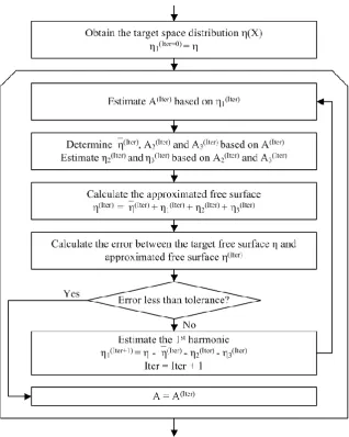
could be estimated with the help of Eq.(A. 21), (A. 22) and (A. 24). However, it is the value of that is given from the solution of the QSBI or ESBI instead of , , and . To overcome this dilemma, iterations are carried out for obtaining the solution from ,
which is graphically illustrated in Fig. 1. It is noted that and are in the same order, which are normally much larger than , and , and so the iterative procedure starts
16
Fig. 1. Flow chart of estimating the envelope by iterations
The error represents the difference between the target surface and the approximated surface is given as
(45)
We have found that is enough to give very precise results.
3.2 Methodology for combining three methods
In order to form a hybrid method, the three methods ─ ENLSE-5F, QSBI and ESBI need to be combined together. To do so, the key thing is the conditions under which the simulation
is switched from one to another. For this purpose, we introduce four conditions:
a) Condition 1: , and
[image:17.595.149.468.74.473.2]17
c) Condition 3: d) Condition 4: where
(46)
(47)
The basic idea of the four conditions aforementioned is to measure the intensity of the
nonlinearities, i.e., the stronger the waves are, the larger and are. The first two conditions are used to control the switch between the ENLSE-5F and QSBI. If the waves keep
growing, and finally the steepness is larger than the initial steepness and , Condition 1 is met and the waves are no longer weakly nonlinear, which means actions should
be taken to replace the ENLSE-5F by using the QSBI. Vice versa, if Condition 2 is met, the ENLSE-5F will be recovered. Similarly, the last two conditions are used to control the switch
between the QSBI and ESBI. If , the nonlinearities become so strong that the QSBI should be replaced with the ESBI, and vice versa.
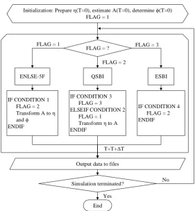
With the four conditions and the formulas for the errors above, the flow chart for the
hybrid method is given in Fig. 2. It shows that the procedure starts with ENLSE-5F for waves with small steepness; when Condition 1 is met (the wave being steep enough), FLAG will be
assigned to be 2 and so the process will be switched to QSBI in the next time step; after the waves become steeper and so Condition 3 is met, the process will be switched to ESBI in the
next time step. During the simulation, if the waves become less steep (or Condition 4 is met), FLAG will be assigned to be 2 from the ESBI and so the process will be switched back to
QSBI, then may be to ENLSE-5F if Condition 2 is met. As can be understood, the switch is always through QSBI and there is no direct switch between the ENLSE-5F and the ESBI. It is
noted that the process can start from any one of the three methods, as long as the initial value of FLAG is assigned properly. For example, if one knows that the wave spectrum is not narrow-banded and/or the wave steepness is quite large, the initial value of FLAG may be
given as 3 and so the process will start from ESBI. Of course, the representation of the initial condition will be different if the starting method is different. Actually, the initial condition is
usually given in terms of the free surface elevation and the velocity potential on the free surface as shown in [63], which can be employed directly to start QSBI or ESBI. For start
with ENLSE-5F, the initial condition information in terms of the free surface elevation and the velocity potential needs to be transformed to the wave envelope in the similar way to that
18
Initialization: Prepare η(T=0), estimate A(T=0), determine ϕ(T=0) FLAG = 1
Output data to files Simulation terminated?
End
No T=T+ΔT
Yes
ENLSE-5F QSBI ESBI FLAG = 1
FLAG = 2
FLAG = 3 FLAG = ?
IF CONDITION 1 FLAG = 2 Transform A to η and ϕ
ENDIF
IF CONDITION 3 FLAG = 3 ELSEIF CONDITION 2 FLAG = 1 Transform η to A ENDIF
IF CONDITION 4 FLAG = 2 ENDIF
Fig. 2. Flow chart for the new hybrid method
3.3 Effects of and by numerical simulations
In order to control the switch between the three models and guarantee the final results are acceptable, proper values for and need to be specified. Thus in this section we
will discuss how the values for and are determined. For this purpose, numerical simulations of random waves in a two-dimensional domain of and duration of
will be performed by using the ENLSE-5F, QSBI and ESBI separately.
Two most frequently used spectra, JONSWAP and Wallops, will be considered. As well known, the JONSWAP spectrum is proposed for developing sea states while the Wallops
spectrum is more suitable for fully developed and decaying sea states [70]. The JONSWAP spectrum in terms of the wave number in dimensionless form is given as [28]
(48)
where the wave number has been non-dimensionalized by dividing the peak wave number
, the significant wave height by multiplying , by multiplying ,
, is
the peak enhancement factor and . The peak
[image:19.595.160.442.71.376.2]19
the spectrum is.
Meanwhile, the Wallops spectrum is reformulated by Goda [71] and its dimensionless
form is
(49)
where and
is the width parameter. The spectrum becomes narrower when increases.
Different combinations of the significant wave height and width parameter are tested based on both the JONSWAP and Wallops spectrum, in order to find proper resolution and
tolerance for time marching. The domain covers 128 peak wave lengths and is resolved into 8192 points. The spectrum is discretized by using interval ( is the domain
length), and the cut-off wave number . According to Goda [71], a cut-off frequency chosen as the 1.5 to 2.0 times the peak frequency, is enough for engineering purpose, which is
equivalent to the cut-off wave number , and is covered by that we have suggested. The errors of wave elevations will be estimated by
(50)
where is obtained by using a specific numerical model, and is the reference solution of wave elevations, which may be analytical solution or evaluated by using a relatively more accurate method.
3.3.1 Investigation on effects of
Firstly, we carry out numerical simulations based on both JONSWAP and Wallops
spectrum with different significant wave heights and spectrum width parameters spanning in
the practical range in order to find a proper value for . Because this parameter only controls the switch between the QSBI and the ESBI, and are given during the initialization in the process described in Fig. 2 in all the cases for testing effects of
.
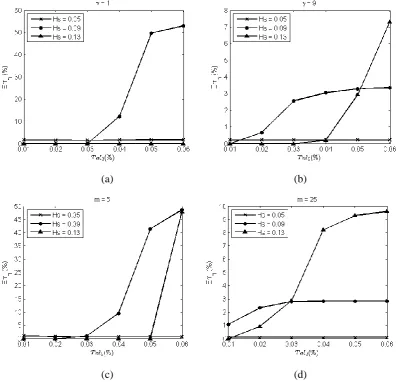
The simulations are carried out to in a two-dimensional domain of for random waves. The errors in the wave elevation are estimated by Eq. (50), in which is the free surface at the end of the simulation obtained by only using the ESBI model and is that
obtained by using the hybrid model with different values of specified. Some results are presented in Fig. 3, in which only the cases of narrowest and widest bandwidth are shown. From this figure, one can see that the trend of the error in wave elevations is very similar for
the cases with different spectra, different significant wave heights and spectrum widths. It is
20
According to tests by Wang and Ma [63], the wave elevations become invisibly different if their error estimated by Eq. (50) is less than 5%. Based on this and also other tests when preparing this paper, 5% is acceptable. Nevertheless, to be conserved and
considering that the ENLSE-5F has not been involved yet, we may accept the error ( ) of
the hybrid model to be not larger than 3% from the point of view of accuracy. On the other
hand, we also hope that the value of is as large as possible. That is because the larger
the value of is, the longer the QSBI is involved and so more computational time it saves. By examining all the curves in Fig. 3, one may find that the hybrid model with
leads to the error ( ) of less than 3% in all the cases with with different
spectra, different significant wave heights and spectrum widths. Therefore, generally,
will be adopted for controlling the switch between QSBI and ESBI.
(a) (b)
[image:21.595.93.492.293.675.2](c) (d)
Fig. 3. against . (a)(b) are based on JONSWAP spectrum and (c)(d) on Wallops
21
3.3.2 Investigation on effects of
By using , the numerical tests are carried out for the same cases again in order to find the appropriate tolerance of to control the switch between the ENLSE-5F and the QSBI. In these tests, all three models are involved in calculating the cases with
different values of specified.
The results for the error ( are shown in Fig. 4. Again, it is found that the trend of
the error in wave elevations is very similar for the cases with different parameters, and that
for a fixed and spectrum width, the error grows when increases.
As all three models are involved in these tests, 5% may be considered to be
acceptable in terms of accuracy and efficiency. By examining Fig. 4, one may find that the
condition of 5% can be satisfied if for all the cases. Therefore,
for can be used for controlling the exchange between the ENLSE-5F and QSBI.
(a) (b)
[image:22.595.93.492.340.722.2](c) (d)
22
spectrum
It is worth of noting that the tolerance and are obtained
based on large numbers of two dimensional (2D) simulations. However, it can be applied to three dimensional (3D) simulations as Eq. (46) and (47) can still be used. Next, numerical
tests will be carried out to validate the hybrid model for both 2D and 3D simulations by using the tolerances obtained in this section for switching between models.
3.4 Validation
In order to validate the present model for larger domain and longer simulations, we compare the results of the hybrid model with the results in [64]. The free surfaces at several
time steps obtained by this hybrid method and that in [64] are shown in Fig. 5. The difference between them is almost invisible, with its value at the maximum free surface being about
3.02% occurring at the end of the simulation. The comparison again indicates that the profiles by using the present method and the fully nonlinear method described in [64] are consistent.
In addition, the switch between the models is shown in Fig. 6. It is found that after the first extreme wave event, the maximum free surface elevation never drops below the initial status,
so that the ENLSE-5F is not involved again in the simulation after the first 100 periods. The rest of the simulation is completed by the switch between the QSBI and ESBI models. Nevertheless, the about 40% CPU time is saved in this case compared to that using the ESBI
model alone.
0 20 40 60 80 100 120
-0.2 0 0.2
T/T0 = 0
X/L0
0 20 40 60 80 100 120
-0.2 0 0.2
T/T0 = 410
X/L0
0 20 40 60 80 100 120
-0.2 0 0.2
T/T0 = 1500
X/L0
[image:23.595.122.468.437.722.2]
23
Fig. 6. The exchange between the models. Solid line represents the values of
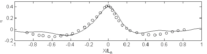
Moreover, in order to validate the hybrid model for three dimensional (3D) problems, the numerical tests for directional focusing wave described by Bateman et al. [72] is repeated
here with the same setups. A focusing wave of steepness as in [73] is generated at the center of the domain, and the profiles of the free surface along at the
focusing time for both the hybrid model and results in [72] are shown in Fig. 7. The error of the maximum surface elevation is about 2.02%, which means that the hybrid model successfully captured the occurrence of the focusing wave in the 3D case.
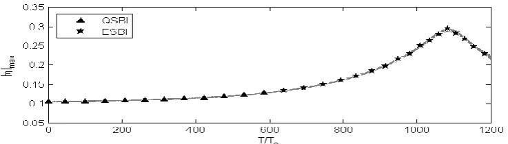
In order to show the effectiveness of the numerical technique for controlling the switch between models, the maximum free surface elevation against time is shown in Fig. 8 with
indicators of each model used at that instant. It is found that the ENLSE-5F is only involved in the first 1.5 peak periods, while the majority of the simulation is run by QSBI and ESBI.
However, it shows that the hybrid model successfully switched from the ENLSE-5F, to QSBI and then ESBI, when the maximum surface becomes larger and larger. This case with the
parameters in Section 3.3 demonstrates that the hybrid model is also suitable for 3D wave problems.
[image:24.595.119.475.533.627.2]24
Fig. 8. The exchange between the models (solid line represents the values of )
In addition, a simulation of the crescent wave pattern is also carried out in order to
further validate the hybrid model for 3D cases. The test by Fructus et al. [74] is repeated here with the same setups. The following quantity is introduced to measure the ratio of the
amplitude of component over the initial Stokes wave amplitude.
(51)
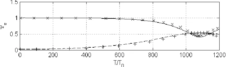
The results are presented in Fig. 9 for the components of peak wave component
and perturbation component . It shows that the results obtained by using the hybrid model is highly correlated with that obtained by using the method in [74] in this 3D case, which again confirms that the tolerance values obtained by using the 2D cases are
suitable for the 3D cases. Similar to Fig. 6, the switch between the models is shown in Fig. 10, where it is found that the ENLSE-5F is not involved and only the QSBI and ESBI are used
during the simulation for this case. And it shows that the hybrid model successfully switched from the QSBI to ESBI when the maximum wave steepness became large, which further confirms that the hybrid model can be used for simulating waves in three dimensions.
Fig. 9. Evolution of perturbation components and peak wave components: ‘—’
by using hybrid model; ‘--’ by using hybrid model; ‘x’ by
[image:25.595.112.479.552.661.2]25
Fig. 10. The exchange between the models (solid line represents the values of )
4 Discussions on the overall performance of the hybrid model
In this section, more numerical examples will be tested on the new hybrid model with
and , which are determined in Section 3.3.
We introduce the CPU time ratio that is the CPU time of the ESBI divided by that of the hybrid model. All the simulations are implemented by using a single core on the same
workstation equipped with the Intel Xeon E5-2630 v2 (Intel Corporation, Santa Clara, CA, USA) of 2.6GHz processor. Pre-tests have been carried out based on the JONSWAP spectrum
with , , and it takes the ESBI 10638s ~ 3h, the QSBI 5404s ~ 1.5h (about a half of CPU time for the ESBI), and the ENLSE-5F only 734s ~ 12min (only 7% of CPU time
for the ESBI), to finish one sea state simulation ( ) covering a two dimensional domain of 128 domain by a resolution of per independently.
Although the main purpose to develop the efficient hybrid method is for simulating the
evolution of random seas with rogues wave occurrence, our simulations in this section will be mainly focused on the cases with tailored rogue waves embedded in random background for
testing the performance of the new hybrid method and its applicability in various scenarios. That is because real rogue waves are unpredictable and could happen at arbitrary time and
location, and so directly testing on them may not be able to check the performance of the new hybrid in various scenarios. The technique of embedding rogues waves in random background
is commonly used in experiments. Different methods for embedding rogue waves in random background are suggested in literature. In order to constrain the occurrence of a rogue wave in a limited space during a predictable timeframe, Taylor, et al. [73] proposed a Constrained
NewWave theory. Clauss and Steinhagen [75] has adopted a Sequential Quadratic Programming method to optimize the location and time instance of the maximum crest in
space and time domain respectively so that an expected asymmetric wave profile is created. Kim [76] suggested a method to deform the largest crest wave by time and crest distortions in
order to produce an asymmetric profile of the free surface. Their methods directly adjust the wave profiles through iterations until the criterions for rogue waves are satisfied. Furthermore,
Kriebel and Alsina [77] proposed a different method to generate rogue waves in random sea by dividing the spectrum into two parts, one of which produces the rogue waves by
26
4.1 Different rogue waves heights
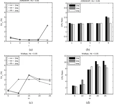
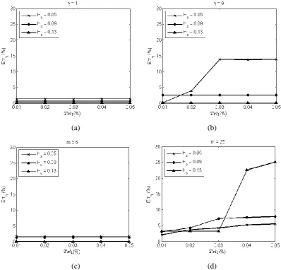
Next, we keep the significant wave height unchanged, i.e., , and test on different rogue wave heights, i.e., , and . The basic set-ups are the same with that for Fig. 3 and Fig. 4. Similar to these in the previous section, the errors of the free surface together with the CPU ratios are presented in Fig. 11 for the cases with different spectrum and
different parameters.
1 3 5 7 9
0 1 2 3 4 5 6 7 8 E rr ( % )
JONSWAP, Hs = 0.05
2Hs 3Hs 4Hs
1 3 5 7 9
0 0.5 1 1.5 2 2.5 3 3.5 4 C P U R a ti o
JONSWAP, Hs = 0.05
2Hs 3Hs 4Hs
(a) (b)
5 10 15 20 25
0 1 2 3 4 5 6 7 8 m E rr ( % )
Wallops, Hs = 0.05
2Hs 3Hs 4Hs
5 10 15 20 25
0 2 4 6 8 10 12 m C P U R a ti o
Wallops, Hs = 0.05
2Hs 3Hs 4Hs
(c) (d)
Fig. 11. and CPU ratio (CPU time of ESBI/CPU time of hybrid model) for the cases with different rogue wave heights
It shows that the errors in the cases for both the JONSWAP and Wallops spectra with
different width parameters are less than 5%, which confirms that the values for the and controlling the switch between the models are appropriate for the cases with different embedded rogue waves. It can be seen from Fig. 11(b) that the CPU time ratio is approximately 1.9 in all cases with the JONSWAP spectrum, except for the cases with
and . That is because the ENLSE-5F is involved only in these cases. When the ENLSE-5F is not involved, the calculation is switched only between the QSBI and ESBI
models. As indicated above, the QSBI use about a half of CPU time used by ESBI, which implies that the QSBI are implemented in most of time steps for the cases except for these
[image:27.595.96.486.202.554.2]27
On the other hand, for the simulations based on the Wallops spectrum, the story is
different in particular when . In these cases, the CPU time ratio is more than 8 or even 10, Fig. 11 (d), implying that the new hybrid method is very much more efficient than the ESBI only. When , the ratio is not so high, though it is still larger than 2.
In order to illustrate how the models switch during the simulation, Fig. 12 is presented in
a similar way to that for Fig. 6. It shows that in some case, the process starts with ENLSE-5F, then goes to QSBI and ESBI, ending with QSBI, e.g, Fig. 12 (a). In some other cases, the
process starts with ENLSE-5F, then goes to QSBI and ESBI, ending with ENLSE-5F, e.g, Fig. 12(d). The various scenarios illustrated in Fig. 12 demonstrate that the automatic switch
between the three models works well.
Furthermore, the profiles with the rogue wave height of at focusing time and location are shown in Fig. 13. It is found that the results obtained by using the hybrid model are almost identical with that obtained by using the ESBI only. However, the hybrid model
significantly save the CPU time with different degrees as indicated above.
(a):
28
(c):
[image:29.595.106.478.78.427.2](d):
Fig. 12. Maximum wave elevations with indicators for which model is used for the cases with different rogue wave heights
(a) (b)
Fig. 13. The profiles of the rogue wave with height of for the cases with different rogue wave heights
4.2 Different numbers of rogue waves in time domain
[image:29.595.99.482.494.664.2]29
[9] at different times. Therefore, cases with different numbers of rogue wave events in a tie domain are investigated in this section. In addition to one rogue wave event , the cases with two rogue wave events at and three rogue wave events
are studied by using the same set-ups with that for Fig. 3 and Fig. 4.
The rogue wave height is fixed to as there will not be energy left to generate the random background if three successive rogue waves higher than are generated by using the method explained in [78]. Similarly, the errors and CPU time ratios are presented in Fig. 14.
1 3 5 7 9
0 1 2 3 4 5 6 7 8 E rr ( % )
JONSWAP, Hs = 0.05
Tf/T0 = 100
Tf/T0 = 100 & 500
T
f/T0 = 100 & 500 & 900
1 3 5 7 9
0 0.5 1 1.5 2 2.5 3 3.5 4 C P U R a ti o
JONSWAP, Hs = 0.05
Tf/T0 = 100
Tf/T0 = 100 & 500
Tf/T0 = 100 & 500 & 900
(a) (b)
5 10 15 20 25
0 1 2 3 4 5 6 7 8 m E rr ( % )
Wallops, Hs = 0.05
Tf/T0 = 100
Tf/T0 = 100 & 500
T
f/T0 = 100 & 500 & 900
5 10 15 20 25
0 2 4 6 8 10 12 14 m C P U R a ti o
Wallops, Hs = 0.05
T
f/T0 = 100
Tf/T0 = 100 & 500
Tf/T0 = 100 & 500 & 900
[image:30.595.97.485.204.576.2](c) (d)
Fig. 14. and CPU ratio (CPU time of ESBI/CPU time of hybrid model) for the cases of different amount of rogue waves on temporal scale
As shown in Fig. 14 (a) and (c), the errors for all the cases considered in this section are
less than 5%, which again confirms effectiveness of the values of and for controlling the switching in the cases with different amount of rogue waves on temporal scale.
It is shown in Fig. 14(b) that for the simulations based on the JONSWAP spectrum, the
maximum CPU time ratio appears to be 2.5 for the case with , and the
ratio is about 2 in most other cases, which is largely similar to what has been observed in Fig.
30
and with are simulated mostly by the
ESBI, so that the CPU time ratio is approximately 1.2, but a little higher than 1 due to the involvement of the QSBI and ENLSE-5F.
For the simulations based on the Wallops spectrum, the CPU time ratios are all larger
than 4 except for the cases with , which are however approximately 2. Roughly
speaking, the CPU time ratio increases when the spectrum becomes narrower ( increases). Among all the cases, the most efficient case is the one that rogue wave only occurs once at
with , which leads to the CPU ratio of 9.2.
In addition, in order to examine how the hybrid model switching between each model for
the numerical examples in this section, similar graphs with Fig. 6 are presented in Fig. 15. It shows that for the cases based on the JONSWAP spectrum, the hybrid model can effectively
switch from QSBI to ESBI, and then back to QSBI during each occurrence of rogue wave, e.g., Fig. 15(a)(b). For these based on the Wallops spectrum, the hybrid model starts with ENLSE-5F, then to QSBI and/or ESBI, and switches back to ENLSE-5F before the end of the
simulations, e.g., Fig. 15(c)(d). It reveals again that the numerical technique for controlling the automatic switch between the three models is also effective for the more complicated
cases.
Furthermore, in order to show that the hybrid model successfully captured the movement
of the free surface when rogue waves occur, the free surface elevation at focusing time and location for the case , are shown in Fig. 16. It is seen that no visible
difference can be observed between the results obtained by using the hybrid model and the ESBI, which indicates that the hybrid model is very accurate.
31
(b):
(c):
(d):
[image:32.595.105.478.79.606.2]32
(a): (b):
(c): (d):
[image:33.595.95.487.73.609.2](e): (f):
Fig. 16. The profiles of the rogue waves for the cases of different numbers of rogue waves in time domain
4.3 Different numbers of rogue waves in spatial domain
Moreover, there are possibilities that several rogue waves can occur simultaneously but
at different locations [9]. Thus in this section, different numbers of rogue waves are generated at , but at different locations. In addition to the case in which a single rogue
wave occurs at , two more cases of the twins occur at and the
33
is fixed to as there will not be energy left to generate the random background if three
rogue wave higher than are generated at the same time by using the method explained in [78]. The basic set-ups are the same with that for Fig. 3 and Fig. 4. Again, the errors and the CPU time ratios are shown in Fig. 17.
1 3 5 7 9
0 1 2 3 4 5 6 7 8 E rr ( % )
JONSWAP, Hs = 0.05
X
f/L0 = 64
X
f/L0 = 32 & 64
X
f/L0 = 32 & 64 & 96
1 3 5 7 9
0 0.5 1 1.5 2 2.5 3 3.5 4 C P U R a ti o
JONSWAP, Hs = 0.05
Xf/L0 = 64
Xf/L0 = 32 & 64
X
f/L0 = 32 & 64 & 96
(a) (b)
5 10 15 20 25
0 1 2 3 4 5 6 7 8 m E rr ( % )
Wallops, Hs = 0.05
X
f/L0 = 64
Xf/L0 = 32 & 64
X
f/L0 = 32 & 64 & 96
5 10 15 20 25
0 2 4 6 8 10 12 14 m C P U R a ti o
Wallops, Hs = 0.05
X
f/L0 = 64
X
f/L0 = 32 & 64
X
f/L0 = 32 & 64 & 96
[image:34.595.95.489.161.542.2](c) (d)
Fig. 17. and CPU ratio (CPU time of ESBI/CPU time of hybrid model) for the cases of different amount of rogue waves on spatial scale
It is seen again that errors of all simulations considered in this section are less than 5%,
which confirms that the values for the and controlling the switch between the models are appropriate for the cases with different embedded rogue waves on spatial scale.
According to Fig. 17(b), for the simulations based on the JONSWAP spectrum, the CPU time ratios reach the highest, i.e., nearly 2.4~2.5, only for the cases and
with , due to the involvement of ENLSE-5F for a limited time
steps and QSBI for the most time steps. While for the cases and
with , the majority of the duration is simulated by the ESBI, so
34
alone, which leads to the CPU time ratios approximated equal to 1.3~1.4. In other cases, the majority of the duration is taken over by the QSBI, thus the CPU time ratios are about 1.8,
which indicates that the hybrid model still saves almost half the CPU time than the ESBI. Meanwhile, the situations are totally again different for the simulations based on the Wallops spectrum, as shown in Fig. 17(d), like what has been seen in Fig. 11. The hybrid
model is at least 8 time faster than the ESBI alone when . In spite of the cases for
and with , in which the CPU time ratios are
between 1~1.5, the rest of the cases when have the CPU time ratios of 2.5~4.5. The similar graphs to Fig. 6 are also presented in Fig. 18 for these cases, in order to illustrate the effectiveness of the numerical techniques for controlling the switch between
each model. It shows that the hybrid model starts with the QSBI and switch to ESBI, then back to QSBI before the end of the simulation in Fig. 18(a). Otherwise, the hybrid model
begins with ENLSE-5F, switching to QSBI and/or ESBI when rogue waves occur, then ends with ENLSE-5F or QSBI, e.g., Fig. 18(b)-(d). The various situations shown in Fig. 18 indicate that the hybrid model can start with different models and effectively switch between
each other according to the nonlinearities to achieve the highest computational efficiency. Additionally, the free surface profiles at each focusing location for the case
are shown in Fig. 19. Although the fully focusing is not achieved at in Fig. 19(b), rogue waves are observed at the rest locations. Most importantly,
the results obtained by using the hybrid model is consistent with these obtained by using the ESBI, which implies that the hybrid model has successfully captured the movement of the
free surface in the complex case.
35
(b):
(c):
(d):
[image:36.595.105.478.79.603.2]36
(a)
[image:37.595.122.471.80.623.2](b)
Fig. 19. The profiles of the rogue waves for the cases of different numbers of rogue waves in spatial domain
4.4 3D random waves simulation
As indicated above, Ducrozet et al. [29] simulated a 3D random sea covering
peak wave lengths and lasting for 250 peak wave periods by using 10 CPU days on a 3 GHz-Xeon single processor PC based on the fifth order High-order Spectral method. In order
37
wave simulation in [29] is repeated here, i.e., the computational domain and the duration of wave propagation in our simulation are all the same as in [29]. The free surface elevation is
outputted every peak period and it is shown in Fig. 20 for that at , and the statistics of the free surface at in comparison with [79] is shown in Fig. 21, which indicates that the results obtained by using the hybrid model is consistent with that in
[79]. It is noted that the statistics in [29] for the same case is different from these in [79]. By personal communication with the authors, we are informed that the data in [79] is correct for
the case. The simulation of this case is performed by using a single core on a workstation equipped with Intel(R) Xeon(R) CPU [email protected]. It is found that only the QSBI and
ESBI are involved in the simulation. The total CPU time costed by the hybrid method is 11.9 hours, which is only about 1/20 of the CPU time reported by [29]. In addition, the clock speed
of the processor used here is slower than that used by Docrozet et al. [29], which means that the CPU time of the hybrid method can be further reduced if using higher performance
[image:38.595.98.502.352.737.2]computers. It is noted that it is impossible to directly compare our wave elevation with [29] because the phase of each wave component is assigned randomly in both simulations.
Fig. 20. Free surface elevation at
[image:38.595.198.407.553.729.2]38
distribution; ‘---’ Results in [79]; ‘-■’ Results by using hybrid model
Furthermore, two cases of the 3D random sea simulation in [80] (cases (b) and (d) shown
in Figure 8 of that paper) are repeated by using the present hybrid model. Following the study in [80], the JONSWAP spectrum and a (with N=50 and 200, respectively) type
directional distribution function are used to generate the spreading seas. As an example, the free surface for at the end of the simulation (after about 60 peak periods) is shown in Fig. 22. The kurtosis estimated by the hybrid method, all larger than 3, is presented in Fig.
23, altogether with the results based on the broader-bandwidth Dysthe equation, HOS method and experimental data in [80]. As well known, the kurtosis represents the contribution of big
waves in the statistical distribution, and the contribution of the big waves is significant if it is larger than 3 [9]. It shows in Fig. 23 that the results obtained by using the hybrid model in this
paper agrees very well with that obtained based on the HOS method and experimental data in [80]. While the results obtained by using the broader-bandwidth Dysthe equation [80] are
significantly smaller. It indicates that the nonlinearities cannot be fully resolved in the simulations based only on the broader-bandwidth Dysthe equation, and in such cases, the
[image:39.595.160.456.385.530.2]fully nonlinear or the hybrid model suggested in this study should be employed.
Fig. 22. Free surface elevation at for
[image:39.595.99.481.569.723.2]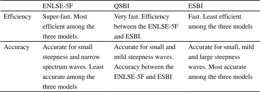
![Fig. 5. Free surface at different instant. ‘—’: Hybrid method; ‘x’ Method in [64]](https://thumb-us.123doks.com/thumbv2/123dok_us/1464683.99118/23.595.122.468.437.722/fig-free-surface-different-instant-hybrid-method-method.webp)