Numerical modelling of twin-screw pumps based on computational fluid dynamics

City, University of London Institutional Repository

Citation

:

10.1177/0954406216670684

This is the accepted version of the paper.

This version of the publication may differ from the final published

version.

Permanent repository link:

Link to published version

:

Copyright and reuse:

City Research Online aims to make research

outputs of City, University of London available to a wider audience.

Copyright and Moral Rights remain with the author(s) and/or copyright

holders. URLs from City Research Online may be freely distributed and

linked to.

City Research Online: http://openaccess.city.ac.uk/ [email protected]

Mechanical Engineering Science, doi: 10.1177/0954406216670684

Numerical Modelling of Twin-screw Pumps Based on Computational

Fluid Dynamics

Di Yan1, 2_{, Ahmed Kovacevic}2_{, Qian Tang}1*_{, Sham Rane}2_{, Wenhua Zhang}3

1 _{State Key Laboratory of Mechanical Transmission, Chongqing University, 400044, China;}

2_{Centre for Compressor Technology, City University London, EC1V0HB, UK;}

3_{Chongqing Yuejin Machinery Co.,Ltd, Yongchuan District, Chongqing, 402169, China}

Abstract

Increasing demands for high-performance screw pumps in oil and gas as well as other applications require deep understanding of the fluid flow field inside the machine. Important effects on the performance such as dynamic losses, influence of the leakage gaps, presence and extent of cavitation are difficult to observe by experiments. However, it is possible to study such effects using well validated CFD (computational fluid dynamics) models. The novel structured numerical mesh consisting of a single computational domain for moving screw pump rotors was developed to allow 3-D CFD simulation of such machine possible. Based on Finite Volume Method (FVM), the instantaneous mass flow rates, rotor torque, local pressure field, velocity field and other performance indicators including the indicated power were predicted. A calculation model for the bearing friction losses was introduced to account for mechanical losses. The geometry of the inlet and outlet passages and piping system are taken into consideration to evaluate their influences on the pressure distribution and shaft power. The paper also shows the influence of rotor clearances on the pump performance.

The CFD model was validated by comparing the numerical results with the measured performance obtained in the experimental test rig through the comprehensive experiment performed for a set of discharge pressures and rotational speeds. Validation includes comparison of mass flow rates, shaft power and efficiency under variety of speeds and discharge pressure. It has been found that the predicted results match well with the measurements. The results also showed that that the radial clearances have larger influence on the mass flow rate than the interlobe clearance. The correct design of the flow passages within the screw pump plays significant role in minimizing required power consumption.

The analysis presented in this paper contributes to better understanding of the working process inside the screw pump and offers a good reference to improve design and optimise such machines in terms of clearance selection, shape of the ports, piping system etc. In future this model will be used for analysis of cavitating flows and determining performance of other multiphase screw pumps.

Keywords：Screw Pump; CFD; Numerical modelling; Clearance; Bearing Losses

Mechanical Engineering Science, doi: 10.1177/0954406216670684

1.

Introduction

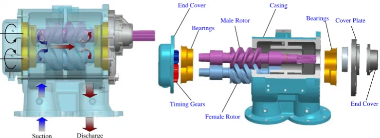
Twin screw pumps are positive displacement machines widely used in petrochemical, shipping, energy and food industries due to their reliability and excellent performance in single phase or multiphase operation. Typical arrangement of a twin screw liquid pump is given in Figure 1, showing rotors synchronised by timing gears and enclosed in the casing. Increasing demands for high-performance screw pumps require improvements in pump designs. Recent developments in manufacturing technologies allow accurate production of novel designs. But for improvements in the design of screw pumps, full understanding of process within the pump is required. To date, most of the models for their performance analysis are based on thermodynamic chamber modelling.

Timing Gears

Female Rotor Male Rotor Bearings

Bearings _{Cover Plate}

End Cover Casing

End Cover

Figure 1 Structure and components of twin-screw pump

Research work on modelling and experimental investigation of working processes in twin screw pumps was reported in many previous studies. The number of literature resources is large and therefore just the most relevant will be listed below. Li [1] introduced the structure, tooth profiles generation and performance calculation of different kinds of screw pumps. Feng C. et.al [2] built models for the back flow and pressure generation within the multiphase twin-screw pump and also simulated the thermodynamic performance and the transport behaviour of the pump with different gas volume fractions. Tang and Zhang [3] modelled the flow field dynamics based on CFD by static mesh and proposed a leakage model for twin-screw pump, they also optimized the tooth profiles. Jing Wei [4] discussed the tooth profile design of twin-screw kneader and simulated the flow field based on CFD by static grid. D. Mewes [5] proposed a performance calculation model for a multiphase pump according to the mass and energy conservation in the pump chamber and validated it by experiments. Abhay Patil [6] and Evan Chan [7] studied the steady state and transient properties under different working conditions. They discussed about the influence of the viscosity of the sealing liquid and gas void fraction on the performance of a two-phase screw pump. K. Rabiger [8] proposed a model for screw pump and carried out the numerical and experimental analysis of the performance of the pump under very high gas volume fractions (90%-99%), he also conducted an experiment to visualize the leakage flow in the radial clearance [9].

Mechanical Engineering Science, doi: 10.1177/0954406216670684

mathematical models which neglect kinetic energy and simplify the analysis of the main and leakage flows [10],[11]. Few others refer to a steady state computational fluid dynamics (CFD) which assumes static mesh of the moving flow domains. By using static mesh, approximate pressure gradients and the leakage velocity field can be obtained; however such results do not take into account the velocity field of the main flow and neglect the transient nature of the working process in a screw pump. Due to the limitation of CFD simulation using static mesh, some important parameters cannot be obtained, such as the mass flow rate, rotor torque and pressure fluctuation. More so, in the case of a multiphase pump the pressure field will differ significantly from the result obtained on a static mesh and therefore power calculation will be inaccurate. In addition the pressure flow losses could not be calculated. Therefore phenomena such as power losses, effect of change in clearances and any dynamic behaviour including cavitation and multiphase flows could not be analysed using such static mesh.

The working domain of a screw pump is formed between moving rotors and stationary casing. It changes the shape and size with the rotation of the rotors. In order to obtain the pressure, temperature and velocity fields by use of CFD, the numerical mesh needs to deform in time accurately following the shape of the working domain. The numerical grid generators commonly implemented in the commercial CFD software are unable to fulfil these requirements and a specialised grid generator is required.

Breakthrough in using CFD for analysis of positive displacement screw machines was made by Kovacevic [12] who generated structured moving mesh for screw compressors based on a rack generation method proposed by Stosic [13]. This pioneering work in grid generation for screw machines allowed for the CFD simulation and performance prediction for screw compressors [14]. This method provided a powerful basis for research of screw pumps.

Screw pumps and screw compressors are similar in configuration but aside of the rotor profile geometry there are other differences which affect simulation. Firstly, working fluid for pumps is either liquid or multiphase fluid consisting mainly of liquid and some gas. Secondly, the pump working processes usually does not include internal compression of the gas and therefore temperatures in screw pump are not changing that rapidly. Finally, inlet and outlet ports are different. The inlet and outlet ports in screw pump are usually designed as an open type for easier suction and discharge.

In this paper, a conformal structured moving mesh is generated for the rotor fluid domain. The polyhedral mesh is used for ports and pipes. Handling of the structured moving mesh in the CCM solver is managed by use of the UDF and interface program made specially for handling conformal rotor mesh which will be described later in the paper.

Mechanical Engineering Science, doi: 10.1177/0954406216670684

2.

Mathematical Model

Positive displacement screw pumps operate on the basis of changing the size and position of a working domain which consequently causes change in the pressure of the domain which causes transports of the fluid. To calculate performance of such a pump, quantities such as mass, momentum, energy etc. need to be modelled. Conservation of these quantities can be represented by a general transport equation for a control volume (1), [15]

𝜕

𝜕𝑡∫ 𝜌𝜙𝑑𝛺_𝛺

𝑡𝑟𝑎𝑛𝑠𝑖𝑒𝑛𝑡

+ ∫ 𝜌𝜙𝒗 ∙ 𝒏𝑑𝑆 =_𝑆

𝑐𝑜𝑛𝑣𝑒𝑐𝑡𝑖𝑜𝑛

∫ 𝛤 𝑔𝑟𝑎𝑑 𝜙 ∙ 𝒏𝑑𝑆

𝑆

𝑑𝑖𝑓𝑓𝑢𝑠𝑖𝑜𝑛

+ ∫ 𝑞𝜙𝑠𝑑𝑆

𝑆

𝑠𝑜𝑢𝑟𝑐𝑒

+ ∫ 𝑞𝜙𝑣𝑑𝛺

𝛺

𝑠𝑜𝑢𝑟𝑐𝑒

(1)

In order to account for the deformation of the working domain, the conservation equation (1) needs to account for the velocity of the domain boundary. This could be done by replacing the velocity in the convective term with the relative velocity (𝒗 − 𝒗𝒃), where 𝒗𝒃 is the velocity

vector at the cell face. In such case, the general conservation equation can be written as, 𝑑

𝑑𝑡∫ 𝜌𝜙𝑑𝛺_𝛺

𝑡𝑟𝑎𝑛𝑠𝑖𝑒𝑛𝑡

+ ∫ 𝜌𝜙(𝒗 − 𝒗𝒃) ∙ 𝒏𝑑𝑆 =

𝑆

𝑐𝑜𝑛𝑣𝑒𝑐𝑡𝑖𝑜𝑛

∫ 𝛤 𝑔𝑟𝑎𝑑 𝜙 ∙ 𝒏𝑑𝑆

𝑆

𝑑𝑖𝑓𝑓𝑢𝑠𝑖𝑜𝑛

+ ∫ 𝑞𝜙𝑠𝑑𝑆

𝑆

𝑠𝑜𝑢𝑟𝑐𝑒

+ ∫ 𝑞𝜙𝑣𝑑𝛺

𝛺

𝑠𝑜𝑢𝑟𝑐𝑒

(2)

The grid velocity 𝒗𝒃and the grid motion are independent of the fluid motion. However, when

the grid velocities are calculated explicitly and used to calculate the convective fluxes, the conservation of mass and other conserved quantities may not necessarily be preserved. To ensure full conservations of these equations, the space conservation law needs to be satisfied as given by (3).

𝑑

𝑑𝑡∫ 𝑑𝛺_𝛺 − ∫ 𝒗_𝑆 𝒃∙ 𝒏𝑑𝑆 = 0 (3)

Space conservation can be regarded as mass conservation with zero fluid velocity. The unsteady terms in the governing equations involving integration over a control volume 𝛺, which is now changing with time, need to be treated in a way consistent with the space conservation equation with a deforming and/or moving grid.

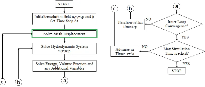
Figure 2 Flow chart of solution process with deforming domains

Mechanical Engineering Science, doi: 10.1177/0954406216670684

of partial differential equations (PDE’s) and often employ a Finite Volume Method (FVM) to be solved.

Figure 2 represents a flow chart of the solution process for a FVM with deforming domains. The highlighted step for resolving the mesh displacement is crucial for ensuring space conservation which requires the grid velocities and changes in CV volumes to be known at each new time step.

Providing that the numerical mesh used for transient calculation of a screw pump has a structured topology with the constant number of computational cells for any rotor position, then the movement of vertices which define the mesh can be used for calculation of wall velocity 𝒗𝒃 ensuring that the space conservation and the entire solution are fully conservative [16].

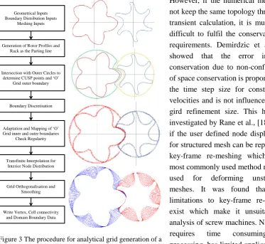
However, if the numerical mesh does not keep the same topology throughout transient calculation, it is much more difficult to fulfil the conservativeness requirements. Demirdzic et al., [17] showed that the error in mass conservation due to non-conformance of space conservation is proportional to the time step size for constant grid velocities and is not influenced by the gird refinement size. This has been investigated by Rane et al., [18] to test if the user defined node displacement for structured mesh can be replaced by key-frame re-meshing which is the most commonly used method normally used for deforming unstructured meshes. It was found that many limitations to key-frame re-meshing exist which make it unsuitable for analysis of screw machines. Namely, it requires time consuming pre-processing, has limited applicability to complex meshes and leads to inaccuracies in conservation of calculated variables. It was therefore concluded that customized tools for generation of CFD grids are required for screw pumps as earlier elaborated in [14]. Grid generation is a process of discretising a working domain of the screw pump in control volumes for which a solution is to found. It may be numerical, analytical or variational, as outlined in [14]. The results obtained in this research work used grids generated by analytical grid generation. Applying the principles of analytical grid generation through transfinite interpolation with adaptive meshing, the authors have derived a general, fast and reliable algorithm for automatic numerical mapping of arbitrary twin screw machine geometry [19],[25]. On that basis, the authors have developed a program called SCORG (Screw COmpressor Rotor Geometry Grid generator), which enables automatic rotor profiling, grid generation and direct

Geometrical Inputs Boundary Distribution Inputs

Meshing Inputs

Generation of Rotor Profiles and Rack as the Parting line

Intersection with Outer Circles to determine CUSP points and ‘O’

Grid outer boundary

Boundary Discretisation

Adaptation and Mapping of ‘O’ Grid inner and outer boundaries

Check Regularity

Transfinite Interpolation for Interior Node Distribution

Grid Orthogonalisation and Smoothing

Write Vertex, Cell connectivity and Domain Boundary Data

Figure 3 The procedure for analytical grid generation of a

Mechanical Engineering Science, doi: 10.1177/0954406216670684

connection with a number of CFD solvers. More detail could be found in [14].

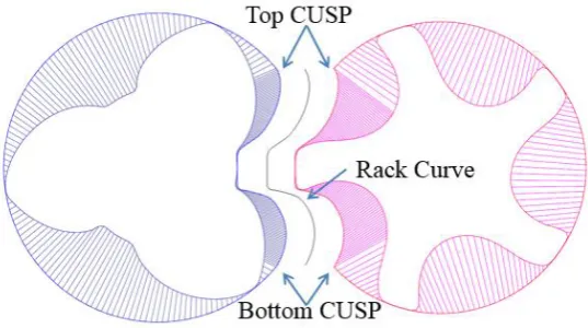
The procedure of analytical grid generation of screw pump machine working domain is shown in Figure 3. In order to achieve a conformal single domain mesh of the moving elements which is required for a number of solvers, the rotor flow domain is initially divided into two subdomains belonging to two rotors using the rack plane which can be generated analytically or numerically using Willis meshing conditions. Following that the main steps of mesh generation in each cross section are [20]:

 Outer boundary in each block is defined as a combination of the rack segment and the casing circle segment. The rack segment stretches between the bottom CUSP point to the top CUSP point and is closed by the casing as shown in Figure 5.

 Rack segment is discretized using equidistant distribution. It is possible to use same distribution for both subdomains in order to maintain conformal interface if required.

 Casing segment in each subdomain is discretized using equidistant distribution which is usually different than for the rack segment. The distribution obtained on the outer boundaries of the two blocks is the reference for the rotor profile distribution.

 Nodes are distributed on the rotor profile with corresponding distribution available on the outer boundary. It is very likely that at first the initial cells will overlap for helical rotors, especially on the face of the gate rotor profile.

 Distribution on rotor profiles is regularized using background blocking.

 Interior nodes are distributed using transfinite interpolation.

 Orthogonalisation and smoothing iterations are performed to improve cell quality.

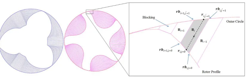
Blocking is a uniform distribution of nodes on the rotor profile and on the outer circle as shown in Figure 4.

The advantage of such blocks is that:

 Blocks do not have to be as refined as the final grid.

 Blocks can be used as reference for refinement in any required regions.

 Blocks have to be calculated only once and simply rotate for various rotor positions.

Figure 4 Background blocking for the main and gate rotors

Suppose that the points distributed on the boundaries are represented in index notation with respect to the physical coordinate system as ri,j (x,y). Points on the rotor profile are ri,j=0 (x,y),

points on the outer boundary consisting of casing and rack curve are ri,j=1 (x,y) and the point

distribution on outer full circle is ri,j’=1 (x,y). Each of the background blocks is identified by its index Bi. The points on the inner boundary of the blocks which are the rotor profile nodes are

Mechanical Engineering Science, doi: 10.1177/0954406216670684

Starting from the bottom CUSP, nodes are distributed on the outer circle covering the rack part with required number of points irack. Nodes are then distributed on the outer circle covering the

casing part with required number of points icasing. At this stage the data are available for rbi,j=0

(x,y), rbi,j’=1 (x,y) and ri,j’=1 (x,y) and it is required to calculate ri,j=0 (x,y). This node distribution

is based on equidistant spacing as given in equation (4).

𝒓_𝑖,𝑗′₌₁(𝑥, 𝑦) = 𝒓_{𝑖−1,𝑗}′₌₁(𝑥, 𝑦) + 𝑆_𝑖 𝑖 (4)

𝑆_𝑖 =𝑆I

I

𝑆_𝐼 = 𝒓_𝐼,𝑗′₌₁(𝑥, 𝑦) − 𝒓_𝑖=0,𝑗′₌₁(𝑥, 𝑦)

A scanning function is introduced that has the information of the background blocking. Starting from the bottom CUSP, the scanning function traces each node ri,j’=1 (x,y) and identifies

the block Bi to which it belongs. There can be situation when a single block has multiple nodes

present in it or there can be blocks with no nodes present. This is because the distribution on the rack curve can be refined in comparison to the blocking. Similarly the distribution on the casing can be coarse in comparison with the blocking. Once the nodes associated with each block are traced by the scanning function, an arc-length based projection is used to determine the nodes ri,j=0 (x,y) to be placed on the rotor profile. At the same time constraint is imposed on

the node placement that they have to be bound in the same block 𝐁𝑖 Bi as that of the outer circle

nodes ri,j’=1 (x,y).

Figure 4 shows the projection of ri,j’=1 (x,y) on the inner boundary of the block in order to

get ri,j=0 (x,y). This projection is based on arc length factor given by equation (5).

𝒓_𝑖,𝑗=0(𝑥, 𝑦) = 𝒓𝒃𝑖,𝑗=0(𝑥, 𝑦) + (𝒓𝒃𝑖+1,𝑗=0(𝑥, 𝑦) − 𝒓𝒃𝑖,𝑗=0(𝑥, 𝑦))

𝑆𝑖

𝑆𝐼

(5)

𝑆_𝑖 = 𝒓_𝑖,𝑗′₌₁(𝑥, 𝑦) − 𝒓𝒃_𝑖,𝑗′₌₁(𝑥, 𝑦)

𝑆𝐼= 𝒓𝒃𝑖+1,𝑗′₌₁(𝑥, 𝑦) − 𝒓𝒃_𝑖,𝑗′₌₁(𝑥, 𝑦)

The calculated positions ri,j=0 (x,y) of nodes ensure that they are guided by a regular rotor profile. Regularised distribution is superimposed onto the rack curve by finding the intersection points of the distribution lines and the rack curve. These intersection points are the new distributions ri,j=1 (x,y) on the rack curve as shown in Figure 5.

Figure 5 Refinement in the rack segment and superimposition of rack curve

Mechanical Engineering Science, doi: 10.1177/0954406216670684

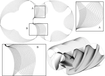
non-identical. Depending on this the results is a conformal or non-conformal map between the two rotor blocks respectively. With the blocking approach the 3D grid is fully hexahedral and both the main and the gate rotor surfaces are smoothly captured as shown in Figure 6. At the transition point from interlobe region to the casing region small non-aligned node movements are possible. However, these are positioned on the surface of the rotors and do not result in any irregular cells. The surface mesh on the casing is of the highest quality with regular quadrilateral cells. The surface mesh on the interlobe interface mostly follows axial grid lines with only small transverse movements in the vicinity of the top and bottom CUSP’s which are cyclically repeating. These movements are on the surface of the interface and do not result in any irregular cells. The current implementation allows for a fully conformal interface with the equal index of the top and bottom CUSP points which ensures straight line in the axial direction [20].

Figure 6 Grid generated with background blocking in screw compressor rotor

3.

Setup for calculation of the liquid screw pump

The screw pump used for this study shown in Figure 1 is a twin-screw pump with a 2/3 lobe arrangement and A-type profile rotors. The operating speed on male rotor changes from 630 to 2100 rpm while keeping the discharge pressure as 0.85 MPa. By controlling the valve, the discharge pressure varies from 0.35 to 0.85 MPa while keeping rotation speed of male rotor as 2100 rpm. The male rotor diameter and the female rotor are 140.00 mm while the centre distance between two rotors is 105.00 mm. The length of the rotors is 200.00mm and the male rotor has a wrap angle of 590.0°.

3.1 Grid generation

Mechanical Engineering Science, doi: 10.1177/0954406216670684

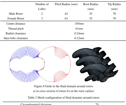
shown as Figure 8. Configuration of the mesh around rotors is given by Table 2.

Figure 7 A-type tooth profile used in this paper

Table 1 Geometry parameters of screw rotors used in study

Number of

Lobes

Pitch Radius (mm) Root Radius

(mm)

Tip Radius

(mm)

Male Rotor 2 42 35 70

Female Rotor 3 63 35 70

Centre distance 105mm

Thread pitch 61mm

Radial clearance 0.24mm

Inter-lobe clearance 0.12mm

Figure 8 Grids in the fluid domain around rotors

a) in cross section of rotors b) on the rotor surface

Table 2 Mesh configuration of fluid domains around rotors

Circumferential divisions 75

Radial divisions 7

Axial divisions 75

Interface divisions 78

Number of profile points 1000

Mechanical Engineering Science, doi: 10.1177/0954406216670684

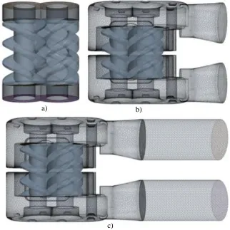
influence of geometry of the ports on the performance of screw pump, three sets of suction and discharge have been used respectively in the calculation in order to study the influence of the inlet and outlet flow domains on the accuracy of performance predictions.

1. The first set of meshes that use only two the immediate axial ports are shown in Figure 9a. In this case the extended ports and pipe system are not considered.

2. The second case includes the extract full ports which include two parts: full inlet port and out port (see Figure 9b).

3. Based on the full ports in Figure 9, two pieces of pipes are added to connect with each port (Figure 9c). Because in reality, there is usually a distance between the pumps and testing meters. This geometry presents the calculation with ports and pipes.

a) _b)

c)

Figure 9 Variations of the port geometry used in calculation

a) (top left) basic ports; b) (top right) complete port domains excluding the pipes;

c) (bottom) complete port domains including the pipes

A numerical mesh used in this study compromises 1079757 cells of which 775180 cells represent the fluid domain between the rotors, 293648 cells represent the two ports while 10929 cells represent the pipes.

3.2 Numerical Methods

Mechanical Engineering Science, doi: 10.1177/0954406216670684

for the relaxation scheme which provides better convergence by iteratively correcting (relaxing) the linear equation during multigrid cycling.

The main rotor rotates 2.4° per step. The mesh is updated before commencing solution for each time step. The time-step is defined as follows:

t = 𝐷𝑃𝑇𝑆

6 ∙ 𝑅𝑃𝑀 (6)

whereby, 𝐷𝑃𝑇𝑆 is the degree per time step, 𝑅𝑃𝑀 is the rotation speed of male rotor. When the 𝐷𝑃𝑇𝑆 is not small enough, it will make the simulation run with a relatively large time-step which may cause the divergence of calculation. Here, 𝑡 is inversely proportional to 𝑅𝑃𝑀, which means that the mesh has to be changed for different 𝑅𝑃𝑀 in order to keep the ratio of time and spatial step constant. It’s not always essential to keep the ratio constant but it is limited by Courant stability condition [14].

The k- turbulence model is adopted in the calculation. Different turbulence models have been compared during this simulation and will be described in another publication. Stagnation inlet and pressure outlet are used respectively for the inlet and outlet boundaries. The pressure of the inlet port is 0 Pa. The discharge pressure ranges from 0.35 to 0.85MPa while the rotation speed of the male rotor ranges from 630 to 2100 rpm. The initial pressure and initial velocity are 0 Pa and 0 m/s respectively. The turbulence intensity is 1% and the turbulence viscosity ratio is 10.

4.

Simulation Results

The calculations were carried out in a computer powered by 4 Intel 3.00 GHz processors and 8 GB memory. Screw pump rotation was simulated by means of 75 time steps for one interlobe rotation, which was equivalent to 150 time steps for one full rotation of the male rotor. The time step length was synchronised with a rotation speed of 630 to 2100 rpm. An error reduction of 4 orders of magnitude was required, and achieved in 50 inner iterations at each time step, each of which took approximately 3 minutes of computer time when using 4-core parallel computing on local host. However, in the beginning, it took nearly 70 minutes to generate map of the files. The overall performance parameters such as chamber pressure, velocity distribution, rotor torque, mass flow rate and shaft power were then calculated.

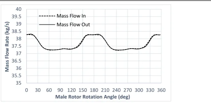
4.1 Mass Flow Rate

Mechanical Engineering Science, doi: 10.1177/0954406216670684

Figure 10 Mass flow rate vs Angle diagram

4.2 Torque

Figure 11 shows the torque of the screw pump male and female rotors. The fluctuation of torque is small. The torque on female rotor is relatively small making just about 1/14 of the torque on male rotor.

Figure 11 Torque-Angle diagram

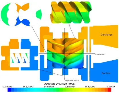
4.3 Pressure

Figure 12 shows the pressure distribution in the working domain of the screw pump. The pressure scale is chosen as 0.0 to 1.1 MPa which would give better gradients and colours. The large pressure gradient between the rotors shows the sealing line which separates the high-pressure area and low-high-pressure area. The high-pressure in the inlet port shows values below the due to the suction ability of the pump.

By monitoring the pressure in different points in the working chamber, the pressure vs angle of rotation diagram is calculated for variety of discharge pressures and speeds. Figure 13 shows the pressure history for a constant speed and discharge pressures varying from 0.35 to 0.85 MPa.

35 35.5 36 36.5 37 37.5 38 38.5 39 39.5 40

0 30 60 90 120 150 180 210 240 270 300 330 360

M

ass

Fl

o

w

R

ate

(kg

/s)

Male Rotor Rotation Angle (deg)

Mass Flow In Mass Flow Out

-30 0 30 60 90 120 150 180 210

0 30 60 90 120 150 180 210 240 270 300 330 360

To

rq

u

e o

f R

o

to

rs

(N

-m)

Male Rotor Rotation Angle (deg)

Mechanical Engineering Science, doi: 10.1177/0954406216670684

Figure 12 Pressure distribution in the working domain of the screw pump

The pressure-angle diagram shows the step change in the internal pressure through the three levels: low pressure, middle pressure and high pressure. The diagram in Figure 13 was obtained with the basic ports as shown in Figure 9a. A small variation in pressure is visible in the low pressure region just before the step between the low and middle pressure. However, this instability was reduced when full ports were applied in the calculation. It indicates that the inlet and outlet ports influence the pressure distribution within the rotors.

Figure 13 Pressure-Angle diagram for different discharge pressures

a) (left) using just basic port geometry; b) (right) using full port geometry including pipes

0 0.1 0.2 0.3 0.4 0.5 0.6 0.7 0.8 0.9 1

90 110 130 150 170 190 210 230 250 270 290

P

re

ss

u

re

(M

P

a)

Male Rotor Rotation Angle (deg) 0.85MPa 2100RPM

0.75MPa 2100RPM 0.65MPa 2100RPM 0.55MPa 2100RPM 0.45MPa 2100RPM 0.35MPa 2100RPM

0 0.1 0.2 0.3 0.4 0.5 0.6 0.7 0.8 0.9 1

90 110 130 150 170 190 210 230 250 270 290

P

re

ss

u

re

(M

P

a)

Male Rotor Rotation Angle (deg) 0.85MPa 2100RPM

Mechanical Engineering Science, doi: 10.1177/0954406216670684

4.4 Velocity

Figure 14 shows the velocity distribution in two cross sections in the working chamber. It can be seen that local high velocities are present in the radial and interlobe clearances and in the blow-hole area. The different degree of vorticity is visible in the inlet and outlet ports. The vorticity in the discharge port is comparatively higher than in the suction port due to the higher pressure in this area.

Figure 14 Velocity field in screw pump

4.5 Bearing Friction Power Losses

Screw pump rotors are normally supported by two pairs of hydrodynamic sliding bearings. Friction power losses make a significant portion of the total power dissipation which needs to be taken into account when evaluating the performance of a screw pump.

Many different empirical formulas for calculation of bearing friction losses exist [21], each of which contains experimental or empirical coefficients. The sliding bearings in this paper are fully immersed in the working medium, in this case lubricating oil. The calculation model of sliding bearing friction power introduced in this paper is based on the dynamic viscosity, eccentricity, clearance and speed of the rotor which contains no coefficients and is therefore convenient to be applied. It has been experimentally validated for this type of the bearings [22].

𝑃 = 𝐹𝑣 = 2𝜋𝜇𝑣

2_𝑟𝑙

Mechanical Engineering Science, doi: 10.1177/0954406216670684

Where, 𝜇 [P𝑎 𝑠] is the dynamic viscosity of the lubricating oil, 𝑣 [𝑚_𝑠] is the peripheral speed

of the bearing journal, 𝑙 [m] is the bearing width, 𝑐 [m] is the bearing clearance and 𝜀 [m] is the bearing eccentricity.

That friction power is assumed to be proportional to the square of the rotation speed and is not a function of the discharge pressure. Calculation results for bearing losses for variety of speeds and pressures are shown in Figure 15.

Figure 15 Bearing Friction Power – (left) vs rotational speed, (right) vs discharge pressure

Figure 16 Proportion of bearing losses in the total power

It can be seen from Figure 15 that the friction power is small at low rotation speed. Under 630rpm, it is less 0.3KW. It increases to more 5% of the total calculation power when rotation speed reaches 2100rpm and cannot be neglected, as can be seen in Figure 16.

The increase in the proportion of bearing friction losses in the total power of the screw pump linearly increases with the rotational speed. The proportion of bearing friction power decreases with the increasing discharge pressure at constant speed Figure 16. For the lowest analysed discharge pressure of 0.35 MPa and the highest analysed speed of 2100 rpm, bearing loses exceed 10% of the total power.

4.6 Study on grid independency

In order to obtain grid independent solution and to investigate the influence of the mesh size on the calculation accuracy, three different mesh sizes of the rotor fluid domain have been used to obtain the performance of the screw pump. The mesh configurations used in the calculation are shown in Table 3.

0 0.5 1 1.5 2 2.5 3

630 840 1050 1260 1470 1680 1890 2100

B ear ing Fr ic ti o n P o we r (KW )

Rotation Speed [rpm] Bearing Friction Power vs Rotation Speed

@ 0.85 MPa

1.5 2 2.5 3

0.35 0.45 0.55 0.65 0.75 0.85

B ear ing Fr ic ti o n P o we r (KW )

Discharge Pressure [MPa] Bearing Friction Power vs Pressure

@ 2100 rpm

0 1 2 3 4 5 6

630 840 1050 1260 1470 1680 1890 2100

P er ce nt ag e ( %)

Rotation Speed [rpm]

Proportion of Bearing Losses in Total Power@ 0.85MPa 0 2 4 6 8 10 12

0.35 0.45 0.55 0.65 0.75 0.85

P er ce nt ag e ( %)

Discharge pressure [MPa] Proportion of Bearing Losses in Total Power

Mechanical Engineering Science, doi: 10.1177/0954406216670684

Table 3 The mesh size for the same screw rotors

Circumferen tial divisions Radial divisions Axial divisions Interface divisions Number of cells 4-core Parallel Calculation time for 2 full rotations

Grid 1 75 7 75 78 775180 970 minutes

Grid 2 125 9 75 90 1662570 1340 minutes

Grid 3 200 12 75 100 2216760 1570 minutes

Grid 1 Case can be calculated using a computer powered by 4 Intel 3.00 GHz processors and 8 GB memory. However, 8 GB memory is not sufficient for the Grid 2 Case and Grid 3 Case. Here, a workstation with 16 Intel processors and 32 GB memory station was used for the study of grid independency.

Figure 17 (top) Mass flow rate; (bottom) Chamber pressure with different mesh sizes 150 151 152 153 154 155 156 157 158 159 160

0 30 60 90 120 150 180 210 240 270 300 330 360

M ass Fl o w R ate (m3/ h )

Male Rotor Rotation Angle (deg)

Grid 1 Grid 2 Grid 3

0 0.1 0.2 0.3 0.4 0.5 0.6 0.7 0.8 0.9 1 1.1

90 110 130 150 170 190 210 230 250 270 290

Pr e ssur e ( M Pa)

Male Rotor Rotation Angle (deg)

Mechanical Engineering Science, doi: 10.1177/0954406216670684

The results of calculations are presented in Figure 17 in the form of a discharge flow-angle diagram and a pressure-pressure diagram.

The Mass flow rate vs Angle diagram in Figure 17 shows that the mass flow rate increases with the increase in the mesh size. The difference in mass flow rate between the coarse Grid 1 and medium Grid 2 is small, 0.89%. The difference between the medium Grid 2 and Fine Grid 3 is even smaller 0.5%. The overall difference between the coarse and the fine mesh is less than 1.5%. It is expected that by doubling the mesh the difference between that grid and Grid 3 would be less than 1%. However due to the capacity of the available computing equipment, it was impossible to perform that calculation in the reasonable time. For the full grid independency it would be necessary to perform calculation on two more refined meshes of which the finest will have in access of 10 million cells which is not feasible on the computing equipment available for this research work.

The Chamber pressure-Angle diagram in Figure 17 (bottom) shows no obvious difference in power between the three calculated grids. Some oscillations in the chamber pressure are noticed with the largest number of cells (Grid 3) which could be associated with more accurate capturing of pressure oscillations. However, this will require further investigation which will be reported in future publications.

Figure 18 Shaft power obtained with different mesh sizes

Figure 18 shows the shaft power under different working conditions obtained on the three grids with progressively higher number of cells. It indicates that the power remains virtually the same for all three mesh sizes.

The calculation results of the liquid screw pump performance obtained with the three different mesh sizes show that use of an average mesh size of around 800000 cells in the rotor fluid domain can provide sufficient accuracy and reasonable computing time.

10 15 20 25 30 35 40 45 50

500000 1000000 1500000 2000000 2500000

Sh

aft Po

we

r (

kW)

Number of cells

Mechanical Engineering Science, doi: 10.1177/0954406216670684

5.

Validation of Performance calculation by experimental results

5.1 Experimental setup

Figure 19 shows the diagrammatic layout of the test rig with the main components and the photograph of the test rig used for obtaining experimental results for validation. Table 4 shows the accuracy of the measuring devices used in the experiment.

n m D

~

10 11 12

4

3 2

1 9

5 8

7

6

1 Screw Pump 2 Torque Meter and Revolution Meter 3 Motor 4 Filter 5 Cooler 6 Oil Tank 7 Filter 8 Valve 9 Vacuum Meter

10 Pressure Gauge 11 Valve 12 Flow Meter

Figure 19 The experimental setup for screw pump performance measurements

Table 4 Accuracy of instrumentation used in performance measurements

Measured value Instrument used Accuracy

Speed measurements Revolution Meter < ±0.5%

Torque Torque Meter < ±1.5%

Pressure Pressure Gauge ≤ 1.6%

Temperature Thermometer < ±1℃

Flow rate Flow Meter ≤ 0.5%

The working medium used in experiment is CD40 lubricating oil. The density is 889kg/m3 _and

the dynamic viscosity is 5.25×10-2 _{Pa∙S. The temperature of oil is 50 to 70℃. The nominal}

interlobe clearance (between two rotors) is 0.12 mm, the nominal radial clearance (between rotor and casing) is 0.24 mm.

5.2 Comparison of the results and discussion

Mechanical Engineering Science, doi: 10.1177/0954406216670684

formation of cavitation bubbles. Cavitation brings bubbles in the pump chamber, which reduces the volume of liquid during the transport of fluid. Therefore the mass flow rate will be reduced accordingly. In this calculation, multiphase model and cavitation model are not included, which will be discussed in another paper. So, when rotation speed increased to 2100rpm, the calculation results show slightly higher mass flow rate than experiment.

Figure 20 Mass flow rate: (top) variable rotational speed, (bottom) variable discharge pressure

It also can be shown that mass flow rates are basically independent of the geometry of the ports and pipes used for simulation. It can be concluded that the geometry of the inlet port and outlet port has very little influence on the mass flow rate.

Figure 21 shows the change in the shaft power under variable rotational speeds and variable discharge pressures. The calculation results match well with the experimental data. By comparison, the influence of geometry of inlet and outlet ports on shaft power has been observed. The shaft power calculated for cases which include full geometry of the ports matches closely with the experiment. It is concluded that the reality of ports has large influence on the pressure distribution in the working chamber and influences the torque accordingly. The pipes connected to the ports have a small influence on the shaft power and do not show large pressure drop within them.

0.0 20.0 40.0 60.0 80.0 100.0 120.0 140.0 160.0

420 630 840 1050 1260 1470 1680 1890 2100 2310

Fl

o

w

(m

3

/h

)

Rotor Speed (rpm) Flow vs Speed

0.85MPa Exp.

0.85MPa without ports

0.85MPa with ports

0.85MPa with ports and pipes

120.0 130.0 140.0 150.0 160.0 170.0 180.0 190.0

0.25 0.35 0.45 0.55 0.65 0.75 0.85 0.95

F

lo

w

(m

3

/h

)

Discharge Pressure (MPa) Flow vs Discharge Pressure

2100rpm Exp.

2100rpm without ports

2100rpm with ports

Mechanical Engineering Science, doi: 10.1177/0954406216670684

Figure 21 Mass flow rate: (top) variable rotational speed; (bottom) variable discharge pressure

The bearing friction losses play significant role in the prediction of power of the pump. The larger influence is noticeable for higher speeds and this follows the trend of measurements very well. The sealing friction losses are not taken into account and it is believed that these could make sufficient difference to bring power predictions even closer to the experiment.

5.3 Effect of the clearance size on leakage losses

Generally, four types of leakage gaps affect the efficiency of screw machines, namely interlobe, radial, blow-hole and end-rotor clearance gaps. Due to the open type of ports, the end-rotor clearance gaps do not exist in the screw pumps. Blow-hole area is the function of the rotor profile and for involute profiles like this one used in the screw pump, it is large. However, the influence of this leakage gap upon the performance cannot be evaluated without the change in the rotor profile. For the calculation of the pump performance, the interlobe clearance was set to 0.12 mm and the radial clearance is set to 0.24mm, which is in Figure 22 marked as 0.12 0.24. These two leakage gaps are be influenced by the manufacturing error, assembly error, position of the bearings and temperature. It is therefore difficult to estimate real operating

0.0 10.0 20.0 30.0 40.0 50.0 60.0

420 630 840 1050 1260 1470 1680 1890 2100 2310

S h af t P o w er (k W )

Rotor Speed (rpm) Shaft Power vs Speed

0.85MPa Exp.

0.85MPa without ports

0.85MPa with ports

0.85MPa with ports and pipes

0.85MPa with ports and bearing losses

0.0 10.0 20.0 30.0 40.0 50.0 60.0

0.25 0.35 0.45 0.55 0.65 0.75 0.85 0.95

S h af t P o w er (k W )

Discharge Pressure (MPa) Shaft Power vs Discharge Pressure

2100rpm Exp. 2100rpm without ports 2100rpm with ports 2100rpm with ports and pipes

Mechanical Engineering Science, doi: 10.1177/0954406216670684

clearance during the working process which was the reason to set the initial clearance to the theoretical assembly values.

The decrease of clearances can increase the mass flow rate and volumetric efficiency, on the contrary, the enlargement of clearances will bring larger leakage amount [23],[24]. In order to investigate the effects of the different clearance size on the mass flow rate, the interlobe clearance and radial clearance are varied by 0.06mm and investigates separately, The case indicated with 0.18 and 0.24 reflects the size of interlobe and radial clearance gaps respectively. The calculation results with variable clearances are shown in Figure 22.

Figure 22 Mass flow rate: (top) variable rotation speed, (bottom) variable discharge pressure

The decrease in the mass flow rate is of the order of 1.6% for 630rpm and 0.4% for 2100rpm when the interlobe clearance increased by 0.06mm. However, with the increase in radial clearance by 0.06mm, the decrease in mass flow rate is larger, 7.7% for 630rpm and 1.7% for 2100rpm.

With the increase in interlobe clearances for 0.06 mm, the mass flow rate decreased by 0.2% for 0.35 MPa and by 0.4% for 0.85MPa. However, with the increase in radial clearances by 0.06 mm, the decrease in mass flow rate is higher; the mass flow rate decreased by 0.7% for 0.35 MPa and by 1.7% for 0.85MPa.

The data comparison indicates that the leakage flow reduces with the increase in the rotational speed, while it increases with the increase in the discharge pressure. Compared with the

20.0 40.0 60.0 80.0 100.0 120.0 140.0 160.0

420 630 840 1050 1260 1470 1680 1890 2100 2310

M ass F lo w Ra te (m 3 /h )

Rotor Speed (rpm) Flow vs Speed

0.85MPa Exp.

0.85MPa 0.12 0.24

0.85MPa 0.18 0.24

0.85MPa 0.12 0.30

120.0 130.0 140.0 150.0 160.0 170.0 180.0 190.0

0.25 0.35 0.45 0.55 0.65 0.75 0.85 0.95

M ass F lo w Ra te (m 3 /h )

Discharge Pressure (MPa) Flow vs Discharge Pressure

2100rpm Exp.

2100rpm 0.12 0.24

2100rpm 0.18 0.24

Mechanical Engineering Science, doi: 10.1177/0954406216670684

interlobe clearances, the radial clearances have larger effect on the leakage losses. This study provides a good guidance for the clearance design in screw pumps.

6.

Conclusions

A full 3D CFD simulation of twin-screw pump has been carried out using structured moving numerical mesh with the conformal interface between the rotor domains based on FVM. The calculation results were validated with experimental data, to confirm the accuracy and applicability of this numerical method for performance prediction of screw pumps.

1. The progressively increasing reality of the suction and discharge were analysed in this research. It was shown that the port geometry has little effect on the mass flow rate but have significant effect on the power. More real ports used in CFD provide performance prediction which closer matches the measured data. The short pipes connected to the ports have little effect on the performance.

2. The relative leakage flow reduces with the increase in rotational speed. It increases with the increase in the discharge pressure. The radial clearances have larger effect on the mass flow rate than the interlobe clearance.

3. The difference between the measured and calculated mass flow rates decreases with the increase in speed. When the rotational speed reaches 2100rpm, the experimental mass flow rate is lower than the calculated one. The screw pump operates and virtually constant temperature so the thermal effects can be ruled out. It is believed that the reason for this trend is cavitation which appears in working chamber in the low pressure side due to the low local pressure area with the higher rotation speed. It is recommended that the effect of cavitation on the performance of the screw pump is investigates in future studies.

4. The grid independency study shows that a relatively coarse mesh can be used to obtain reasonably accurate prediction of a screw pump performance. The CFD simulation on that mesh with nearly 800000 cells for the rotor fluid domain was sufficient to provide accurate results within relatively short calculation time.

The study of use of CFD for screw pumps provides better understanding of the internal flow field characteristics and provides a good basis for the next-step research on multiphase flow and cavitation in screw pumps.

Acknowledgments: This research was supported by the National Natural Science Foundation of China [grant number 51575069], Program of International S&T Corporation [grant number 2014DFA73030], Chongqing Graduate Student Research Innovation Project [grant number CYB14011] and China Scholarship Council [grant number 201406050094].

References

[1] Futian Li, Screw Pump, ISBN 9787111297949, Beijing, China Machine Press, 2010 [2] Feng, C., Yueyuan, P., Ziwen, X., and Pengcheng, S. Thermodynamic Performance

Mechanical Engineering Science, doi: 10.1177/0954406216670684

[3] Qian Tang, Yuanxun Zhang. Screw Optimization for Performance Enhancement of a Twin-Screw Pump. Proceedings of the IMechE, Part E:Journal of Process Mechanical Engineering, 2014, 228(1):73-84

[4] Jing Wei. Research on Rotor Profiles Design Method and Numerical Simulation for Twin-screw Kneader. [J].Journal Of Mechanical Engineering (Chinese Edition) 2013, Vol. 49(3): 63-73

[5] D. Mewes, G. Aleksieva, A. Scharf, A. Luke Modelling Twin-Screw Multiphase Pumps – A Realistic Approach to Determine the Entire Performance Behaviour [J]. 2nd International EMBT Conference, Hannover Germany, April 2008:104-116

[6] Patil, Abhay. Performance Evaluation and CFD Simulation of Multiphase Twin-Screw Pumps. Ph.D. Thesis, Texas A&M University, 2013.

[7] Chan, Evan. Wet-Gas Compression in Twin-Screw Multiphase Pumps. MS Thesis, Texas A&M University, 2006.

[8] Rabiger, K. Fluid Dynamic and Thermodynamic Behaviour of Multiphase Screw Pumps Handling Gas-Liquid Mixtures with Very High Gas Volume Fractions. Ph.D. Thesis, Faculty of Advanced Technology, University of Glamorgan, 2009.

[9] Rabiger K, Maksoud T, Ward J, et al. Theoretical and experimental analysis of a multiphase screw pump, handling gas-liquid mixtures with very high gas volume fractions. Exp Therm Fluid Sci 2008; 32(8):1694–1701.

[10]Dzhanakhmedov AK. Investigations of the destructive effect of two-phase liquid on screw pump lip seals [J]. Journal of Friction and Wear 2008, 4: 310-313.

[11]Qu Wentao, Xu Zhangshi, Zhang Hong, et al. Theoretical study on leakage model of submersible twin-screw pump [J]. Petroleum Drilling Techniques, 2007, 35(6): 76-78. [12]Kovačević A., Stošić N., Smith I. K., 2003: Three Dimensional Numerical Analysis of

Screw Compressor Performance, Journal of Computational Methods in Sciences and Engineering, vol. 3, no. 2, pp. 259- 284

[13]Stosic N., Smith I. K., Kovacevic A., 2005: Screw Compressors Mathematical Modelling and Performance Calculation, ISBN-10 3-540-24275-9, Springer Berlin Heidelberg New York

[14]Kovačević A., Stošić N., Smith I. K., 2006: Screw Compressors Three Dimensional Computational Fluid Dynamics and Solid Fluid Interaction, ISBN-10: 3-540-36302-5, Springer Berlin Heidelberg New York

[15]Ferziger J H, Perić, M, 2002: Computational Methods for Fluid Dynamics 3rd Edition, ISBN 3-540-42074-6, Springer-Verlag Berlin Heidelberg NewYork

[16]Kovačević A., Mujic E., Stošić N, Smith I.K, An integrated model for the performance calculation of Screw Machines, Proceedings of International Conference on Compressors and their Systems, IMechE London, September 2007

[17]Demirdžić I, Muzaferija S, 1995: Numerical Method for Coupled Fluid Flow, Heat Transfer and Stress Analysis Using Unstructured Moving Mesh with Cells of Arbitrary Topology, Comp. Methods Appl. Mech Eng, Vol.125 235-255

[18]Rane S., Kovačević A., Stošić N., 2015, Analytical Grid Generation for accurate representation of clearances in CFD for Screw Machines, 9th Int conf on compressors and their systems, 2015 IOP Conf. Ser.: Mater. Sci. Eng. 90

Mechanical Engineering Science, doi: 10.1177/0954406216670684

complex multi rotor configurations. Proc. Int. Compressor Conf. at Purdue. Paper 1576. [20]Rane S, Grid Generation and CFD analysis of variable Geometry Screw Machines. PhD

Thesis, City University London. 2015

[21]Ryazantsev V M, Plyasov V V. Determining the forces on the screw in two- and three – bearing two-screw pumps [J]. Russian Engineering Research, 2010, 30(9): 877-885. [22]Cunzu Chen. Discussion on friction power calculation of oil-immersed plain journal

bearings [J]. Journal of Nanchang College of Water Conservancy and Hydroelectric Power (in Chinese),1988, 00: 17-23.

[23]Fong Z H, Huang F C. Evaluating the interlobe clearance and determining the sizes and shapes of all the leakage paths for twin-screw vacuum pump [J]. Proceedings of the Institution of Mechanical Engineers Part C-Journal of Mechanical Engineering Science, 2006, 220(4): 499-506.

[24]Stosic N, Smith I.K, Kovacevic A., Vacuum and Multiphase Screw Pump Rotor Profiles and Their Calculation Models, Conference on Screw Type Machines VDI-Schraubenmachinen, Dortmund, Germany, October 2006