Article
A Chain, a Bath, a Sink, and a Wall
Stefano Iubini1,2,*, Stefano Lepri2,3 ID, Roberto Livi1,2,3, Gian-Luca Oppo4and Antonio Politi5 ID
1 Dipartimento di Fisica e Astronomia, Università di Firenze, via G. Sansone 1, I-50019 Sesto Fiorentino, Italy;
2 Istituto Nazionale di Fisica Nucleare, Sezione di Firenze, via G. Sansone 1, I-50019 Sesto Fiorentino, Italy;
3 Consiglio Nazionale delle Ricerche, Istituto dei Sistemi Complessi, via Madonna del Piano 10,
I-50019 Sesto Fiorentino, Italy
4 SUPA and Department of Physics, University of Strathclyde, Glasgow G4 0NG, UK; [email protected]
5 Institute for Complex Systems and Mathematical Biology & SUPA, University of Aberdeen,
Aberdeen AB24 3UE, UK; [email protected]
* Correspondence: [email protected]
Received: 22 June 2017; Accepted: 24 August 2017; Published: 25 August 2017
Abstract:We numerically investigate out-of-equilibrium stationary processes emerging in a Discrete Nonlinear Schrödinger chain in contact with a heat reservoir (a bath) at temperature TL and
a pure dissipator (a sink) acting on opposite edges. Long-time molecular-dynamics simulations are performed by evolving the equations of motion within a symplectic integration scheme. Mass and energy are steadily transported through the chain from the heat bath to the sink. We observe two different regimes. For small heat-bath temperaturesTLand chemical-potentials, temperature profiles
across the chain display a non-monotonous shape, remain remarkably smooth and even enter the region of negative absolute temperatures. For larger temperatures TL, the transport of energy is
strongly inhibited by the spontaneous emergence of discrete breathers, which act as a thermal wall. A strongly intermittent energy flux is also observed, due to the irregular birth and death of breathers. The corresponding statistics exhibit the typical signature of rare events of processes with large deviations. In particular, the breather lifetime is found to be ruled by a stretched-exponential law.
Keywords:discrete nonlinear schrödinger; discrete breathers; negative temperatures; open systems
PACS:05.60.-k; 05.70.Ln; 63.20.Pw
1. Introduction
The study of nonequilibrium thermodynamics of systems composed of a relatively small number of particles is motivated by the need for a deeper theoretical understanding of the statistical laws leading to the possibility of manipulating small-scale systems like biomolecules, colloids, or nano-devices. In this framework, statistical fluctuations and size effects play a major role and cannot be ignored as it is customary to do in their macroscopic counterparts.
Arrays of coupled classical oscillators are representative models of such systems and have been studied intensively in this context [1–3]. In particular, the Discrete Nonlinear Schrödinger (DNLS) equation has been widely investigated in various domains of physics as a prototype model for the propagation of nonlinear excitations [4–6]. In fact, it provides an effective description of electronic transport in biomolecules [7] as well as of nonlinear waves propagation in layered photonic or phononic systems [8,9]. More recently, a renewed interest for this multi-purpose equation emerged in the physics of gases of ultra-cold atoms trapped in optical lattices (e.g., see [10] and references therein for a recent survey).
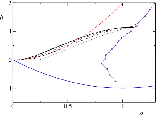
The DNLS dynamics are characterized by two conserved quantities: the energy densityhand the mass densitya(also termed norm—see the following section for their definitions). Therefore, a generic thermodynamic state of the DNLS equation can be seen as a point in the(a,h)plane. The equilibrium thermodynamics of the DNLS model was studied in a seminal paper by Rasmussen et al. [11] within the grand-canonical formalism. Here, it was shown that an equation of state can be formally derived with the help of transfer–integral techniques. Accordingly, any thermodynamic equilibrium state(a,h) can be equivalently represented in terms of a temperatureTand a chemical potentialµwhich can be
numerically determined by implementing suitable microcanonical definitions [12,13]. In Reference [11], it was found that a line of infinite–temperature equilibrium states in the(a,h)plane separates standard thermodynamic states, characterized by a positiveT, from those characterized by negative absolute temperatures. The existence of negative temperatures can be traced back to the properties of the two conserved quantities of the system. From the point of view of dynamics, it was realized that negative temperatures can be associated to the presence of intrinsically localized excitations, named discrete breathers (DB) (see e.g., [14–16]). In a series of important papers, Rumpf developed entropy-based arguments to describe the asymptotic states above this infinite-temperature line [17–20]. It has been later found that negative–temperature states can form spontaneously via the dynamics of the DNLS equation. They persist over extremely long time scales, that might grow exponentially with system size as a result of an effective mechanism of ergodicity–breaking [21].
A related question is whether the dynamics of the system influences non-equilibrium properties when the system exchanges energy and/or mass with the environment. In a series of papers [21–23], it has been found that when pure dissipators act at both edges of a DNLS chain (a case sometimes called boundary cooling [24–27]) the typical final state consists of an isolated static breather embedded in an almost empty background. The breather collects a sensible fraction of the initial energy and it is essentially decoupled from the rest of the chain. The spontaneous creation of localized energy spots out of fluctuations has further consequences on the relaxation to equipartition, since the interaction with the remaining part of the chain can become exponentially weak [28,29]. A similar phenomenon occurs after a quench from high to low temperatures in oscillator lattices [30]. Also, boundary driving by external forces may induce non-linear localization [31–33].
When, instead, the chain is put in contact with thermal baths at its edges, non-equilibrium stationary states characterized by a gradient of temperature and chemical potential emerge [13]. Local equilibrium is typically satisfied so that the overall state of the chain can be conveniently represented as a path in the(a,h)plane connecting two points corresponding to the thermodynamic variables imposed by the two reservoirs. The associated transport of mass and energy is typically normal (diffusive) and can be described in terms of the Onsager formalism. However, peculiar features, such as non-monotonous temperature profiles [34] or persistent currents [35], are found as well as a signature of anomalous transport in the low-temperature regime [36,37].
In this paper we consider a set-up where one edge is in contact with a heat reservoir at temperature TL and chemical potential µL, while the other interacts with a pure dissipator, i.e., a mass sink.
The original motivation for studying this configuration was to better understand the role of DBs in thermodynamic conditions. At variance with standard set-ups [1,2], this is conceptually closer to a semi-infinite array in contact with a single reservoir. In fact, on the pure-dissipator side, mass can only flow out of the system.
The presence of a pure dissipator forces the corresponding path to terminate close to the point (a=0,h=0), which is singular both inTandµ. This is indeed the point where the infinite- and the
zero-temperature lines collapse. Therefore, slight deviations may easily lead to crossing theβ =0
line, whereβ=1/Tis the inverse temperature. This is indeed the typical scenario observed for small TL, whenβsmoothly changes sign twice before approaching the dissipator (see Figure1for a few
sampled paths). The size of the negative-temperature region increases withTLand appears to be stable
over long time scales. Upon further increasingTL, a different stationary regime is found, characterized
extends up to the dissipator edge and then it progressively shrinks in favour of a positive-temperature region (on the other side of the chain). In this regime, the dynamics are controlled by the spontaneous formation (birth) and disappearance (death) of discrete breathers.
0 0.5 1
a
-1 0 1 2
[image:3.595.171.426.140.329.2]h
Figure 1.Phase diagram of the DNLS equation in the (a−h) plane of, respectively, energy and mass densities. The positive-temperature region extends between the ground stateβ= +∞line (solid blue
lower curve) and theβ=0 isothermal (red dashed curve). Purple circles show theµ=0 line, which
has been determined numerically through equilibrium simulations (data are taken from Reference [13]). Black curves refer to nonequilibrium profiles obtained by employing a heat bath with parameters TL=3 andµL=0 and a pure dissipator located at the left and right edges of the chain, respectively. Dotted, dot-dashed, dot-dot-dashed and solid curves refer to chain sizesN =511, 1023, 2047, and 4095, respectively. Upon increasingN, these above profiles tend to enter the negative temperature region. Simulations are performed by evolving the DNLS chain over 107time units after a transient of 4×10⁷units. For the system sizeN =4095, a further average over 10 independent trajectories is performed.
In Section2we introduce the model and briefly recall the definition of the main observables. Section 3 is devoted to a detailed characterization of the low-temperature phase, while the far-from-equilibrium phase observed for large TL is discussed in Section4. This is followed by
the analysis of the statistical properties of the birth/death process of large-amplitude DBs, illustrated in Section5. Finally, in Section 6we summarize the main results and comment about possible relationships with similar phenomena previously reported in the literature.
2. Model and Methods
We consider a DNLS chain of sizeNand with open boundary conditions, whose bulk dynamics is ruled by the equation
iz˙n =−2|zn|2zn−zn−1−zn+1 (1) where (n=1, . . . ,N) andzn= (pn+iqn)/
√
2 are complex variables, withqnandpnbeing standard
conjugate canonical variables. The quantityan =|zn(t)|2can be interpreted as thenumber of particles,
or, equivalently, themassin the lattice sitenat timet. Upon identifying the set of canonical variables znandiz∗n, Equation (1) can be read as the equation of motion generated by the Hamiltonian functional
H=
N
∑
n=1
|zn|4+z∗nzn+1+znz∗n+1
through the Hamilton equations ˙zn =−∂H/∂(iz∗n). We are dealing with a dimensionless version of
the DNLS equation: the nonlinear coupling constant and the hopping parameters, which are usually indicated explicitly in the Hamiltonian (2), have been set equal to unity. Accordingly, also the time variabletis expressed in arbitrary adimensional units. Without loss of generality, this formulation has the advantage of simplifying numerical simulations.
A relevant property of the DNLS dynamics is the existence of a second conserved quantity beside the total energyH, namely the total mass
A=
N
∑
n=1
|zn|2. (3)
As a result, an equilibrium state is specified by two parameters, the mass densitya=A/N≥0 and the energy densityh= H/N. The first reconstruction of the equilibrium phase-diagram(a,h)of the DNLS equation was reported in [11]. It is reproduced in Figure1for our choice of parameters, where the lower solid line defines the(T=0)ground-state lineh=a2−2afor different values of the mass densitya. The ground-state corresponds to a uniform state with constant amplitude and constant phase-differenceszn =
√
aei(µt+πn), withµ = 2(a−1). States below this curve are not physically
accessible. The positive-temperature region lies above the ground-state up to the red dashed line h=2a2, which corresponds to the infinite-temperature(β=0)line. In this limit, the grand-canonical
equilibrium distribution becomes proportional to exp(βµA), where the finite (negative) product βµimplies a diverging chemical potential. Equilibrium states at infinite temperature are therefore
characterized by an exponential distribution of the amplitudesP(|zn|2) =a−1e−|zn|
2/a
and random phases. Finally, states above theβ=0 line belong to the so-called negative-temperature region [11,21].
Finite-temperature equilibrium states do not allow for straightforward analytical treatments. However, one can determine the relation a(T,µ), h(T,µ) numerically, by putting the system
in interaction with an external reservoir (see below) that imposes T and µ and by measuring
the corresponding equilibrium densities. This method was adopted in Reference [13] to identify theµ=0
line shown in Figure1. Upon increasingµ, the curve moves to the right in the(a,h)diagram and becomes
more and more vertical (data not shown). Isothermal linesT=ccan be found analogously: they roughly follow the profile of theT = 0 line and, upon increasingc, they span all the positive-temperature region, approaching the infinite-temperature line forc→+∞[13].
A non-equilibrium steady state can be represented as a path in the (a,h)-parameter space, wherea(x)is the mass density,h(x)the energy density, andx = n/Nthe rescaled position along the chain. In our set-up, the first site of the chain (n=1) is in contact with a reservoir at temperature TLand chemical potentialµL. This is ensured by implementing the non-conservative Monte-Carlo
dynamics described in Reference [13]. In a few words, the reservoir performs random perturbations
δz1 = (δp1 +iδq1)/ √
2 of the state variable z1 that are accepted or rejected according to a grand-canonical Metropolis cost-function exp[−TL(∆H−µL∆A)], where∆Hand∆Aare respectively
the variations of energy and mass produced by δz1. The perturbations δp1 and δq1 are independent random variables extracted from a uniform distribution in the interval [−R,R]. The opposite site (n=N) interacts with a purestochastic dissipatorthat sets the variablezNequal to zero,
thus absorbing an amount of mass equal to|zN|2. Both the heat bath and the dissipator are activated
at random times, whose separations are independent and identically distributed variables uniformly distributed within the interval[tmin,tmax]. On average, this corresponds to simulating an interaction
process with decay rate γ ∼ ¯t−1, where ¯t = (tmax+tmin)/2. Notice that different prescriptions,
Throughout the paper we deal with measurements of temperature profiles. Since the DNLS Hamiltonian is not separable, the standard relation between temperature and local kinetic energy does not hold. Due to the existence of the second conserved quantityA, it is necessary to make use of the microcanonical definition provided in [39] and further extended in [12]. Its derivation is founded on the thermodynamic relation
β=T−1= ∂S ∂E
A=M (4)
for a system with total energyH=E, total massA=Mand entropyS. The calculation amounts to derive a measure of the hyper-surface at constant energy and mass in the phase space and to compute its variation with respect toEat constant mass. The general expression ofTis a thermal average of a non-local function of the dynamical variablesznandz∗nand is rather involved; we refer to [13,21]
and the related bibliography for theoretical and computational details.
In what follows, we consider a situation where all parameters, other thanTL, are kept fixed.
In particular, we have chosenµL=0,R=0.8 and ¯t=3×10⁻², withtmaxandtminof order 10−2. We have
verified that the results obtained for this choice of the parameter values are general. A more detailed account of the dependence of the results on the thermostat properties will be reported elsewhere.
Finally, we recall the observables that are typically used to characterize a steady-state out of equilibrium: the mass flux
ja=2hIm(zn∗zn+1)i, (5)
and the energy flux
jh=2hRe(z˙nz∗n+1)i, (6)
where the angular brackets denote a time average.
3. Low-Temperature Regime: Coupled Transport and Negative Temperatures
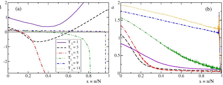
In the left panel of Figure2, we report the average profile of the inverse temperature β(x)
as a function of the rescaled site position x = n/N, for different values of the temperature of the thermostat. A first “anomaly” is already noticeable for relatively small TL: the profile is
non monotonous (see for example the curve forTL = 1). This feature is frequently encountered
when a second quantity, besides energy, is transported [13,40,41]. In the present setup, this second thermodynamic observable is the chemical potentialµ(x), set equal to zero at the left edge. Rather than
plottingµ(x), in the right panel of Figure2, we have preferred to plot the more intuitive mass density a(x). There we see that the profile forTL=1 deviates substantially from a straight line, indicating that
the thermodynamic properties vary significantly along the chain and suggesting that the lattice might not be long enough to ensure an asymptotic behavior.
To clarify this point, we have performed simulations for different values of N. The results for TL = 1 are reported in Figure 3, where we plot the local temperature T as a function of x.
All profiles start fromT=1, the value imposed by the thermostat and, after an intermediate bump, eventually attain very small values. Since neither the temperature nor the chemical potential are directly imposed by the purely dissipating “thermostat”, it is not obvious to predict the asymptotic value of the temperature (and the chemical potential). The data reported in the inset suggest a sort of logarithmic growth withN, but this is not entirely consistent with the results obtained forTL=3
(see below).
If transport were normal andNwere large enough, the various profiles should collapse onto each other, but this is far from the case displayed in Figure 3. The main reason for the lack of convergence is the growth of the temperature bump. This is because, upon further increases ofN, the system spontaneously crosses the infinite temperature line and enters the negative-temperature region. ForTL=3, this “transition” has already occurred forN=4095, as it can be seen in Figure2.
The crossings of the infinite temperature points (β=0) at the boundaries of the negative temperature
productβµremains finite at these turning points (data not reported). To our knowledge, this is the
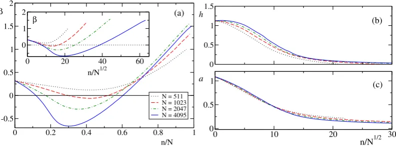
first example of negative-temperature states robustly obtained and maintained in nonequilibrium conditions in a chain coupled with a single reservoir at positive temperature. In order to shed light on the thermodynamic limit, we have performed further simulations for different system sizes. In Figure4, we report the results obtained forTL =3 andNranging from 511 to 4095. In Figure4a, we see that the
negative-temperature region is already entered forN=1023. Furthermore, its extension grows with N, suggesting that in the thermodynamic limit it would cover the entire profile but the edges.
Since non-extensive stationary profiles have been previously observed both in a DNLS and a rotor chain (i.e., the XY-model ind = 1) at zero temperature and in the presence of chemical potential gradients [42], it is tempting to test to what extent an anomalous scaling (sayn/√N) can account for the observations. In the inset of Figure4a, we have rescaled the position along the lattice by√N. For relatively small but increasing values ofn/√Nwe do see a convergence towards an asymptotic curve, which smoothly crosses theβ = 0 line. This suggests that close to the left edge, positive
temperatures extend over a range of order O(√N), thereby covering a non-extensive fraction of the chain length. The scaling behavior in the rest of the chain is less clear, but it is possibly a standard extensive dynamics characterized by a finite temperature on the right edge. A confirmation of the anomalous scaling in the left part of the chain is obtained by plotting the profiles ofhandaagain as a function ofn/√N(see the panels (b) and(c) in Figure4, respectively). Further information can be extracted from the scaling behavior of the stationary mass fluxja. In Figure5, we report the average
value ofjaas a function of the lattice length. There, we see thatjadecreases roughly asN−1/2. At a
[image:6.595.87.512.396.558.2]first glance this might be interpreted as a signature of energy super-diffusion, but it is more likely due to the presence of a pure dissipation on the right edge (in analogy to what seen in the XY-model [43]).
Figure 2.Average profiles of the inverse temperatureβ(x)(panel (a)) and mass-densitya(x)(panel (b))
for a DNLS chain withN =4095 and different temperaturesTLof the reservoir acting at the left edge, whereµ = 0. The profileβ(x)is computed making use of the microcanonical definition of
0 0.2 0.4 0.6 0.8 1 x = n/N
0 1 2 3 T(x)
N = 511 N = 1023 N = 2047 N = 4095
102 103 N
[image:7.595.185.410.86.252.2]-4 0 4 βR,µR
Figure 3.Average profiles of the temperatureT(x)forTL=1 and different system sizesN. The profile
T(x)is computed by means of the microcanonical definition of temperature. The inset shows the boundary inverse temperatureβR(black circles) and chemical potentialµR(red squares) close to the dissipator side as a function of the system sizeN. The data refers to the microcanonical definitions of temperature and chemical potential computed on the last 10 sites of the chain. Simulations are performed evolving the system over 107time units after a transient of 4×10⁷units. For the system sizeN=4095 a further average over 10 independent trajectories has been performed.
0 0.2 0.4 0.6 0.8 1
n/N -0.5
0 0.5 1 1.5 2
β
N = 511 N = 1023 N = 2047 N = 4095
0 20 40 60
n/N1/2 0
1 2
β (a)
0 0.5 1 1.5 h
0 10 20 30
n/N1/2
0 0.5 1
a
(b)
(c)
Figure 4.Panel (a): average profiles of inverse temperatureβforTL=3 and different system sizes
N. The profileβis computed by means of the microcanonical definition of temperature. In the inset,
[image:7.595.100.497.372.520.2]10
3N
10
410
-410
-310
-210
-1j
aTL= 1 TL= 3 TL = 9 TL = 11
0
5
10
T
L
10
-410
-310
-2j
[image:8.595.172.421.85.265.2]a
Figure 5.Average mass fluxjaversus system sizeNfor different reservoir temperaturesTL. The black dotted line refers to a power-law decayja ∼ N−1/2. The inset shows the dependence of ja on the reservoir temperatureTLfor the system size N = 4095. Simulations are performed evolving the DNLS chain over 107time units after a transient of 4×10⁷units. For the system sizeN=4095 we have averaged over 10 independent trajectories.
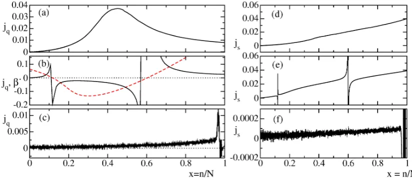
In stationary conditions, mass, and energy fluxes are constant along the chain. This is not necessarily true for the heat flux, as it refers only to the incoherent component of the energy transported across the chain. More precisely, the heat flux is defined asjq(x) = jh−jaµ(x)[43] Sincejaandjh
are constant, the profile of the heat flux jq is essentially the same of theµ profile (up to a linear
transformation). In Figure6a, we report the heat flux forTL=1. It is similar to the temperature profile
displayed in Figure3. It is not a surprise to discover thatjqis larger where the temperature is higher.
Figure6b in the same Figure6refers toTL=3. A very strange shape is found: the flux does not only
changes sign twice but exhibits a singular behavior in correspondence of the change of sign, as if a sink and source of heat were present in these two points, where the chemical potential and the local temperature diverge (see, e.g., the red dashed line in Figure6b representing theβprofile). The scenario
looks less awkward if the entropy fluxjs = jq/T is monitored. ForTL = 1, the bump disappears
and we are in the presence of a more “natural” shape (see Figure6d) More important is to note that the singularities displayed byjqforTL =3 are almost removed since they occur whereT→∞(we are
convinced that the residual peaks are due to a non perfect identification of the singularities). If one removed the singular points, the profile of the entropy fluxjs= jq/Thas a similar shape for the cases TL=1 andTL=3. A more detailed analysis of the scenario is, however, necessary in order to provide
Figure 6. Profiles of heat flux (black lines) forTL = 1 (panel (a)),TL = 3 (panel (b)) andTL = 9 (panel (c)) in a chain withN=4095 lattice sites. For each boundary temperature, we find the following values of mass and energy fluxes: panel (a)ja=3.5×10⁻³,jh=−3.3×10⁻⁴; panel (b)ja=2.5×10⁻³,
jh=3.4×10⁻⁴; panel (c)ja=1.2×10⁻⁴,jh=1.5×10⁻⁴. The red dashed line in panel (b) refers to the rescaled profile of the inverse temperatureβ0(x) =β(x)/5 measured along the chain (see Figure2).
Panels (d–f) show the profiles of entropy flux for the same temperatures:TL=1,TL=3 andTL=9, respectively. Other simulation details are the same as given in Figure2.
4. High Temperature Regime: DB Dominated Transport
Let us now turn our attention to the high-temperature case. As shown in Figure2a, for sufficiently largeTL values, the positive-temperature region close to the dissipator disappears (this is already
true forTL =5) and, at the same time, the positive-temperature region on the left grows. In other
words, negative temperatures are eventually restricted to a tiny region close to the dissipator side. This stationary state is induced by the spontaneous formation and the destruction of large DBs close to the dissipator. On average, such a process gives rise to locally steep amplitude profiles that are reminiscent of barriers raised close to the right edge of the chain, see Figure2b. As it is well known, DBs are localized nonlinear excitations typical of the DNLS chain. Their phenomenology has been widely described in a series of papers where it has been shown that they emerge when energy is dissipated from the boundaries of a DNLS chain [21–23]. In fact, when pure dissipators act at both chain boundaries, the final state turns out to be an isolated DB embedded in an almost empty background. In view of its localized structure and the fast rotation, the DB is essentially uncoupled from the rest of the chain and, a fortiori, from the dissipators. One cannot exclude that a large fluctuation might eventually destroy the DB, but this would be an extremely rare event.
In the setup considered in this paper, DB formation is observed in spite of one of the two dissipators being replaced by a reservoir at finite temperature. DBs are spontaneously produced close to the dissipator edge only for sufficiently high values ofTL. Due to its intrinsic nonlinear character,
spot DBs simply by looking at the average mass profiles. In Figure2, the presence of a DB is signaled by the sharp peak close to the right edge for bothTL=9 andTL =11.
The region between the reservoir and the DB should, in principle, evolve towards an equilibrium state at temperatureTL. However, a close look at theβ-profile in Figure2reveals the presence of
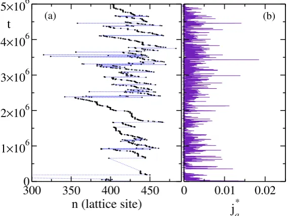
a moderate temperature gradient that is typical of a stationary non-equilibrium state. In fact, DBs are not only born out of fluctuations, but can also collapse due to local energy fluctuations. As shown in Figure7a, once a DB is formed, it tends to propagate towards the heat reservoir located at the opposite edge. The DB position is tagged by black dots drawn at fixed time intervals over a very long time lapse ofO(106), in natural time units of the model. This backward drift comes to a “sudden” end when a suitable energy fluctuation destroys the DB (see Figure7a). Afterwards, mass and energy start flowing again towards the dissipator, until a new DB is spontaneously formed by a sufficiently large fluctuation close to the dissipator edge (the formation of the DB is signaled by the rightmost black dots in Figure7a) and the conduction of mass and energy is inhibited again. The DB lifetime is rather stochastic, thus yielding a highly irregular evolution. The statistical properties of such birth/death process are discussed in the following section.
300
350
400
450
n (lattice site)
0
1
×
10
62
×
10
63
×
10
64
×
10
65
×
10
6t
0
0.01
0.02
j
a* [image:10.595.156.443.306.520.2](a) (b)
Figure 7.(a) Qualitative DB trajectory in a stationary state withN=511 andTL=10. Each point of the curve corresponds to the position of the maximum average amplitude of the chain in a temporal window of 5×10³time units. (b) Temporal evolution of the outgoing mass fluxj∗athrough the dissipator edge during the same dynamics of panel (a). The fluxj∗ais computed every 20 time units as the average amount of mass flowing to the dissipator during such time interval. Higher peaks typically correspond to the breakdown of one or more DBs. Notice that the boundary mass flux can take only positive values because the chain interacts with a pure dissipator.
The statistical process describing the appearance/disappearance of the DB is a complex one. On the one hand, we are in the presence of a stationary regime: the mass and energy currents flowing through the dissipator are found to be constant, when averaged over time intervals much longer than the typical DB lifetime. On the other hand, strong fluctuations in the DB lifetime mean that this regime is not steady but it rather corresponds to a sequence of many different macrostates, some of which are likely to be far from equilibrium. Altogether, in this phase, the presence of long lasting DBs induces a substantial decrease of heat and mass conduction. This is clearly seen in Figure5, wherejais plotted
for different chain lengths. The two set of data corresponding toTL =9 and 11 are at least one order of
two conduction regimes is neatly highlighted in the inset of Figure5, where the stationary mass flux is reported as a function of the reservoir temperature for the sizeN=4095.
The effect of the appearance and disappearance of the DB in the high reservoir temperature regime on the transport of heat and mass along the chain is twofold. During the fast dynamics, it produces bursts in the output fluxes of these quantities as demonstrated in Figure7b. When the DB is present the boundary flux to the dissipator decreases, while when the DB disappears, avalanches of heat and mass reach the dissipator. In the slow dynamics obtained by averaging over many bursts, the conduction of heat and mass from the heat reservoir to the dissipator is hugely reduced with respect to the low temperature regime. We can conclude that the most important effect of the intermittent DB in the high temperature regime is to act as a thermal wall.
Finally, in Figure6c,f we plot the heat and entropy profiles observed in the high-temperature phase, respectively. The strong fluctuations in the profiles are a consequence of the large fluctuations in the DB birth/death events and its motion. It is now necessary to average over much longer time scales to obtain sufficiently smooth profiles. It is interesting, however, to observe that the profile ofjs in Figure6f exhibits an overall shape similar to that observed in the low temperature regimes
(see Figure6d,e). This notwithstanding, there are two main differences with the low temperature behavior. First, close to the right edge of the dissipator we are now in presence of wild fluctuations of js, and second the overall scale of the entropy flux profile is heavily reduced.
5. Statistical Analysis
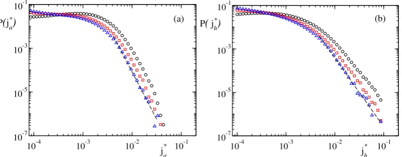
In order to gain information on the high-temperature regime, it is convenient to look at the fluctuations of the boundary mass flux j∗a and the boundary energy flux j∗h flowing through
the dissipator edge. In Figure8we plot the distribution of bothja∗(panel (a)) andjh∗(panel (b)) for TL=11 for different chain lengths. In both cases, power-law tails almost independent ofNare clearly
visible. This scenario is highly reminiscent of the avalanches occurring in sandpile models. In fact, one such analogy has been previously invoked in the context of DNLS dynamics to characterize the atom leakage from dissipative optical lattices [44].
10-4 10-3 10-2 10-1
ja*
10-7 10-5 10-3 10-1
P(ja*
)
(a)10-4 10-3 10-2 10-1 jh* 10-7
10-5 10-3 10-1
[image:11.595.101.500.462.618.2]P
(
jh*)
(b)Figure 8.Normalized boundary flux distributions through the dissipator for a stationary state with TL=11. Panel (a) shows the mass flux distributionP(j∗a), while panel (b) refers to the energy flux distributionP j∗h
. Black circles, red squares, and blue triangles refer to system sizesN=511, 1023, and 2047, respectively. Power-law fits on the largest sizeN = 2047 (see black dashed lines) give P(j∗a) ∼j∗a−4.32andP(j∗h) ∼j∗h−3.17. Boundary fluxes are sampled by evolving the DNLS chain for a total timetf after a transient of 4×10⁷ temporal units and averaged over time windows of five temporal units. For the sizesN = 511 andN =1023 we have considered a single trajectory with tf =108. For the sizeN=2047 the distributions are extracted from five independent trajectories with
We processed the time series of the type reported in Figure7b to determine the durationτb of
the bursts (avalanches) andτlof the “laminar” periods in between consecutive bursts (i.e., the DB
life-times). In practice, we have first fixed a flux threshold (s=4.25×10⁻³) to distinguish between burst and laminar periods. Furthermore, a series of bursts separated by a time shorter thandt0=103 has been treated as a single burst. This algorithm has been applied to 20 independent realizations of the DNLS dynamics in the high-temperature regime. Each realization has been obtained by simulating a lattice withN=511 sites,TL=10, and for a total integration timet=5×10⁶. In these conditions
we have recorded nearly 7000 avalanches.
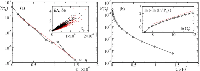
The probability distribution of the burst duration is plotted in Figure9a. It follows a a Poissonian distribution, typical of random uncorrelated events. We have also calculated the amount of mass Aand energyEassociated with each burst, integrating mass, and energy fluxes during each burst. The results are shown as a scatter plot in the inset of Figure9a. They display a clear (and unsurprising) correlation between these two quantities.
0 0.5 1 1.5 2
τ
b ×10 4 10-7 10-6 10-5 10-4 10-3 P(τ b)
0 1×10⁴
2×10⁴
τ
b
0 2 4 δA, δE (a)
0 0.5 1 1.5 2
τ l×10
5 10-8 10-7 10-6 10-5 10-4 10-3 P(τ l)
8 10 12
ln (τ
l)
0 1 2 3
ln (- ln (P / P
[image:12.595.100.498.277.419.2]0) ) (b)
Figure 9. (a) Probability distribution of the duration of burstsτb. Note the logarithmic scale on the vertical axis. From an exponential fitP ∼ e−γτb, we find a decay constantγ = 5×10⁻⁴ (red dashed line). The inset shows the relation between the durationτband the amount of massδA(black
dots) and energyδE(red dots) released to the dissipator. (b) Probability distribution of DB lifetimes.
In the inset we show that this is compatible with a stretched exponential lawP=P0e−τσ
l, whereσ'0.5 (red dashed line) andP0is the maximum value of the distribution.
The time interval between two consecutive bursts is characterized by a small mass flux. Typically, during this period the chain develops a stable DB that inhibits the transfer of mass towards the dissipator. Figure9b shows the probability distribution of the duration of these laminar periods. The distribution displays a stretched-exponential decay with a characteristic constantσ=0.5.
Such a scenario is consistent with the results obtained in [26] for the Fermi-Pasta-Ulam chain and in [22] for the DNLS lattice. The values of the powerσfound in these papers are not far from the one
that we have obtained here (see also [45] for similar results on rotor models).
6. Conclusions
We have investigated the behavior of a discrete nonlinear Schrödinger equation sandwiched between a heat reservoir and a mass/energy dissipator. Two different regimes have been identified upon changing the temperature TL of the heat reservoir, while keeping fixed the properties of
the dissipator. For low TL and low chemical potential, a smooth β-profile is observed, which
extends (in the central part) to negative temperatures without, however, being accompanied by the formation of discrete breathers over the time scales accessible to numerical simulations. In the light of the theoretical achievements by Rumpf [17–20], the negative-temperature regions are incompatible with the assumption of local thermodynamic equilibrium, which instead appears to be satisfied in the positive-temperature part. Therefore, despite the smoothness of the profiles and the stationarity of mass and energy fluxes, such negative-temperature configurations should be better considered as metastable states. Unfortunately, it is not easy to investigate this regime; no single heat bath can impose a fixed negativeTin a meaningful way so as to be able to compare with equilibrium states. It is therefore necessary to simulate larger systems in the hope to observe the spontaneous formation of breathers, the only obvious signature of negative temperatures. We plan to undertake such a kind of numerical studies in the near future. It is nevertheless remarkable to see that negative temperatures are steadily sustained for moderately long chain lengths. As a second anomaly, we report the slow decrease of the mass-flux with the chain length: the hallmark of an unconventional type of transport. This feature is, however, not entirely new; a similar scenario has been previously observed in setups with dissipative boundary conditions and no fluctuations [42].
For larger temperaturesTL, we observe an intermittent regime characterized by the alternation of
insulating and conducting states, triggered by the appearance/disappearance of discrete breathers. Note that this regime is rather unusual, since it is generated by increasing the amount of energy provided by the heat bath rather than by decreasing the chemical potential, as observed for example in the superfluid/Mott insulator transition in Bose-Einstein condensates in optical lattices. Although, for clarity, we referred to the low and highTLcases, there is no special difference to be expected in the
intermediate regime, except for the typical timescale for DB creation that may be, still, exceedingly large. In fact, for finiteN, such a timescale becomes much shorter above some typicalTL.
The intermittent presence of a DB/wall makes the chain to behave as ararely leaking pipe, which releases mass droplets at random times when the DB disappears according to a stretched-exponential distribution. The resulting fluctuations of the fluxes suggest that the regime is stationary but not steady, i.e., locally the chain irregularly oscillates among different macroscopic states characterized, at best, by different values of the thermodynamic variables. A similar scenario is encountered in the XY chain, when both reservoirs are characterized by a purely dissipation accompanied by a deterministic forcing [42]. In such a setup, as discussed in Reference [42], the temperature in the middle of the chain fluctuates over macroscopic scales. Here, however, given the rapidity of changes induced by the DB dynamics, there may be no well-defined values of the thermodynamic observables. For example, during an avalanche it is unlikely that temperature and chemical potentials are well-defined quantities, as there may not even be a local equilibrium. This extremely anomalous behavior is likely to smear out in the thermodynamic limit, since the breather life-time does not probably increase with the system size, however, it is definitely clear that the associated fluctuations strongly affect moderately-long DNLS chains.
Acknowledgments: This research did not receive any funding. Stefano Lepri acknowledges hospitality of the Institut Henri Poincaré-Centre Emile Borel during the trimester Stochastic Dynamics Out of Equilibrium where part of this work was elaborated.
Author Contributions: Stefano Iubini performed the numerical simulations. All Authors contributed to the research work and to writing the paper.
Abbreviations
The following abbreviations are used in this manuscript:
DNLS Discrete Nonlinear Schrödinger DB Discrete Breather
References
1. Lepri, S.; Livi, R.; Politi, A. Thermal conduction in classical low-dimensional lattices. Phys. Rep.2003, 377, 1–80.
2. Dhar, A. Heat Transport in low-dimensional systems.Adv. Phys.2008,57, 457–537.
3. Basile, G.; Delfini, L.; Lepri, S.; Livi, R.; Olla, S.; Politi, A. Anomalous transport and relaxation in classical one-dimensional models. Eur. Phys J. Spec. Top.2007,151, 85–93.
4. Eilbeck, J.C.; Lomdahl, P.S.; Scott, A.C. The discrete self-trapping equation. Physica D1985,16, 318–338. 5. Eilbeck, J.C.; Johansson, M. The Discrete Nonlinear Schrödinger Equation-20 Years on; World Scientific:
Singapore, 2003.
6. Kevrekidis, P.G.The Discrete Nonlinear Schrödinger Equation; Springer: Berlin/Heidelberg, Germany, 2009. 7. Scott, A.Nonlinear Science. Emergence and Dynamics of Coherent Structures; Oxford University Press: Oxford,
UK, 2003.
8. Kosevich, A.M.; Mamalui, M.A. Linear and nonlinear vibrations and waves in optical or acoustic superlattices (photonic or phonon crystals).J. Exp. Theor. Phys.2002,95, 777.
9. Hennig, D.; Tsironis, G. Wave transmission in nonlinear lattices. Phys. Rep.1999,307, 333–432.
10. Franzosi, R.; Livi, R.; Oppo, G.; Politi, A. Discrete breathers in Bose–Einstein condensates. Nonlinearity
2011,24, R89.
11. Rasmussen, K.; Cretegny, T.; Kevrekidis, P.G.; Grønbech-Jensen, N. Statistical mechanics of a discrete nonlinear system. Phys. Rev. Lett.2000,84, 3740–3743.
12. Franzosi, R. Microcanonical Entropy and Dynamical Measure of Temperature for Systems with Two First Integrals.J. Stat. Phys.2011,143, 824–830.
13. Iubini, S.; Lepri, S.; Politi, A. Nonequilibrium discrete nonlinear Schrödinger equation. Phys. Rev. E2012, 86, 011108.
14. Sievers, A.; Takeno, S. Intrinsic localized modes in anharmonic crystals. Phys. Rev. Lett.1988,61, 970. 15. MacKay, R.; Aubry, S. Proof of existence of breathers for time-reversible or Hamiltonian networks of
weakly coupled oscillators. Nonlinearity1994,7, 1623.
16. Flach, S.; Gorbach, A.V. Discrete breathers—Advances in theory and applications. Phys. Rep.2008,467, 1–116. 17. Rumpf, B. Simple statistical explanation for the localization of energy in nonlinear lattices with two
conserved quantities.Phys. Rev. E2004,69, 016618.
18. Rumpf, B. Transition behavior of the discrete nonlinear Schrödinger equation.Phys. Rev. E2008,77, 036606. 19. Rumpf, B. Stable and metastable states and the formation and destruction of breathers in the discrete
nonlinear Schrödinger equation. Phys. D Nonlinear Phenom.2009,238, 2067–2077.
20. Rumpf, B. Growth and erosion of a discrete breather interacting with Rayleigh-Jeans distributed phonons. Europhys. Lett.2007,78, 26001.
21. Iubini, S.; Franzosi, R.; Livi, R.; Oppo, G.; Politi, A. Discrete breathers and negative-temperature states. New J. Phys.2013,15, 023032.
22. Livi, R.; Franzosi, R.; Oppo, G.L. Self-localization of Bose-Einstein condensates in optical lattices via boundary dissipation. Phys. Rev. Lett.2006,97, 60401.
23. Franzosi, R.; Livi, R.; Oppo, G.L. Probing the dynamics of Bose–Einstein condensates via boundary dissipation. J. Phys. B At. Mol. Opt. Phys.2007,40, 1195.
24. Tsironis, G.; Aubry, S. Slow relaxation phenomena induced by breathers in nonlinear lattices.Phys. Rev. Lett.
1996,77, 5225.
25. Piazza, F.; Lepri, S.; Livi, R. Slow energy relaxation and localization in 1D lattices. J. Phys. A Math. Gen.
2001,34, 9803.
27. Reigada, R.; Sarmiento, A.; Lindenberg, K. Breathers and thermal relaxation in Fermi–Pasta–Ulam arrays. Chaos2003,13, 646–656.
28. De Roeck, W.; Huveneers, F. Asymptotic localization of energy in nondisordered oscillator chains. Commun. Pure Appl. Math.2015,68, 1532–1568.
29. Cuneo, N.; Eckmann, J.P. Non-equilibrium steady states for chains of four rotors.Commun. Math. Phys.
2016,345, 185–221.
30. Oikonomou, T.; Nergis, A.; Lazarides, N.; Tsironis, G. Stochastic metastability by spontaneous localisation. Chaos Solitons Fractals2014,69, 228–232.
31. Geniet, F.; Leon, J. Energy transmission in the forbidden band gap of a nonlinear chain. Phys. Rev. Lett.
2002,89, 134102.
32. Maniadis, P.; Kopidakis, G.; Aubry, S. Energy dissipation threshold and self-induced transparency in systems with discrete breathers.Phys. D Nonlinear Phenom.2006,216, 121–135.
33. Johansson, M.; Kopidakis, G.; Lepri, S.; Aubry, S. Transmission thresholds in time-periodically driven nonlinear disordered systems. Europhys. Lett.2009,86, 10009.
34. Iubini, S.; Lepri, S.; Livi, R.; Politi, A. Off-equilibrium Langevin dynamics of the discrete nonlinear Schroedinger chain. J. Stat. Mech Theory Exp.2013,2013, P08017 .
35. Borlenghi, S.; Iubini, S.; Lepri, S.; Chico, J.; Bergqvist, L.; Delin, A.; Fransson, J. Energy and magnetization transport in nonequilibrium macrospin systems. Phys. Rev. E2015,92, 012116.
36. Kulkarni, M.; Huse, D.A.; Spohn, H. Fluctuating hydrodynamics for a discrete Gross-Pitaevskii equation: Mapping onto the Kardar-Parisi-Zhang universality class. Phys. Rev. A2015,92, 043612.
37. Mendl, C.B.; Spohn, H. Low temperature dynamics of the one-dimensional discrete nonlinear Schroedinger equation.J. Stat. Mech Theory Exp.2015,2015, P08028.
38. Yoshida, H. Construction of higher order symplectic integrators. Phys. Lett. A1990,150, 262–268. 39. Rugh, H.H. Dynamical approach to temperature. Phys. Rev. Lett.1997,78, 772.
40. Iacobucci, A.; Legoll, F.; Olla, S.; Stoltz, G. Negative thermal conductivity of chains of rotors with mechanical forcing. Phys. Rev. E2011,84, 061108.
41. Ke, P.; Zheng, Z.G. Dynamics of rotator chain with dissipative boundary. Front. Phys.2014,9, 511–518. 42. Iubini, S.; Lepri, S.; Livi, R.; Politi, A. Boundary-induced instabilities in coupled oscillators. Phys. Rev. Lett.
2014,112, 134101.
43. Iubini, S.; Lepri, S.; Livi, R.; Politi, A. Coupled transport in rotor models. New J. Phys.2016,18, 083023. 44. Ng, G.; Hennig, H.; Fleischmann, R.; Kottos, T.; Geisel, T. Avalanches of Bose–Einstein condensates in
leaking optical lattices.New J. Phys.2009,11, 073045.
45. Eleftheriou, M.; Lepri, S.; Livi, R.; Piazza, F. Stretched-exponential relaxation in arrays of coupled rotators. Phys. D Nonlinear Phenom.2005,204, 230–239.
c