Evolutionary star-structured heterogeneous data co-clustering

(1)

Rochester Institute of Technology

RIT Scholar Works

Theses Thesis/Dissertation Collections

11-1-2012

Evolutionary star-structured heterogeneous data

co-clustering

Amit Salunke

Follow this and additional works at:http://scholarworks.rit.edu/theses

This Thesis is brought to you for free and open access by the Thesis/Dissertation Collections at RIT Scholar Works. It has been accepted for inclusion in Theses by an authorized administrator of RIT Scholar Works. For more information, please [email protected].

Recommended Citation

(2)

Evolutionary Star-Structured Heterogeneous Data

Co-Clustering

by

Amit M. Salunke

A Thesis Submitted in Partial Fulfillment of the Requirements for the Degree of Master of Science in Computer Science

Supervised by

Dr. Manjeet Rege

Department of Computer Science

B. Thomas Golisano College of Computing and Information Sciences Rochester Institute of Technology

Rochester, New York November 2012

Approved By:

Dr. Manjeet Rege

Thesis Adviser, Department of Computer Science Primary Adviser

Dr. Xumin Liu

Committee Member, Department of Computer Science Reader

Dr. Aaron Deever

(3)

© Copyright 2012 by Amit M. Salunke

(4)

Abstract

A star-structured interrelationship, which is a more common type in real world data, has a

central object connected to the other types of objects. One of the key challenges in

evolu-tionary clustering is integration of historical data in current data. Traditionally, smoothness

in data transition over a period of time is achieved by means of cost functions defined

over historical and current data. These functions provide a tunable tolerance for shifts of

current data accounting instance to all historical information for corresponding instance.

Once historical data is integrated into current data using cost functions, co-clustering is

ob-tained using various co-clustering algorithms like spectral clustering, non-negative matrix

factorization, and information theory based clustering. Non-negative matrix factorization

has been proven efficient and scalable for large data and is less memory intensive

com-pared to other approaches. Non-negative matrix factorization tri-factorizes original data

matrix into row indicator matrix, column indicator matrix, and a matrix that provides

cor-relation between the row and column clusters. However, challenges in clustering evolving

heterogeneous data have never been addressed. In this thesis, I propose a new algorithm

for clustering a specific case of this problem, viz. the star-structured heterogeneous data.

The proposed algorithm will provide cost functions to integrate historical star-structured

heterogeneous data into current data. Then I will use non-negative matrix factorization to

cluster each time-step of instances and features. This contribution to the field will provide

(5)

List of Figures

2.1 The Star-Structured High-order Heterogeneous Data. . . 6

3.1 The Star-Structured Heterogeneous Data. . . 10

4.1 Image samples selected random from each image category . . . 20

4.2 Visualization of Synthetic data clustering over period of time from t0 to t7 : At time-step t1, Gaussian noise of 50 instances was added per cluster. At time-step t2 10 more instances were added from distribution of C2. At time-step t3 10 instances were removed from cluster C4. At time-step t5, 2 features were added to C4. 1 feature was removed from C1 at time-step t6. t7is unchanged from t6. . . 22

4.3 Comparison between accuracy of Evolutionary Higher order clustering(EHCC)

and Higher order Clustering(HCC) for Synthetic dataset . . . 23 4.4 Visualization of Synthetic data clustering over period of time from t0 to t7

:t0 is the original data. Between time steps t1 - t6, instances shown drift from C4to C5. Finally, at time step t7, 20 instances moved from C4to C5. . 24 4.5 Visualization of Synthetic data clustering over period of time from t0 to t7

:t0is the original data. Between time steps t1 - t6, features shown drift from C4to new cluster C6. At time step t5, 2 features moved from C4to C6. Over next few time steps, C6became more homogeneous. . . 25

and Higher order Clustering(HCC) for Web-service dataset . . . 26

and Higher order Clustering(HCC) for Text dataset,England-Heart,re0 . . 27

and Higher order Clustering(HCC) for Text dataset,Graft-Phos,re0 . . . . 27

and Higher order Clustering(HCC) for Text dataset,ArachidonicAcids-Hematocrit,

(8)

and Higher order Clustering(HCC) for Text dataset,Enzyme-Infections,re0 28

4.11 Comparison between evolutionary higher order clustering algorithm (EHCC) and Static Higher order clustering algorithm (HCC), and comparison of performances of evolutionary algorithm with respect to trade-of factorα . . 29 4.12 Change in number of clusters over period of time, for evolutionary higher

order clustering algorithm (EHCC) and Static Higher order clustering algo-rithm (HCC); and comparison of performances of evolutionary algoalgo-rithm with respect to trade-of factorα . . . 30 4.13 Number of instances in 5th cluster over period of time, for evolutionary

(9)

List of Tables

(10)

1. Introduction

Rapid development in data acquisition technology has resulted in the generation of large

amounts of raw data, providing significant potential for the development of automatic data

retrieval, analysis and mining. Data clustering is a well-known and widely used data mining

technique that groups data objects into different groups (known as clusters) based on a

predefined criterion of similarity [19] [20]. In other words, objects in a cluster are similar to

each other, while being dissimilar from the ones in a different cluster. Traditional clustering

methods perform one dimensional clustering, i.e. clustering of instances alone, and fail to

extract any information from the features [42].

Data co-clustering not only clusters instances and features together, but also extracts

relationships between instances and features being clustered [2] [10] [11] [13]. In general,

co-clustering problems involve two types of data that are pair-wise heterogenous in nature

and need to be clustered together. Dhillon [10] modeled the problem of co-clustering as a

graph partitioning problem. He performed co-clustering on words and documents dataset

using an singular value decomposition based algorithm to partition a bipartite graph

be-tweenword-document. Rege et al. [29] proposed an isoperimetric co-clustering algorithm

that is again a bipartite partitioning-based co-clustering model. Recently, it has been shown

that Non-negative Matrix Factorization (NMF) algorithms are less memory intensive and

outperform graph-based methods like spectral clustering (SVD) and iso-perimetric

co-clustering (ICA) in achieving higher accuracy and efficiency [24] [40] [7] [33].

In the real world, data types in domains such as multimedia [4], biomedicine [12] [28]

[41], and web mining [30] [39] are multi-type in nature. For example, Web images that are

generally surrounded by text describing the image can be clustered using their low-level

(11)

words and documents but fails to extract relations in higher-order heterogeneous data like

Web images. Rege et al. (CIHC) [31] and Gao et al. (CBGC) [15] modeled such problems

of heterogeneous data co-clustering as tripartite graph partitioning problems. Long et al.

[23] proposed a spectral clustering-based approach for higher-order heterogeneous data

co-clustering. Recently, non-negative matrix factorization has been used in order to perform

heterogeneous data co-clustering [7].

However, all of these efforts have been limited to static data. Data extracted from

cer-tain domains like social networks and web-blogs are evolving in nature. In these domains,

data collected over a short time interval exhibit high similarity over data instances and

fea-tures. This can be effectively used to optimize data clustering since changes in clustering

are gradual [6]. None of the algorithms discussed above take into account the passage of

time and knowledge that can be gained by observing data as it evolves. Chakrabarti et

al. [6] and Chi et al. [8] have shown that incorporation of historic knowledge improves

the clustering accuracy. Wang et al. [38] proposed that evolutionary clustering can be

effectively done by the amalgamation of low-rank matrix approximation methods and

ma-trix factorization-based clustering. Recently, Green et al. [16] proposed an evolutionary

spectral co-clustering approach for evolutionary data.

In the case of data extracted from domains like social networks and web blogs, the data

is heterogeneous as well as evolutionary. In spite of efforts on heterogeneous co-clustering

and evolutionary co-clustering algorithms, the problem of co-clustering-evolving-heterogeneous

data has not been addressed. To the best of my knowledge, there are no contributions

to-ward an algorithm that performs co-clustering on evolving heterogeneous data. In this

thesis, I propose a novel algorithm designed for co-clustering of evolving heterogeneous

data. The proposed algorithm is entitled EHCC (Evolutionary star-structured

Heteroge-neous Co-Clustering), which will perform non-negative matrix factorization over multiple

time slices to handle evolving data. In order to perform co-clustering on evolutionary

het-erogeneous data, the current data is augmented by incorporating historical information by

(12)

obtain the desired co-clustering results for the star-structured evolutionary data [7].

The rest of the thesis is organized as follows. Chapter 2 discusses several

represen-tative backgrounds and related work. Chapter 3 presents the proposed Evolutionary

star-structured Heterogeneous Co-Clustering method, the core algorithm of this thesis, in detail.

Experiments and results appear in Chapter 4. Finally, Chapter 5 concludes the thesis and

(13)

2. Background and Related Work

In this chapter, I provide a review of related work. First I introduce Evolutionary

Clustering/Co-clustering. Then I briefly describe Star-Structured Heterogeneous Data Co-Clustering

al-gorithms in the literature. The chapter end with an overview of Low-rank Matrix

Approxi-mation.

2.1

Evolutionary Clustering/Co-clustering

Chakrabarti et al. [6] were among the first few to introduce the concept of evolutionary

clustering. They proposed evolutionary versions for widely used clustering algorithms,

viz., k-means and hierarchical clustering. They considered evolutionary clustering as an

optimization problem between two contrasting criteria; the first is that clustering should

reflect current data clustering, and the other is that, at any point in time, data clustering

should not differ drastically from previous time-step data. They presented current cost as

trade off between historic data and current data. The goal of the evolutionary clustering

algorithm is to minimize the overall cost - keeping the historic cost to a minimum (keeping

current data clustering similar to the previous clustering in the sequence) and current cost

to a maximum (providing high-quality current clustering of the data). Chakrabarti et al.

perform evolutionary k-means by integrating historic data in current data as follows 2.1.

Jcost =−α·fsq+ (1−α)·fhc (2.1)

(14)

In [8], Chi et al. make use of the spectral clustering algorithm to extend

evolution-ary clustering introduced in [6] by adding temporal smoothing through two evolutionevolution-ary

frameworks. The first framework, preserving cluster quality (PCQ), was designed to

mea-sure how well clusters appropriately accounted for historical data. The second framework,

preserving cluster membership (PCM), was designed to measure the difference between

the current clustering and the next previous clustering. In either case these measures were

the temporal cost of the current cluster choices. The temporal cost weighed into the quality

of the partitions. Authors define temporal smoothness as how effective clustering results on

data at current time step with respect to clustering results on historical data. The framework

makes use of same cost function used by Chakrabarti et al. [6]. They defined cost function

for PCQ (measuring how well clusters appropriately accounted for historical data) as,

CostN C =k−T r[XtT(αD

−1 2

t WtD

−1 2

t + (1−α)D

−1 2

t−1Wt−1D

−1 2

t−1)Xt] (2.2) wheretrefers to the current time step,W∈<n×m_{is bi-type relational data,}_D_{is the diagonal}

singular matrix for the relational dataW,kis number of clusters,X is a construct, andTr()

is a trace function.

Green et al. [16] extend the approach presented in [8] to spectral co-clustering. They

introduced evolutionary co-clustering. The proposed two approaches, Respect To the

Cur-rent (RTC) and Respect To Historical (RTH), perform co-clustering on evolving instances

as well as features. The constructXt, represents an evolutionary clustering for the bi-type

relational data with RTC as,

Xt =svd[αW −(1−α)D

−1 2

t−1Wt−1D

−1 2

t−1] (2.3)

Recently, Wang et al. [38] proposed a kernel matrix-based evolutionary clustering

al-gorithm for large-scale evolutionary data. Amalgamation of low-rank approximation to

(15)

compromising the accuracy of the clustering algorithm. They also propose clustering

us-ing non-negative matrix factorization, which is more scalable for large data and is more

accurate and efficient compared to other clustering approaches like spectral clustering.

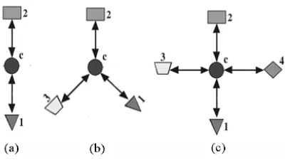
[image:15.612.214.414.233.349.2]

2.2

Star-Structured Heterogeneous Data Co-Clustering

Figure 2.1: The Star-Structured High-order Heterogeneous Data.

In the case of a Star-Structured Heterogeneous Data, a central data object is connected to

other types to form a star structure of the interrelationships as shown in Figure 2.1. Gao et

al. [15] proposed Consistent Bipartite Graph Co-clustering (CBGC) for clustering this kind

of data. Long et al. [24] proposed a spectral-clustering-based approach for multi-type

rela-tional data that generalized the approach for higher-order heterogeneous data co-clustering.

In [31] [25], Rege et al. proposed the Consistent Isoperimetric High-order Co-clustering

(CIHC) framework for partitioning the star-structured graphs. The proposed algorithm

partitions fusion of bipartite graphs. The algorithm is quick since it obtains a solution to

a sparse system by solving linear equation simultaneously. Long et al. [23] formulated

heterogeneous co-clustering as collective factorization on related matrices and obtained

co-clustering by deriving sub-matrices by simultaneously clustering multi-type interrelated

data. This algorithm provides more flexibility toward heterogeneous co-clustering since

the framework is applicable for general case data interrelationship.

(16)

being positive. This can be difficult to interpret for applications like documents and

im-age clustering since they always have positive input. Matrix-factorization-based clustering

approaches have received increased attention due to their applicability to high dimensional

datasets. Chen et al. [7] proposed non-negative matrix factorization for heterogeneous data

co-clustering. They performed trifactorization using an iterative algorithm to obtain new

cluster indicator matrices and the correlation between interrelated data. They show that

non-negative factorization outperforms graph-based methods and is less memory intensive.

Hence, they are efficient and scalable for large data.

2.3

Low-rank Matrix Approximation

Low-rank approximation methods extract correlation and then remove redundancy from

data to obtain sparse data [1]. One way to make clustering algorithms computationally

efficient is to integrate a data mining algorithm with low-rank approximation methods.

Singular Value Decomposition (SVD) is widely used for low-rank approximation since it

optimally calculates approximation using the Frobenius norm. However, SVD does not

produce a sparse matrix that is computationally very effective. Berry et al. [3] proposed an

improved low-rank approximation approach (Algorithm 844) called

quasi-Gram-Schmidt-algorithm based on the classical Gram-Schmidt quasi-Gram-Schmidt-algorithm. They trifactorized the input

matrix into two full-rank matrices and a non-singular matrix that is more efficient in terms

of computational power and space storage than SVD. Petros et al. [14] aims to address the

problem of memory access time (seek-time) for a large data set using the family of CUR

algorithms, namely LINEARTIMECUR and CONSTANTTIMECUR, based on fast Monte

Carlo algorithms. The LINEARTIMECUR algorithm makes use of the original data matrix

with two passes over existing storage of the matrix in external memory without storing on

RAM. The other algorithm, CONSTANTTIMECUR, focuses on optimization of seek time.

The advantage of the CONSTANTTIMECUR algorithm approach over the

(17)

however, it requires additional pass-over main memory, and the new low-rank

approxima-tion matrix has an addiapproxima-tional error. SVD and CUR are capable of identifying the correlaapproxima-tion

and hidden structure in a data set, but they are not efficient enough to obtain

computation-ally efficient sparse matrix. Sun et al. [34] addressed this problem by proposing a new

approximation method, the Compact Matrix Decomposition (CMD), which focuses on

re-ducing the high memory usage and computational cost for large sparse graphs. The authors

express the association between two nodes of graph using the relational matrix such that

every element represents the degree of similarity between two nodes of the object. They

removed the redundancy of nodes by sampling and removing the null row or column

en-tries and projecting original data into new subspace. Pan et al. [27] proposed a framework

(CRD) that achieves a linear-time low-rank approximation by utilizing sampling-based

ma-trix decomposition methods and perform partition-based co-clustering on large data. The

proposed framework decomposed the original data matrix into subsets of rows and columns

and performs co-clustering using matrix decomposition using an approach like block-value

decomposition [24]. Since subspace is created using random sampling, re-sampling is

needed to avoid a case where the entire cluster is not sampled while random sampling.

Chebyshevs Inequality was used to detect such rows and columns and reduce the error rate

because of biased sampling. Low-rank algorithms like CUR and CMD focused on

preserv-ing sparsity in large-graph data by creatpreserv-ing a smaller subspace to represent original data

by sampling it. However, they were overly complicated and were not able to optimize the

sub-space calculation either with time or space. To address these issues, Tong et al. [36]

proposed two algorithms, Colibri-S and Colibri-D, for static and dynamic graphs,

respec-tively. They proposed solution in which they first performed bias sampling by creating an

initial subspace that consisted of linearly dependent columns or near duplicates. Then they

optimized subspace by iterative sampling and removing all dependent columns or

dupli-cates. The authors showed that proposed algorithms for static and dynamic graphs are very

(18)

3. Evolutionary Star-Structured

Het-erogeneous Data Co-Clustering

In this chapter, I present an evolutionary star-structured heterogeneous data co-clustering

algorithm. Specifically, I will discuss 1) how to incorporate historical data into current

data and 2) how to efficiently infer clusters of different data types simultaneously using

non-negative matrix factorization (NMF).

3.1

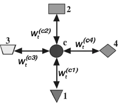
Evolutionary Star-Structured Heterogeneous Data

In the case of a Star-Structured Heterogeneous Data at a time stept, we represent multi-type

relational data of m-types using relational matrices with central data typecconnected top

other data types. The relation between every data type with central data type is represented

using relational matrix W(_tci)∈<nc×ni_{. For example in Figure 3.1, central data}_c_{is connected}

to four other data types, and we represent their relationship with central data type using

relational matrices W(_tc1), W(_tc2), W(_tc3), and W(_tc4), respectively.

3.2

Data dynamics and Low-rank Matrix Approximation

One of the challenges of evolutionary data is the dynamic nature of the data. Over a period

of time, we have changes in data size (changes in number of samples and features of data)

as well as changes in the structure of data (changes in number of clusters in the data).

Low-rank approximation methods extract correlation and then remove redundancy from data to

(19)

[image:19.612.214.411.91.266.2]

Figure 3.1: The Star-Structured Heterogeneous Data.

The family of Colibri methods [36], i.e., Colibri-S (Low-rank approximation method

for static data) and Colibri-D (Low-rank approximation for dynamic data), has proven more

efficient in terms of space and time compared to others like CRD [27], CMD [34], and CUR

[14]. Specifically, for dynamic data there is a gradual change in data between two

consec-utive time steps. Colibri-D takes leverage of the similarity between two consecconsec-utive time

steps to quickly update the approximating subspace. To integrate historic data into current

data, we make use of Colibri-D to obtain approximating historic subspace compatible with

respect to current data. First, we use the Colibri-S algorithm to calculate initial biased

sub-space [36]. Colibri-S iteratively constructs optimized subsub-space by eliminating redundant

columns. In the first stage, we simply follow the CUR [14] algorithm to sample a small

subset of columns from the data matrix with replacement, biased toward those with higher

norms. Then we initialize the output matrix with the first column of the data matrix and

then iteratively select a new column from biased subspace, which is linearly dependent on

the current columns. We finally obtain a matrix by removing all the redundant columns.

Colibri-D makes use of subspace calculated at timetto calculate subspace at timet-1. Since

the change in graph between two consecutive time steps is assumed to be reasonably small,

the overall edges affected between two time steps are far too less. Hence, for dynamic data,

(20)

a over period of time. So, authors have proposed a faster method to update output matrix

by sampling and comparing sampled edges between two time steps t andt-1. The output

thus obtained is compatible with respect to current data and is computationally efficient.

Before we apply low-rank approximation using the Colibri family to obtain sparse

com-patible historical data with respect to current data, we make sure the dimension of historical

data is larger than current data, so that when we apply Colibri-D, we get data dimensions

of historical data equal to that of current data. In the case where historical data has less

number of instances and/or features, we determine differences in instances and/or features

between historical data and current data, and we add those instances and/or features into the

historical data matrix. The inserted instance or feature receives the average of the whole

matrix at the current time step for each cell. We then apply Low-rank approximation to

project original dataW(_tci)∈<nc×ni _{into subspace}

f

Wt(ci)∈<nc×ni to improve computational efficiency of the algorithm in both time and space: clustering accuracy remains unaffected.

We define the overall cost function of EHCC (Evolutionary star-structured

Heteroge-neous Co-Clustering) as the sum of snapshot quality and historical cost. We solve this

problem by maximizing the clustering quality of the current snapshot and minimizing

the historical cost that provides clustering smoothness [6] [8] [38]. We propose an

op-timization equation to obtain EHCC for evolutionary higher-order relational data matrix

f

Wt

(ci)

∈<nc×ni _and_t_{= (}_t_,_t-1_{) as,}

J =min

L(₍c_t₎),M₍(_tci₎),R(₍i_t)₎≥0[α· kWft (ci)

−L(_tc)M_t(ci)R_t(i)k2

+(1−α)· kW]t−1 (ci)

−L(₍c_t₋)₁₎M₍(_tci₋)₁₎R(₍i_t)₋₁₎ k2_] _(3.1)

whereαis a trade off between historic data (historic quality) and current data (snapshot quality), and 0 ≤ α ≤ 1. L(_tc)∈<nc×kc _{(row coefficient matrix) and} _R(i)

t ∈<ki×ni (column

coefficient matrix) are indicator matrices representing soft-clustering for instances and

(21)

that represents the co-clustering relation between central data type and each data type

con-nected with central data type at time stept[24] [40] [7].

We generalize the optimization equation (3.1) for multiple time step data represented

by,Wf_t(ci)∈<nc×ni fort={1, 2,..., S}, where isSlast time-step in data,

J =min_L(c) (t),M

(ci) (t) ,R

(i) (t)≥0

PS

t=1α(1−α)

S−t_{· k}

f

Wt

(ci)

−L(_tc)M_t(ci)R(_ti)k2 _(3.2)

3.3

Estimating the Number of Clusters

In unsupervised learning methods, automatic estimation of number of clusters in data is

a challenging task [20]. For evolutionary data, the shape of data changes over a period

of time. We have change in the number of clusters over a period of time. For automatic

cluster estimation, we use six different well-known methods for cluster estimation, namely,

Silhouettes [32], Davies-Bouldin index [9], Calinski-Harabasz index [5], Krzanowski-Lai

index [21], and Hartigan [17] and weighted inter-to intra-cluster ratio with Homogeneity

and Separation index [35]. Because that data is gradually evolving, we make use of cluster

estimation on historical data to estimate the number of clusters in current data. The process

is faster since we need to estimate the number of clusters closer to the previously estimated

value only. We estimate the number of clusters using previously mentioned methods and

use the mode from the above estimation methods to decide the number of clusters in current

data.

3.4

Co-clustering using Non-negative Matrix Factorization

Since non-negative matrix-factorization-based co-clustering methods have been more

ef-ficient than graph-based methods in terms of efficiency and accuracy for large data sets

like document and image clustering, and they are easy to interpret, we use a non-negative

factorization-based method to obtain co-clustering. The minimization of (3.2) can be

(22)

optimization problem (3.2) through following the iterative solution to obtainL(_Sc), R(_Si) and

M(_Sci)[38]. This iterative process seeks to the minimize equation as rules specified in

(23)

Algorithm 1Evolutionary Star-Structured Heterogeneous Data Co-Clustering

Input: A relational matrixWt(ci)∈<nc×ni fort={1, 2,..., S}

Output: L(_tc)∈<nc×kc _{(row cluster indicator matrix) and} _R(i)

t ∈<ki×ni (column cluster

indicator matrix) andM(_tci)∈<kc×ki _{(block value matrix)}

1: fort←2, Sdo

2: fori←1, pdo{//If time-step Wt−1has less number of instances than Wt, add new instances to Wt−1 }

3: iflengthof(W_t(₋ci₁))< lengthof(W_t(ci))then 4: forj ←lengthof(W_t(₋ci₁)), lengthof(W_t(ci))do 5: insert⇐µ(Wt)

6: add instanceinserttoW_t(₋ci₁)

7: end for

8: end if

{//If time-step Wt−1 has more number of instances than Wt, add new instances to

Wt−1 }

9: iflengthof(W_t(₋ci₁))> lengthof(W_t(ci))then

10: Use intermediate results from the Colibri method to get unique and

inde-pendent subspace fromW_t(₋ci₁) equivalent to length ofW_t(ci) 11: end if

{//If time-step Wt−1has fewer features than Wt, add new instances to Wt−1}

12: iff eaturelengthof(W_t(₋ci₁))< f eaturelengthof(W_t(ci))then 13: forj ←f eaturelengthof(W_t(₋ci₁)), f eaturelengthof(W_t(ci))do 14: insert⇐µ(W_t(ci))

15: add featureinserttoW_t(₋ci₁)

16: end for

(24)

18: if f eaturelengthof(W_t(₋ci₁)) > f eaturelengthof(W_t(ci)) then {//If time-step Wt−1 has more features than Wt, add new instances to Wt−1}

19: Use intermediate results from the Colibri method to get unique and

inde-pendent subspace fromW_t(₋ci₁) equivalent to feature length ofW_t(ci) 20: end if

{//Use the Colibri-D method to obtain Low-rank approximation of Wt−1 with

respect toWt}

21: T EM P W_t(₋ci₁) ⇐Colibri−D(W_t(₋ci₁), W_t(ci)) 22: Wft

(ci)

⇐α·W_t(ci)+ (1−α)·T EM P W_t(−ci1))

23: end for 24: end for

25: Estimate number of cluster inWf_t

(ci)

using methods mentioned in section 3.3.

26: Obtain clustering using the following rules by applying recursive onWft

(ci)

L(₍c_S)₎₍_ab₎←L(₍c_S)₎₍_ab₎

Pp

i=1((

PS

t=1α(1−α)

S−t_·_W](ci) t )R

(i) (S)

T

M₍(_Sci₎)T)ab

Pp

i=1(L (c) (S)M

(ci) (S)R

(i) (S)R

(i) (S)

T

M₍(_Sci₎)T)ab

(3.3)

R₍(_Si)₎₍_ab₎←R(₍i_S)₎₍_ab₎(M

(ci) (S)

T

L(₍c_S)₎T(PS

t=1α(1−α)

S−t_·_W](ci)

t ))ab

(M₍(_Sci₎)TL₍(_Sc)₎TL(₍c_S)₎M₍(_Sci₎)R(₍i_S)₎)ab

(3.4)

M₍(_Sci₎₍)_ab₎ ←M₍(_Sci₎₍)_ab₎(L

(c) (S)

T

(PS

t=1α(1−α)S

−t_·_W](ci) t )R

(i) (S)

T

)ab

(L(₍c_S)₎TL(₍c_S)₎M₍(_Sci₎)R(₍i_S)₎R(₍i_S)₎T)ab

(3.5)

subject to the constraints∀ab: L

(c)

S ab≥0 and R

(i)

S ab≥0, wherek.kdenote Frobenius matrix norm, L(_Sc)∈<n×k_{, M}(ci)

S ∈<

k×l _{, R}(i)

S ∈<

(25)

4. Experiments

In this chapter, we demonstrate the performance of EHCC. We evaluated proposed

algo-rithm on variety of datasets, synthetic as well as real world datasets. Section 4.1 describes

datasets and preprocessing information. In section 4.2, we describe experiment evaluation

method. Finally, in section 4.3, we explain experiment and results.

4.1

Data Description and Preprocessing

We performed two sets of experiments to determine validity of proposed algorithm. We

run first set of experiments on a synthetic dataset, generated to evaluate different proposed

functionalities of the algorithm. For the second set, we used real world datasets from

three different domains, viz. web-service data, publicly available text-datasets, and image

dataset.

4.1.1

Synthetic Data

We performed two different experiments on synthetic data to test different features of

pro-posed algorithm. The first experiment demonstrates the ability of the algorithm to

han-dle instance and/or feature evolution, addition of instances and/or features, removal of

instances and/or features as well as the consistency across similar time-steps. The

sec-ond experiment shows algorithm’s ability to handle cluster shift over period of time. The

experiment tests instance as well as feature drift.

We generated a synthetic dataset consisting 8 time-steps, with step having 5 clusters of

200 instances. For initial time-step, the 5 clusters were generated from 5 normal

(26)

each cluster Cn, the distribution is determined by equation,µn=µn−1+ 5·n+R, where R is an integer randomly selected from [0-100]. For all distribution, standard deviation, σ

is equal to 1.

4.1.2

Web-Service Community Formation

A WSDL document consists of five key components: types, messages, portType, binding,

and service. Inspired by information retrieval techniques [26], we model services and

op-erations as vectors of functional terms as these terms represent the functionalities that the

services or operations provide. We apply traditional data processing techniques, which

in-volve extraction, tokenization, stopword removal and stemming, to obtain the functional

terms from the five WSDL components. Extraction identifies the key terms in a WSDL

document. Since terms in WSDL documents are usually stored in composite format (e.g.,

groceryStoreFood), tokenization is used to derive simple terms (e.g., grocery, store, food).

Non-functional terms and WSDL specific keywords such as http, url, host are removed by

the means of stopword removal. Finally, stemming is applied to reduce different forms of

a term into a common root (e.g. write, writing, andwroteget reduced towrite). After data

processing is completed, each service and operation will be represented as a vector of their

respective functional terms. Using these vectors, we construct a term-by-service matrix

and an operation-by-termmatrix. The dataset represents a tri-type data environment with

terms as the central data type. Theterms-operations matrix consists of 384 terms and 72

operations. In the term-by-service matrix we have 384 terms and 97 services. Terms are

collected by processing WSDL files from 5 different domains, namely, Communication,

Education, Food, Medical and Travel. So, every data type has 5 clusters.

4.1.3

Text Co-clustering

In this section, we evaluate our proposed algorithm for word-document co-clustering by

(27)

Data Set No. of Docu-ments

No. of

Cate-gories

No. of Docu-ment clusters

England-Heart,re0 913 2 4

Graft-Phos,re0 831 2 4

ArachidonicAcids-Hematocrit,re0 812 2 4

[image:27.612.95.524.104.192.2]

Enzyme-Infections,re0 849 2 4

Table 4.1: Data sets for (word-document-category) co-clustering

OHSUMED collection [18]. Data setre0is subset of the Reuters-21578 text categorization

dataset [22]. We mix these datasets as below.

• Dataset England-Heart was created by mixing classes England and

Heart-Valve-Prosthesisfromoh0dataset.

• Classes Graft-Survival andPhospholipidsfrom oh5were mixed to form the

Graft-Phosdataset.

• ArachidonicAcids-Hematocrit was derived fromoh10using Arachidonic Acids and

Hematocritclasses.

• Enzyme ActivationandStaphylococcal Infectionswere mixed to obtain the

Enzyme-Infectionsdataset.

To analyze performance of the algorithm, we compared our results with [7] [13] [24].

We performed feature selection to select top 1,000 words. We construct document-category

matrix by calculating the probability of each document belonging to each category. For

each document, if any of the top 1,000 word occurs, then we considered word occurrence

1 else 0. Then, we calculated probability of one document belonging to a category as the

ratio of the sum of occurrence of selected top 1,000 words in this document to 1,000. We

mix dataset from OHSUMED collection withre0to form higher-order dataset. Tables 4.1

(28)

4.1.4

Image Co-clustering

For our experiments on image datasets, we chose images from Corel-CDs which contains

general-purpose images from different domains such as automobiles, landscape, animal,

automobiles, etc. For image co-clustering, we represented each image in the form of vector

of 45 color features, 42 texture features [43] [37]. 45 color features consist of color

chan-nels(RGB, 9 features, including mean, variance, and skewness of R, G, and B channels),

color coherence vector(CCV, 24 features), and color histogram (CH, 12 features). Gabor

wavelet based texture (Gab, 24 features), edge direction histogram (EDH, 9 features), and

edge direction coherence vector (EDCV, 9 features) were extracted from each image to

represent image using Texture features. We constructed two matrices, image-color and

image-texturerepresenting color and textures features respectively.

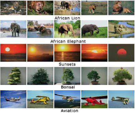
We selected 500 images from 5 different contents, namely,African Lion, African

Ele-phant, sunsets, bonsai, and aviation. Some examples from each category are shown in

Figure 4.1. In the proposed relevance feedback framework, we collect the users’ positive

feedback as samples to construct image-log matrix. Through feedback, the images marked

indicate that they are similar to each other according to user’s preference also called as a

log. In every log, user marks 3-5 similar images from 20 images randomly selected from

image pool. We mark similar images by 1 for rest images inlog-imagesvector we mark 0

(29)

[image:29.612.94.526.88.453.2]

Figure 4.1: Image samples selected random from each image category

4.2

Evaluation Method

We calculate clustering accuracy using micro-averaged precision value, given by,

AC =

Pn

i=1Φ(Xi, Yi)

n (4.1)

where n is number of instances in central data type, Φ(Xi, Yi) is equal to 1 if assigned label Yi and true label Xi for instanceiis same, else it is 0. Since the algorithm is solved

(30)

experiment 20 times and chose to average them [7] [24].

We evaluated performance of evolutionary algorithm by comparing its performance

against individual clustering at a time-steptwithout considering historic data.

4.3

Experiment Results

4.3.1

Synthetic Data

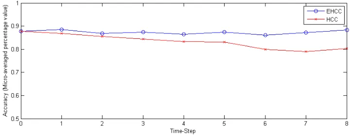
At time-step t1, Gaussian noise of 50 instances was added per cluster. At time-step t2

10 more instances were added from distribution of C2. At time-step t3 10 instances were

removed from cluster C4. At time-step t5, 2 features were added to C4. 1 feature was

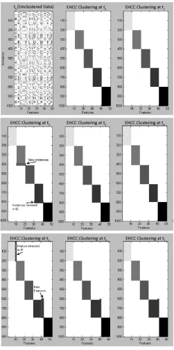
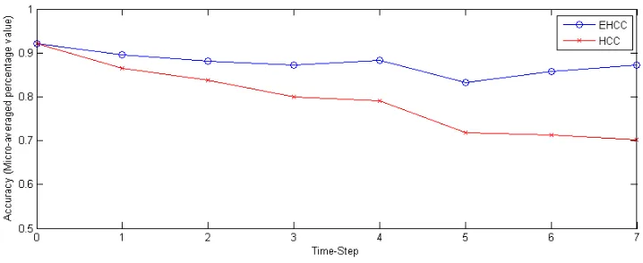
removed from C1 at time-step t6. t7 is unchanged from t6. Figure 4.2 shows visualization

of data over period of time from t0 to t7. In Figure 4.3, we show evolutionary higher order

clustering out performs higher order clustering. As proposed, the algorithm is capable of

handling data dynamics over period of time. At time-step t1, despite of adding Gaussian

noise, clustering at t1, is almost unchanged. At time-steps t2additional instances from same

distribution of clusters were added to dataset, and algorithm is capable of appropriately

clustering them. Similarly, at t3, we removed 10 instances from a cluster, and algorithm

produced stable results opposing the process of removal of instance over period of time.

At t4, data as well clustering remained unchanged, indicating stability of the algorithm

when data is unchanged. At time-step t5, the algorithm has clustered added features C4.

Even though the accuracy of algorithm slightly decreased, however, it has performed well

than static higher order co-clustering. Similarly, when we removed feature from dataset,

algorithm has shown resistance to the change in clustering at time-step t6. Clustering at t7

(31)

[image:31.612.184.435.88.592.2]

Figure 4.2: Visualization of Synthetic data clustering over period of time from t0to t7 : At

time-step t1, Gaussian noise of 50 instances was added per cluster. At time-step t210 more

instances were added from distribution of C2. At time-step t3 10 instances were removed

from cluster C4. At time-step t5, 2 features were added to C4. 1 feature was removed from

(32)

[image:32.612.129.488.96.243.2]

Figure 4.3: Comparison between accuracy of Evolutionary Higher order clustering(EHCC)

and Higher order Clustering(HCC) for Synthetic dataset

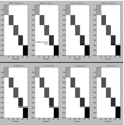
To evaluate algorithm’s ability to handle instance drift, we augmented original dataset.

We chose and modified of 20 instances from cluster C4. At each time-step, we progressively

modified the distribution of those instances towards C5so that at time step t7those instances

originally from C4 have same distribution as those in C5. In other words, we progressively

moved them from C4 to C5 over period of time. From Figure 4.4 shows clustering of data

over period of time. We show instances are progressively drifted from C4to C5over period

(33)

[image:33.612.94.528.87.523.2]

Figure 4.4: Visualization of Synthetic data clustering over period of time from t0to t7:t0is

the original data. Between time steps t1 - t6, instances shown drift from C4 to C5. Finally,

at time step t7, 20 instances moved from C4 to C5.

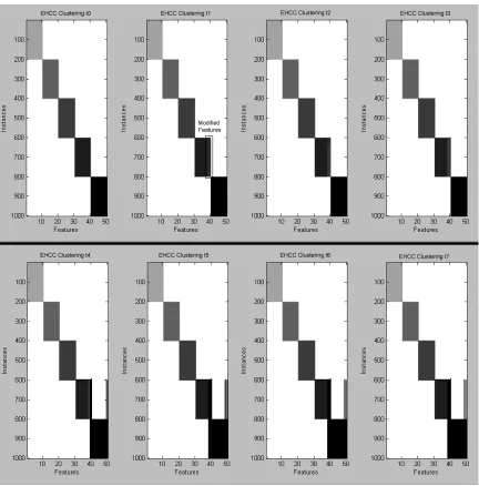
To evaluate algorithm’s ability to handle feature drift, we augmented original dataset.

We chose and modified of 2 features from cluster C4. At each time-step, we progressively

modified the distribution of those features towards new cluster C6 so that at time step t7

(34)

words, we progressively moved them from C4 to C6 over period of time. A new cluster

started appearing at t4. At t5both features moved to same cluster to form C6. Over next few

[image:34.612.94.526.159.597.2]

time steps, cluster has become more homogeneous. Figure 4.5 illustrate our observations.

Figure 4.5: Visualization of Synthetic data clustering over period of time from t0 to t7 :t0

is the original data. Between time steps t1- t6, features shown drift from C4 to new cluster

C6. At time step t5, 2 features moved from C4to C6. Over next few time steps, C6 became

(35)

4.3.2

Web-Service Community Formation

We augmented dataset into evolutionary one, by modifying instances and features. We

ob-tained distribution for each cluster and fort1andt2, we modified 5% instances and features

from each cluster using by randomly generating instances and features from distribution of

clusters they belong to. For t3 and t4, we modified 5% instances and features from each

cluster using by randomly generating instances and features from distribution of different

cluster. Att5, we added 5% new instances to cluster C3 generated from distribution of C3.

Similarly, At t6, we added 5% new features to C1 generated from distribution of C1. For

t7, we added 5% instances and features to instance and feature cluster C2 from instance

cluster C4 and feature cluster C5 respectively. At time-step t8, we removed 1% instances

[image:35.612.135.489.348.489.2]

and features each instance and feature cluster.

and Higher order Clustering(HCC) for Web-service dataset

Similar to synthetic data, for web-service data algorithm shows ability to handle data

dynamics. Figure 4.6 underlines algorithm’s ability to resists data changes. At time-stept7,

where we added instances as well as features to the data, static algorithm fail to perform,

where as proposed algorithm has excellently handled data changes. Similarly for time-step

t₈, when we removed instances and features from all clusters, our algorithm outperformed

(36)

4.3.3

Text Co-clustering

We augmented dataset into evolutionary one in similar way as we did for the web-service

[image:36.612.134.488.175.317.2]

dataset in section 4.3.2.

and Higher order Clustering(HCC) for Text dataset,England-Heart,re0

[image:36.612.128.488.408.550.2]

(37)

[image:37.612.129.487.94.237.2]

and Higher order Clustering(HCC) for Text dataset,ArachidonicAcids-Hematocrit,re0

Figure 4.10: Comparison between accuracy of Evolutionary Higher order

cluster-ing(EHCC) and Higher order Clustering(HCC) for Text dataset,Enzyme-Infections,re0

Through these experiments, we tried to test algorithm for text-datasets. Figures 4.7,

4.8, 4.9, and 4.10 further outline algorithm’s abilities to handle evolutionary data.

4.3.4

Image Co-clustering

For first experiment on image dataset, we increase the number of logs per category over the

period of timet0 tot10. We mark all clusters distinctly with logs, so over period of time,

[image:37.612.134.488.330.471.2]

(38)

identified. Then, we compare results for evolutionary algorithm with two different values

[image:38.612.110.491.180.478.2]

of trade off factorα, which equal to 0.8 and 0.2. This experiment also highlights algorithms ability of historic knowledge.

Figure 4.11: Comparison between evolutionary higher order clustering algorithm (EHCC) and Static Higher order clustering algorithm (HCC), and comparison of performances of evolutionary algorithm with respect to trade-of factorα

In Figure 4.11, we compare evolutionary with static version of higher order co-clustering.

As expected, evolutionary algorithm produces more accurate results than static version of

higher-order co-clustering algorithm. In stead, over period of time, evolutionary algorithm

produces more accurate results because of its capability of integration of historic

(39)

For second experiment, initially, we markedAfrican LionandAfrican Elephantbelong

to same clusters. Over the period of time t₀ to t₇, we marked them separately into two

clusters. We want to show, our proposed algorithm is able to handle cluster evolution over

period of time. Again, we performed experiment for two different values of trade-off values

[image:39.612.126.488.223.524.2]

to understand significance of integration of historic data.

Figure 4.12: Change in number of clusters over period of time, for evolutionary higher order clustering algorithm (EHCC) and Static Higher order clustering algorithm (HCC); and comparison of performances of evolutionary algorithm with respect to trade-of factor

α

From Figure 4.12, we show that, algorithm resists change in data. Our algorithm

indi-cates new cluster, i.e. 5th _{cluster, is formed at time-step} _t

2, even though we have started

marking 5th from time-stept1. So, new cluster is not formed till we have enough number

(40)

gave more importance for historical data, cluster change occurred more gradually. Hence,

[image:40.612.113.492.162.455.2]

the fifth image cluster was detected one time-step later att₃.

Figure 4.13: Number of instances in 5thcluster over period of time, for evolutionary higher order clustering algorithm (EHCC) and Static Higher order clustering algorithm (HCC); and comparison of performances of evolutionary algorithm with respect to trade-of factor

α

In Figure 4.13, we show number of instances clustered into 5th_{. We can observe period}

time 5th cluster has become more prominent over period of time. As shown earlier, when

(41)

5. Conclusion

I have proposed an evolutionary star-structured heterogeneous data co-clustering algorithm.

The research addresses unexplored avenues in clustering evolving star-structured

hetero-geneous data. The algorithm augment the current data with the historical data using cost

functions. Then it perform non-negative matrix factorization on the augmented current data

to obtain clustering. To evaluate the proposed work, I have applied our approach to diverse

domains: web-service community discovery, text mining and image clustering. Synthetic

and real world and publicly available text and image datasets validate the proposed

method-ology.

Further experimentation will be necessary to determine possible applications based on

my current research. An interesting direction would be tracking and analysis in social

gam-ing applications, blogs or a mashup of RSS feeds with daily updates, users, and words to be

clustered. Data dynamics has key effect on quality of the augmented matrix. So, additional

efforts are required to improve ability to handle data dynamics. In the proposed approach, I

have focused on a specific case of evolutionary heterogenous clustering. Further research is

necessary to improve ability of the algorithm to handle general case of heterogenous data.

The research will provide foundation for research on evolutionary heterogeneous data

clus-tering, hence opening many avenues for evolutionary clustering applications. This research

provides a road map for those that would venture to take on the endeavor of creating a novel

(42)

6. Acknowledgments

A grand thank you to Professor Rege, my committee, and Computer Science Department

and Rochester Institute of Technology for their assistance with this thesis. I would like to

take this opportunity to thank Hanghang Tong, Spiros Papadimitriou, Jimeng Sun, Philip

Yu, and Christos Faloutsos for making Colibri [36] implementation available for our

(43)

Bibliography

[1] Dimitris Achlioptas and Frank Mcsherry. Fast Computation of Low Rank Matrix Approximations. Journal of the ACM, 54(2):9–es, 2007.

[2] Arindam Banerjee, Inderjit Dhillon, Joydeep Ghosh, Srujana Merugu, and Dharmen-dra S Modha. A generalized maximum entropy approach to bregman co-clustering

and matrix approximation. Proceedings of the 2004 ACM SIGKDD international

conference on Knowledge discovery and data mining KDD 04, 8:509, 2004.

[3] Michael W. Berry, Shakhina A. Pulatova, and G. W. Stewart. Algorithm 844 :

Com-puting Sparse Reduced-Rank Approximations to Sparse Matrices. ACM Transactions

on Mathematical Software, 31(2):252–269, June 2005.

[4] Rui Cai, Lie Lu, and Alan Hanjalic. Unsupervised content discovery in composite

audio. Proceedings of the 13th annual ACM international conference on Multimedia

MULTIMEDIA 05, (december):628, 2005.

[5] T Calinski and J Harabasz. A dendrite method for cluster analysis. Communications

in Statistics Theory and Methods, 3(1):1–27, 1974.

[6] Deepayan Chakrabarti, Ravi Kumar, and Andrew Tomkins. Evolutionary clustering. In Proceedings of the 12th ACM SIGKDD international conference on Knowledge discovery and data mining - KDD ’06, page 554, New York, New York, USA, August

2006. ACM Press.

[7] Yanhua Chen Yanhua Chen, Lijun Wang Lijun Wang, and Ming Dong Ming Dong. Non-Negative Matrix Factorization for Semisupervised Heterogeneous Data Coclus-tering, 2010.

[8] Yun Chi, Xiaodan Song, Dengyong Zhou, Koji Hino, and Belle L Tseng. Evolutionary

spectral clustering by incorporating temporal smoothness. Proceedings of the 13th

ACM SIGKDD international conference on Knowledge discovery and data mining

(44)

[9] D L Davies and D W Bouldin. A cluster separation measure. IEEE Transactions on Pattern Analysis and Machine Intelligence, 1(2):224–227, 1979.

[10] Inderjit S Dhillon. Co-clustering documents and words using bipartite spectral graph

partitioning. Proceedings of the seventh ACM SIGKDD international conference on

Knowledge discovery and data mining KDD 01, pages(April 2006):269–274, 2001.

[11] Inderjit S Dhillon, Subramanyam Mallela, and Dharmendra S Modha. Information-theoretic co-clustering. Proceedings of the ninth ACM SIGKDD international confer-ence on Knowledge discovery and data mining KDD 03, 32(3):89, 2003.

[12] Chris Ding, Xiaofeng He, Richard F Meraz, and Stephen R Holbrook. A unified representation for multi-protein complex data for modeling protein interaction

net-works. PROTEINS: STRUCTURE, FUNCTION, AND BIOINFORMATICS, 57:99 –

108, 2004.

[13] Chris Ding, Tao Li, Wei Peng, and Haesun Park. Orthogonal nonnegative matrix

t-factorizations for clustering. Proceedings of the 12th ACM SIGKDD international

conference on Knowledge discovery and data mining KDD 06, 19(2):126, 2006.

[14] Petros Drineas, Ravi Kannan, and Michael W Mahoney. Fast Monte Carlo Algo-rithms for Matrices III: Computing a Compressed Approximate Matrix

Decomposi-tion. SIAM Journal on Computing, 36(1):184–206, 2006.

[15] Bin Gao, Tie-Yan Liu, Tao Qin, Xin Zheng, Qian-Sheng Cheng, and Wei-Ying Ma. Web image clustering by consistent utilization of visual features and surrounding

texts. In Proceedings of the 13th annual ACM international conference on

Multi-media, pages 112–121. ACM, ACM, 2005.

[16] Nathan Green, Manjeet Rege, Xumin Liu, and Reynold Bailey. Evolutionary spectral

co-clustering. The 2011 International Joint Conference on Neural Networks, pages

1074–1081, July 2011.

[17] J A Hartigan. Clustering Algorithms, volume 2 of Wiley Series in Probability and

Mathematical Statistics. John Wiley & Sons, 1975.

[18] William Hersh, Chris Buckley, T J Leone, and David Hickam. OHSUMED: An inter-active retrieval evaluation and new large test collection for research. In W Bruce Croft

(45)

SIGIR conference on Research and development in information retrieval, volume 17

ofSIGIR ’94, pages 192–201. Springer-Verlag New York, Inc., 1994.

[19] A K Jain, M N Murty, and P J Flynn. Data clustering: a review. ACM Computing

Surveys, 31(3):264–323, 1999.

[20] Anil K Jain. Data clustering: 50 years beyond K-means. Pattern Recognition Letters, 31(8):651–666, 2010.

[21] W J Krzanowski and Y T Lai. A Criterion for Determining the Number of Groups in a Data Set Using Sum-of-Squares Clustering. Biometrics, 44(1):23–34, 1988.

[22] David D Lewis, Yiming Yang, Tony G Rose, and Fan Li. RCV1: A New Benchmark Collection for Text Categorization Research. Corpus, 5:361–397, 2004.

[23] Bo Long, Zhongfei Mark Zhang, Xiaoyun W´u, and Philip S Yu. Spectral clustering for multi-type relational data. Proceedings of the 23rd international conference on Machine learning ICML 06, pp:585–592, 2006.

[24] Bo Long, Zhongfei Mark Zhang, and Philip S Yu. Co-clustering by block value

decomposition. Proceeding of the eleventh ACM SIGKDD international conference

on Knowledge discovery in data mining KDD 05, page 635, 2005.

[25] Manjeet Rege and Qi Yu. Efficient Mining of Heterogeneous Star-Structured Data.

International Journal Software and Informatics, 2(2):141–161, 2008.

[26] Christopher D Manning, Prabhakar Raghavan, and Hinrich Sch¨utze. Introduction to

Information Retrieval, volume 1. Cambridge University Press, 2008.

[27] Feng Pan, Xiang Zhang, and Wei Wang. A General Framework for Fast Co-clustering

on Large Datasets Using Matrix Decomposition.Proceedings / ACM-SIGMOD

Inter-national Conference on Management of Data. ACM-Sigmod InterInter-national Conference

on Management of Data, 24:1337–1339, April 2008.

[28] Ruggero G Pensa. Constrained Co-clustering of Gene Expression Data. Gene, pages

25–36, 2008.

[29] Manjeet Rege, Ming Dong, and Farshad Fotouhi. Co-clustering Documents and

Words Using Bipartite Isoperimetric Graph Partitioning. Sixth International

(46)

[30] Manjeet Rege, Ming Dong, and Farshad Fotouhi. Co-Clustering Image Features and

Semantic Concepts. In 2006 International Conference on Image Processing, pages

137–140. IEEE, 2006.

[31] Manjeet Rege, Ming Dong, and Jing Hua. Clustering web images with multi-modal

features. Proceedings of the 15th international conference on Multimedia -

MULTI-MEDIA ’07, page 317, 2007.

[32] P Rousseeuw. Silhouettes: A graphical aid to the interpretation and validation of

cluster analysis. Journal of Computational and Applied Mathematics, 20(1):53–65,

1987.

[33] Amit Salunke, Minh Nguyen, Xumin Liu, and Manjeet Rege. Web service

discov-ery using semi-supervised Block Value Decomposition. In2011 IEEE International

Conference on Information Reuse & Integration, pages 36–41. IEEE, August 2011.

[34] Jimeng Sun, Yinglian Xie, Hui Zhang, and Christos Faloutsos. Less is More: Sparse

Graph Mining with Compact Matrix Decomposition. Stat. Anal. Data Min., 1(1):6 –

22, 2008.

[35] Kadim Tas. A new cluster validity index for prototype based clustering algorithms based on inter- and intra-cluster density. Proc Int Joint Conf on Neural Networks, 2007(Ijcnn):12–17, 2007.

[36] Hanghang Tong, Spiros Papadimitriou, Jimeng Sun, Philip S Yu, and Christos Falout-sos. Colibri: fast mining of large static and dynamic graphs. Database, pages 686– 694, 2008.

[37] A Vailaya and A Jain. On image classification: city vs. landscape, 1998.

[38] Lijun Wang, Manjeet Rege, Ming Dong, and Yongsheng Ding. Low-Rank Kernel Matrix Factorization for Large Scale Evolutionary Clustering. IEEE Transactions on Knowledge and Data Engineering, 99(PrePrints):1–15, 2010.

[39] Guandong Xu, Yu Zong, Peter Dolog, and Yanchun Zhang. Co-clustering Analysis of

Weblogs Using Bipartite Spectral Projection Approach. KES, pages 398–407, 2010.

[40] Wei Xu, Xin Liu, and Yihong Gong. Document clustering based on non-negative

matrix factorization. Proceedings of the 26th annual international ACM SIGIR

(47)

[41] Sungroh Yoon, Luca Benini, and Giovanni De Micheli. Co-clustering: A Versatile Tool for Data Analysis in Biomedical Informatics. IEEE transactions on information technology in biomedicine a publication of the IEEE Engineering in Medicine and

Biology Society, 11(4):493–494, 2007.

[42] Qi Yu and Manjeet Rege. On Service Community Learning: A Co-clustering

Ap-proach. 2010 IEEE International Conference on Web Services, pages 283–290, 2010.

[43] Hongjiang Zhang, Hewlett-packard Laboratories, and Palo Alto. Benchmarking of

Image Features for Content-based Retrieval. Conference Record of Thirty-Second

Theses

Thesis/Dissertation Collections