Application of the factorisation method to limited aperture ultrasonic phased array data

(1)

Application of the Factorisation Method to

Limited Aperture Ultrasonic Phased Array Data

Katherine M. M. Tant1)_{, Anthony J. Mulholland}1)_{, Anthony Gachagan}2)

1)_{Department of Mathematics and Statistics, University of Strathclyde, Glasgow, UK. [email protected]} 2)_{Centre for Ultrasonic Engineering, University of Strathclyde, Glasgow, UK}

Summary

This paper puts forward a methodology for applying the frequency domain Factorisation Method to time domain experimental data arising from ultrasonic phased array inspections in a limited aperture setting. Application to both synthetic and experimental data is undertaken and a multi-frequency approach is explored to address the difficulty encountered in empirically choosing the optimum frequency at which to operate. Additionally, a trun-cated singular value decomposition (TSVD) approach is implemented in the case where the flaw is embedded in a highly scattering medium, to regularise the scattering matrix and minimise the contribution of microstructural noise to the final image. It is shown that when the Factorisation Method is applied to multi-frequency scatter-ing matrices, it can better characterise crack-like scatterers than in the case where the data arises from a sscatter-ingle frequency. Finally, a volumetric defect and a lack-of-fusion crack are both successfully reconstructed from ex-perimental data, where the resulting images exhibit only 3% and 10% errors respectively in their measurement.

© 2017 The Author(s). Published by S. Hirzel Verlag·EAA. This is an open access article under the terms of the Creative Commons Attribution (CC BY 4.0) license (https://creativecommons.org/licenses/by/4.0/).

PACS no. 43.35.-c, 43.35.Zc

1. Introduction

Ultrasonic nondestructive testing uses high frequency me-chanical waves to inspect components of safety criti-cal structures, ensuring that they operate reliably without compromising their integrity. It is routinely used within the non-destructive testing (NDT) industry due to the rel-atively inexpensive and portable equipment it requires and its potential for automation and real-time results. The pro-duction and implementation of ultrasonic phased array transducers (which are capable of simultaneously trans-mitting and receiving ultrasound signals across multiple array elements) has surged in the last ten years [1]. These multi-element transducers allow for greater coverage (and potentially faster inspection times) than that aﬀorded by single probe inspections, and provide the possibility of performing inspections with ultrasonic beams at various angles and focal lengths, giving rise to a richer set of data. When each of the N elements are ﬁred sequentially, the

N2_{time traces arising from each transmit-receive pair of} elements (N being the number of elements, usually be-tween 32 and 256) can be processed and stored in a 3D matrix (N ×N ×T, whereT is the number of sample points in the time domain), usually termed the Full Matrix Capture (FMC) [2].

Received 23 February 2017, accepted 7 August 2017.

The current industry benchmark for interpreting the FMC is the Total Focussing Method (TFM) [2]; a de-lay and sum imaging technique based in the time domain where the area of inspection is discretised into a grid and the signals from every transmit-receive pair are subse-quently focussed at each pixel and su mmed. In its most basic form, the TFM can struggle with the detection and characterisation of flaws embedded in highly heteroge-neous media. However, efforts have been made to improve the algorithm so that it can handle such environments. Modifications include the implementation of frequency fil-tering [3], the incorporation of the directional dependence of the ultrasonic velocity (caused by anisotropy) [4], and the consideration of multiple wave modes [5].

(2)

identiﬁ-cation. Other such methods include the Linear Sampling Method [16, 17], the Probe Method [17, 18] and the Sin-gular Sources Method [17, 19]. These sampling methods are so named since they work on the basis of determining whether sampled points within an imaging domain meet some criteria which determines whether they fall within the support of the ﬂaw domainD.

[image:2.595.270.504.59.155.2]

The NDT community have yet to fully explore the po-tential of the Factorisation Method for improved flaw char-acterisation and this paper endeavours to put forward a framework for applying it to time domain experimental data arising from limited aperture phased array inspec-tions. Some interesting work has already been carried out in [13, 20], where sampling methods were used to image cracks in acoustic waveguides, which of course has im-portant implications for the NDT of pipelines. However this work showed only results from simulated data with Gaussian noise and is limited to the inspection of plate-like structures. One important contribution of the work shown in this paper is that it presents a framework for interro-gating time domain ultrasonic phased array data arising from the inspection of welds, by the Factorisation Method. Application of sampling methods to time domain data has been studied before in [20, 21, 22, 23, 24] however the authors believe that this paper presents application of the Factorisation Method to experimentally collected time do-main ultrasonic phased array data in a limited aperture set-ting for the first time. The case where the host medium is inhomogeneous (resulting in poor signal to noise ra-tio) is first considered via synthetically generated data. The phased array inspection of a weld with a highly scat-tering material microstructure (taken from experimental electron backscatter diffraction (EBSD) measurements) is modelled within a finite element package. This allows us to study noisy signals which closer resemble the data aris-ing from experiment than those created when the simula-tion is run with a homogeneous host medium and then ret-rospectively perturbed by random noise. Note that the im-plementation of the factorisation methodology used in this paper assumes a homogeneous host medium and receives no information on the scattering host microstructure and so any inverse crimes are avoided. The reconstructions of both volumetric and crack-like scatterers embedded in this heterogeneous environment are presented. Crack-specific adaptations to the Factorisation method and the linear sam-pling method have been developed in [13, 25, 26, 27]. In the study by Boukari et al. [27], an expression for the far-field pattern of a smooth non intersecting open arc is presented and employed within the indicator func-tion used to reconstruct the scatterer. However, in [25], an open arc scatterer with Dirichlet boundary conditions is reconstructed using the far-field pattern for a point source. In this paper, on the grounds of simplicity, we will take the second approach. To begin, a brief overview of the method is given. The truncated singular value decompo-sition (TSVD) is used to regularise the scattering matrices that arise from the FMC data in the cases where the flaw is embedded in a highly scattering host medium. It is well known that the largest scatterers can be associated with the

Figure 1. Scattering problem geometry whereDis a volumetric scatterer with boundaryΓ,ui_{is the incident plane wave and}_us_is the resulting scattered ﬁeld.

largest eigenvalues of the scattering matrix [28] and so, by using the TSVD to set the smallest eigenvalues to zero, interference from microstructural heterogenetites (which can be thought of as noise) can be reduced, enhancing the signal to noise ratio of the resulting image.

Additionally, a multi-frequency approach, as previously explored in [29], is adopted. In taking a time windowed Fourier transform of collected time domain data, a range of scattering matrices spanning multiple frequencies is made available. Choosing the center frequency of the transducer does not necessarily give rise to the optimal reconstruction of the ﬂaw and an empirical strategy to choose the most appropriate frequency requiresa prioriknowledge of the defect’s characteristics. To avoid this, a multi-frequency approach is proposed, where the scattering matrices are summed over the range of frequencies which span the bandwidth of the transducer. As this approach allows in-creased exploitation of the available data, improved char-acterisation is subsequently facilitated.

2. The Factorisation Method

The forward scattering problem states that there is an in-cident plane wave, ui₍_{x, θ}₎ ₌ _eikx·θ_{, x} _∈ _R_{, travelling in}

directionθ ∈ S2_{, where}_S2 ₌_{_x _∈_R3 _: _|_x_| ₌ ₁_}_{is the} unit sphere inR3_{. On encountering a defect, in this case} the region Dwith boundary Γ, the wave scatters, giving rise to the scattered ﬁeld us _{(see Figure 1). The sum of}

the incident and scattered fields results in the total fieldu, which satisfies the Helmholtz equation

Δu+k2_u ₌ _{0 outside}_D, ₍₁₎ subject to u = 0 onΓ,

where k is the wavenumber. Although we are primarily interested in the elastodynamic case for the purposes of NDT, by considering only longitudinal waves (mode con-version does occur however the method we use to extract the scattering matrices is based on first times of arrival and so is dominated by the longitudinal waves – see Section 3) then it is sufficient to study the Helmholtz equation. The scattered fieldus_{satisfies the So mmerfeld radiation}

con-dition

∂us

(3)

uniformly in all directions ˆx = x/|x|, ensuring that the wave is radiating outwards and decays suﬃciently fast so that there are no sources at inﬁnity.

The scattered ﬁeldus_{also solves the exterior Dirichlet}

problem

Δv+k2_v ₌ _{0 outside}_D, ₍₃₎ subject to v = f onΓ,

wheref = −ui _and_v_{satisﬁes the So mmerfeld radiation}

condition given in (2).

The Factorisation Method [10, 11, 12] attempts to solve the inverse problem of determining the shape ofD from the scattered ﬁeld. The methodology exploits the relation-ship between the data-to-pattern operatorGand the shape of the scatterer. To begin with, letusph _{be the}

fundamen-tal, radiating solution to the Helmholtz equation inR3 _(a spherical wave generated at a point sourcezand measured at pointx, in a homogeneous host medium) given by

usph₍_{x, z}₎₌ eik|x−z|

4π|x−z|, x, z∈R3, x=z. (4) As the distance betweenxandzgets large (far-ﬁeld), the spherical wave begins to resemble a plane wave at pointx. This can be approximated by

u∞_{( ˆ}_x₎₌_e−ikxˆ·z_, _x_ˆ _∈_S2_, ₍₅₎ whereu∞_{is the far-ﬁeld pattern when we have an incident} wave arising from a point source.

The Herglotz wave function describes the superposition of plane waves

Hg(x) :=

S2

eikx·θ_g₍_θ_{) d}_{θ, x}_∈_Γ_, ₍₆₎

with densityg∈L2₍_S2_{). The far-ﬁeld pattern arising from} an incident plane wave applied to some functiong is the far-ﬁeld pattern of the Herglotz wave function with density

g. By denoting the far-ﬁeld pattern of the scattered ﬁeld (obtained from our measured data), byu∞

s, we can deﬁne

the far-ﬁeld operatorF by

F g( ˆx)=

S2u

∞

s( ˆx, θ)g(θ) ds(θ) for ˆx∈S2. (7)

Note thatF is a normal operator and compact inL2₍_S2_). Deriving the following factorisation of the operatorF [10, Theorem 1.15],

F =−GP∗_G∗_, ₍₈₎ is the basis for the Factorisation Method. Here P∗ _:

H−1/2₍_Γ₎_→_H1/2₍_Γ_{) is the}_L2_{adjoint of the single layer} boundary operatorP :H−1/2₍_Γ₎_→_H1/2₍_Γ₎

P ϕ(x)=

Γu

sph₍_{x, y}₎_ϕ₍_y_{) d}_s₍_y₎_{, x}_∈_Γ_. ₍₉₎

and eﬀectively converts the incoming wave to an outgoing wave on the defect boundary. The operatorG∗_:_L2₍_S2₎_→

H−1/2₍_Γ_{) is the}_L2_{adjoint of}_G_:_H1/2₍_Γ₎_→_L2₍_S2_{), the} data-to-pattern operator, deﬁned by

Gf=u∞_. ₍₁₀₎

Critically, the rangeR(G) of the operatorG has a direct relationship to the shape of the domain D. Forz ∈ R3_,

φz∈L2(S2) is deﬁned by

φz( ˆx)=e−ikxˆ·z, xˆ∈S2. (11)

It follows that ifz∈D, then, from equations (5) and (11),

φz = u∞ and so, from equation (10), φz ∈ R(G) when

z∈D.

The converse is also true according to Theorem 1.12 in [10]. To gain an exact characterisation of R(G) in terms of the known operatorF, we can relateG toF by equation (8). To proceed, some further technical assump-tions are required. It is assumed thatF, for the Dirichlet boundary conditions (Equation 1), is normal, the operator

I+ikF/8π2_{is unitary and}_k2_{is not a Dirichlet eigenvalue} of−ΔinD(these conditions are justiﬁed in [10]). It then holds that the range of (F∗_F₎1/4_{coincides with that of}_G_. Hence, the sampling pointz∈R3_{lies in}_D_{if and only if}

F∗_F1/4_g₌_φ

z (12)

for someg∈L2₍_S2_).

By Picard’s criterion, equation (12) is solvable if and only if the conditionφz∈ R((F∗F)1/4) is satisﬁed (this is

shown to hold by equations (5)–(10)). It then follows that,

z∈Dif and only if ∞

j=1

|(φz, ψj)L2₍_S2₎|2

|λj| <∞, (13)

where {λj, ψj} forms an eigensystem of the normal

op-eratorF such that the eigenvectors deﬁne a complete or-thonormal system inL2₍_S2_{) and the Fourier coe}_ﬃ_cients decay to zero faster than the eigenvalues. Using the spec-tral theory of a normal operator, [10, equation 1.74] it is observed

(F∗_F₎−1/4_φ

z=

∞

j=1

1

|λj|

(φz, ψj)ψj (14)

⇐⇒ ∞

j=1

1

|λj|

(φz, ψj)

2

<∞, (15)

and so equation (13) does indeed hold. From equations (12) and (14), the solutiongis given by

g= j

φz, ψj_L2₍_S2₎

|λj|

ψj, (16)

and the following result is obtained

z∈D ⇐⇒ φz∈ R((F∗F)1/4) (17)

⇐⇒ W(z)=

j

|(φz, ψj)L2₍_S2)|2

|λj|

−1

(4)

In practice, we use theN×N scattering matrix in place of our operatorF (whereN is the number of array ele-ments). AssumingF is normal (and thus diagonalizable), it holds that there existN linearly independent eigenvec-tors. Thus, when using this discrete, limited aperture, we truncate equation (17) to

w(z)=

_N

j=1

|(φz, ψj)L2₍_S2)|2

|λj|

−1

> ε, z∈D, (18)

whereε >0. By plottingw(z) for all sampling points,z, it is possible to recover the shape and size of the defect.

2.1. TheF# Operator

It was shown above that a sampling pointzlies within the domainDof the scatterer if and only if there exists a so-lution inL2₍_S2_{) to equation (12). However, this criterion} only holds if the far-ﬁeld operatorF is normal, which is not always the case when limited angles of inspection or heterogeneous host materials are present. To circumvent this, the positive, self-adjoint operator F# is introduced [10, 30] where

F#=|Re(F)|+|Im(F)|, (19)

and

Re(F)= 1₂(F+F∗_{) and} _Im₍_F₎₌ 1

2i(F−F∗). (20)

It is helpful to note here that for a given self-adjoint oper-atorJ, if

J = ₊_∞

−∞λdEλ, (21)

then

dJ:= ₊_∞

−∞

_λ_d_E_λ_, ₍₂₂₎

where Eλ is the spectral family of the operator J [13].

AsF is compact inL2₍_S2_{) it follows that}_F∗ _{is compact} inL2₍_S2_{) and thus so is}_F

# [31]. It can be subsequently shown that a sample pointz belongs to the domainDif and only if the integral equation

F_#1/2g =φz (23)

has a solution in L2₍_S2_{) [10] (here} _φ_z _{is as deﬁned in} equation (11)). It follows that, by plotting

W(z)=

_N

j=1

|(φz, ψj#)L2₍_S2₎|2

|λ#

j|

−1

, z∈R2_, ₍₂₄₎

where {λ#

j, ψj#}j∈N forms an eigensystem of the self-adjoint operator F# such that the eigenvectors deﬁne a complete orthonormal system inL2₍_S2_{), an image of the} scatterer can be reconstructed.

2.2. Truncated SVD of the Scattering Matrix

From equation (24), we can see thatW(z) is large when

φz is orthogonal to the eigenvectors ofF#, which occurs when the sampling point lies within the spatial domain oc-cupied by the ﬂaw. The other occasion whenW(z) could be large is whenλ#

j is large for somej = 1, . . . , N, even

whenz∈Dand so (φz, ψj#)L2₍_S2₎=0.

To minimise the contribution of these cases, an artiﬁcial nullspace is created. This is achieved by taking the singu-lar value decomposition (SVD) of theN ×N scattering matrix,F∗_{, and approximating it using the}_m_largest sin-gular values via

F∗₌ m

n=1

σnunvn, (25)

thus creating a nullspace with dimension N−m. In the case of subwavelength non-isotropic scatterers, the largest eigenvalue is associated with the spherically sy mmetric part of the scattering amplitude and there are three eigen-values associated with the directional part [32, 33]. Where the scatterer is larger than the wavelength, there exist many singular values associated with it. And so, in the work be-low we make the constraint thatm ≥ 4. Aside from this lower bound, we typically assume that the singular val-ues which are greater than 10% of the largest singular value correspond to scattering by the defect and those be-low this threshold correspond to noise and scattering by the microstructure [15, 34]. However, by studying the dis-tributions of the singular values it can be observed that this threshold may not always be optimal and may require some tuning subject to the system parameters.

3. Application to NDT

The results in this paper arise from application of the Fac-torisation Method to data collected (or modelled) in the time domain. To interrogate the data using the Factori-sation Method, we require a frequency domain represen-tation of the scattered signals over a time interval corre-sponding to the wave’s interaction with the flaw. To ensure that the flaw scattering dominates in the frequency domain and that other experimental artifacts (such as the back wall of the sample) don’t obscure the flaw’s scattering signa-ture, the time domain FMC data must be processed. Firstly the location of the flaw is requireda priori(it must be re-membered that the Factorisation Method is being applied here as a post-imaging tool for flaw characterisation). In this paper, the defect is located using an image generated by the standard TFM [2]

I(x, z)= (26)

N

s,r=1

As,r

(xs−x)2+z2+

(xr−x)2+z2

c

,

(5)

[image:5.595.24.507.57.543.2]

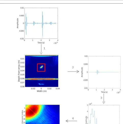
Figure 2. Processing of time domain FMC data for extraction of scattering matrices. Firstly the ﬂaw is located using the standard TFM. Then, the distance of the defect from the array coupled with the estimated wave speed gives rise to a time interval pertaining to scattering by the defect. The Fourier transform is applied to the FMC data in this interval. Then, the amplitude at a speciﬁed frequency is plotted for each transmit-receive pair to generate the scattering matrix.

series data) when a wave is emitted at locationxsand

re-ceived at locationxr andcis the estimated constant wave

speed throughout the host medium. When the distance of the defect from the array is known, it can be coupled with the estimated wave speedcto give rise to a time pertaining to scattering by the defect. Some interval is taken around this value and a discrete Fourier transform is applied. From the resulting spectral data a scattering matrix can be gen-erated at a chosen frequency by plotting the amplitude of the power spectrum at that frequency for every transmit-rece ive pair. The scattering matrix is then assigned as the operatorF and the Factorisation Method can be applied

accordingly. This process is depicted in Figure 2 and can be summarised in four key steps:

1. Apply the TFM algorithm (see equation (26)) to the raw FMC data to ﬁnd the location of the defect. 2. For each pair of transmit-receive elements, calculate the

distance from the transmitterxsto the centre of the

de-fect in the TFM image and back to the receiverxr.

Cou-pled with the wavespeed in the material,c, calculate the point of interest in time,ts,r. Take an interval centered

roundts,ron each set of time series dataAs,r.

(6)

4. The amplitude of Ys,r at a speciﬁc frequencyf is

as-signed as the elementFs,rof the scattering matrixF at

that frequency.

Note that the size of the time interval depends on the size of the defect and its proximity to other scatterers (we would ideally not incorporate data arising from other scat-terers within the interval). It is clear that, for every FMC dataset there exists a set of scattering matrices, each one at a different frequency. Choosing a frequency at which to operate is not straightforward: the best reconstructions rarely arise from the scattering matrix generated at the center frequency of the transducer. Identifying which sin-gle frequency results in the optimal reconstruction of the flaw requiresa prioriknowledge of the defect dimensions. Hence, a multi-frequency approach (where scattering ma-trices spanning at least the−6 dB bandwidth of the trans-ducer are summed at regular intervals) is introduced, ex-ploiting more of the information made available by the bandwidth of the transducer whilst removing the subjec-tive aspect of identifying the frequency which affords the best flaw reconstruction.

3.1. Simulated and Experimental Data Sets

[image:6.595.271.503.100.213.2]

In this paper, the Factorisation Method is applied to data arising from two sources. Firstly, the scattering of an ultra-sonic wave by a flaw is simulated using a time domain fi-nite element method in the software package PZFlex [35]. In this paper, three FMC datasets generated using this method are examined (the parameters are listed in Tables I and II). Firstly the scattering by a 5 mm crack with 40◦ orientation (relative to the horizontal axis) embedded in a homogeneous medium was simulated. The same flaw was then placed in a heterogeneous environment where the lo-cally anisotropic microstructure of an austenitic steel weld (derived from experimental electron backscatter diff rac-tion measurements [36]) was embedded in the simularac-tion (see Figure 3). In both instances the domain was meshed with elements of dimension λ/15, where lambda is the wavelength. The 1.5 MHz sinusoidal excitation used thus gave rise to elements approximately 200 µm square, which is sufficient to accurately model the wave propagation. In the heterogeneous case, the weld structure consisted of grains where contigious crystallites with similar orienta-tions were grouped together to form locally anisotropic regions. The correlation length [37] was estimated asλ/8 and the RMS longitudinal velocity through this heteroge-neous medium was estimated as 5758 m/s with a standard deviation of 146 m/s (calculated using the times corre-sponding to the backwall echo in the A-scans where trans-mission and reception took place on the same element). The location of the flaw and this estimated average wave speed were then used to isolate the time interval pertaining to the flaw and the relevant scattering matrices were thus obtained (see Section 3 and Figure 2). Note that by isolat-ing the time interval usisolat-ing the estimated longitudinal ve-locity, shear wave scattering (which should occur at a later time) is neglected, as is secondary scattering which occurs after the wave has reflected offthe back wall and interacts

Table I. Parameters used in the FE simulation of an ultrasonic phased array inspection of an embedded 5 mm crack. H.M.: Ho-mogeneous Medium, M.I.: Microstructure Included.

H.M. M. I.

Number of Array Elements 64 64

Pitch 2 mm 2 mm

Transducer Center Frequency 1.5 MHz 1.5 MHz

Depth of Flaw 50 mm 50 mm

Depth of Sample 78.4 mm 78.4 mm

Material Density 7874 kg/m3 _{7874 kg/m}3

Estimated wave speed 5900 m/s 5758 m/s

[image:6.595.269.505.318.528.2]

(from TFM)

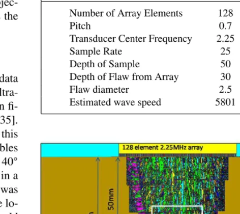
Table II. Parameters used in the FE simulation of an ultrasonic phased array inspection of an 2.5 mm diameter side-drilled hole.

Value Unit

Number of Array Elements 128

-Pitch 0.7 mm

Transducer Center Frequency 2.25 MHz

Sample Rate 25 MHz

Depth of Sample 50 mm

Depth of Flaw from Array 30 mm

Flaw diameter 2.5 mm

Estimated wave speed 5801 m/s

Figure 3. Geometry input to the ﬁnite element simulation where a 5 mm crack with 40◦_{orientation (relative to the horizontal axis)} is embedded in an austenitic weld microstructure. The 128 ele-ment 2.25 MHz array is placed directly above the ﬂaw over the weld material. The white box depicts the sampling domain.

(7)

[image:7.595.21.254.82.367.2]

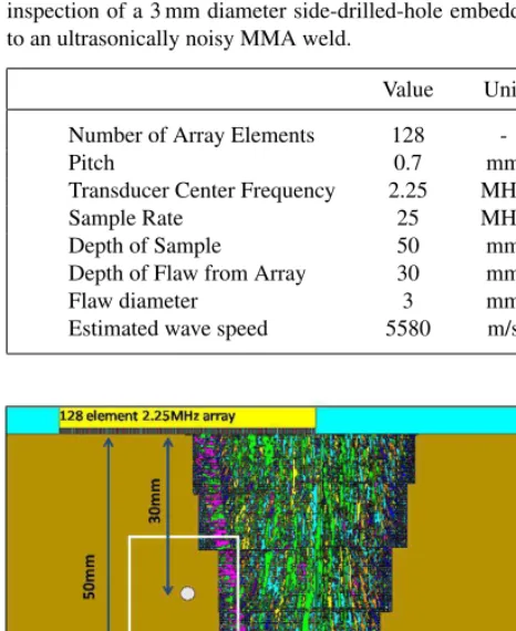
Table III. System parameters for the experimental phased array inspection of a 3 mm diameter side-drilled-hole embedded next to an ultrasonically noisy MMA weld.

Value Unit

-Pitch 0.7 mm

Transducer Center Frequency 2.25 MHz

Sample Rate 25 MHz

Flaw diameter 3 mm

[image:7.595.268.504.130.337.2]

Figure 4. Geometry input to the ﬁnite element simulation where a 2.5 mm diameter side-drilled hole is embedded in the parent ma-terial (stainless steel) close to a highly scattering polycrystalline region which represents an austenitic steel weld. The 128 ele-ment 2.25 MHz array is placed directly above the ﬂaw over the parent and weld materials. The white box depicts the sampling domain.

Secondly, the Factorisation Method was applied to ex-perimental data. The first test sample considered in this paper is a steel block containing an ultrasonically noisy manual metal arc (MMA) weld. The defect of interest is a 3 mm diameter side drilled hole lying to the left of the weld, 30 mm from the front face of the 50 mm thick sam-ple, as shown in Figure 5. The inspection was carried out by a 2.25 MHz linear array (Vermon, France) as specified in Table III combined with the Zetec DYNARAY®(Zetec, Canada) array controller. The RMS longitudinal veloc-ity through this heterogeneous medium was estimated as 5580m/s with a standard deviation of 192 m/s. Note that these values differ from the comparable simulation de-scribed in Table II as the weld geometry used in the simu-lation does not come from this particular sample and pro-vides only an estimate of the effects of multiple scattering in the ultrasonically noisy MMA weld present in the ex-periment. TFM images were constructed using this exper-imentally derived phase velocity to identify the location of the defect before scattering matrices were generated as discussed in Section 3.

The second experimental test sample considered was manufactured from welded austenitic steel plates with im-planted defects. The defect of interest is a 7.8 mm lack-of-fusion crack between the weld and steel plate, lying at a

Table IV. System parameters for the experimental phased array inspection of a 7.8 mm lack-of-fusion crack on the boundary of an austenitic double V weld.

Value Unit

-Pitch 0.7 mm

Transducer Center Frequency 5 MHz

Sample Rate 100 MHz

Figure 5. This schematic depicts a cross section (thex-zplane in which we are interested) of a steel sample containing an ultra-sonically noisy MMA weld. A 3 mm diameter ﬂaw is embedded in the parent material to the left of the the weld (marked by the hatched area) and the 128 element 2.25 MHz array is placed cen-trally above the defect, over the parent and weld materials.

Figure 6. This schematic depicts a cross section (thex-zplane in which we are interested) of the stainless steel test sample con-structed from welded austenitic plates of 22 mm depth. A lack-of-fusion crack of 7.8 mm length lies along the left hand side of the weld (marked by the shaded area) at an angle of 50◦_(relative to the horizontal axis).

[image:7.595.271.504.448.549.2]

(8)

3.2. Application to FMC Data Generated by the Fi-nite Element Method

In [10] it is indicated that in the case of limited aperture data, where the far-ﬁeld patternu∞_{( ˆ}_{x, θ}_{) is known only for}

ˆ

x, θ∈U,U ⊂S2_{(that is, where there is a limited angle of} inspection), the far-ﬁeld operatorF is not normal. As the FMC data used in this paper arises from ultrasonic inspec-tions by a linear phased array, the Factorisation Method is applied to theF#operator here (see Section 2.1).

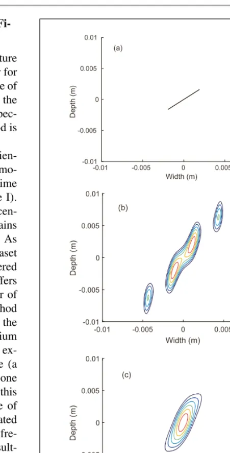
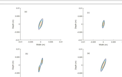
Figure 7 depicts reconstructions of a 5 mm crack orien-tated at 40◦ _{to the horizontal axis, embedded in a} homo-geneous medium, using FMC data generated by the time domain finite element method (see Section 3.1, Table I). Note that the sampling domain is a 20 mm2 _region cen-tered on the flaw (see Figures 3 and 4) and this remains constant for all reconstructions shown in this paper. As discussed in Section 3, only a subset of the FMC dataset (arising from the central 44 elements) has been considered in order to exclude scattering by the backwall. This offers an angular aperture of only 83◦_{, less than one quarter of} the full aperture (360◦_{) at which the Factorisation Method} performs optimally. No TSVD has been taken here as the flaw is embedded in a completely homogeneous medium and the null space of the scattering matrix already ex-ists. The image is plotted over a 6 dB dynamic range (a standard threshold for measuring defects larger than one wavelength) where the outermost contour is aligned to this limit. Figure 7a shows the known geometry and size of the defect. Image (b) depicts the reconstruction generated by applying the Factorisation Method to the single fre-quency (1.5 MHz) scattering matrix. Although the result-ing image is oversized (11.7 mm in length) and includes two lower amplitude artefacts, the method has identified the defect as a tilted ellipse-like scatterer. As discussed in Section 3, it is possible that improved reconstructions of the flaw may be achieved at different frequencies. How-ever, withouta prioriknowledge of the flaw’s dimensions, the optimal frequency cannot be deduced. Thus the multi-frequency approach was adopted to generate image (c) where scattering matrices were generated over the range 0.75 MHz–2.25 MHz, at intervals equal to the sampling frequencyfs, and then summed. Again, the result is a tilted

ellipse although this time the additional artifacts have dis-appeared and an improved crack length estimate of 9.6 mm is achieved.

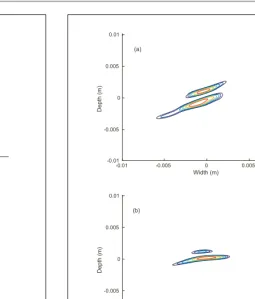
To further assess the suitability of the Factorisation Method for application in NDT, it has been applied to data arising from the FEM simulation of an ultrasonic wave scattered by a 5 mm crack of 40◦ _orientation (rela-tive to the horizontal axis) embedded in a heterogeneous medium (see Section 3.1 for details and Figure 7a for the defect size and geometry). Again, to exclude the signals where the ﬂaw scattering is conﬂated with that of the back wall, only the data arising from the central 44 array el-ements is considered (an angular aperture of only 83◦_). In Figure 8, results from application of the Factorisation Method to variants of the scattering matrix are plotted. Image (a) shows the reconstruction arising from the

sin--0.01 -0.005 0 0.005 0.01

Width (m) (a)

-0.01 -0.005 0 0.005

0.01

Depth

(m)

-0.01 -0.005 0 0.005 0.01 Width (m)

(b)

-0.01 -0.005 0 0.005 0.01

Depth

(m)

-0.01 -0.005 0 0.005 0.01 Width (m)

(c)

-0.01 -0.005 0 0.005 0.01

Depth

[image:8.595.270.496.52.496.2]

(m)

Figure 7. Crack reconstructions from FMC data arising from ﬁ-nite element simulation of the scattering of ultrasonic waves by a 5 mm crack with 40◦_{orientation embedded in a homogeneous} medium. Image (a) depicts the known defect size and geometry. This was reconstructed by (b) the Factorisation Method applied to the scattering matrix arising at 1.5 MHz and (c) the Factorisa-tion Method applied to the multi-frequency scattering matrix.

gle frequency (1.5 MHz), non regularised (m= 44) scat-tering matrix, measuring 7.3 mm. Image (b), demonstrates the result when only the ﬁrst four largest singular values are used to approximate a smoother single frequency scat-tering matrix at 1.5 MHz (m=4). Although the measure-ment is 9 mm, the method has correctly determined that we are dealing with a crack-like ﬂaw. Image (c) arises from the multi-frequency (spanning the range 0.75 MHz-2.25 MHz at intervals of fs), non-regularised (m = 44)

(9)

-0.01 -0.005 0 0.005 0.01 Width (m)

(a)

-0.01 -0.005 0 0.005 0.01

Depth

(m)

-0.01 -0.005 0 0.005 0.01 Width (m)

(b)

-0.01 -0.005 0 0.005 0.01

Depth

(m)

-0.01 -0.005 0 0.005 0.01 Width (m)

(c)

-0.01 -0.005 0 0.005 0.01

Depth

(m)

-0.01 -0.005 0 0.005 0.01 Width (m)

(a)

-0.01 -0.005 0 0.005 0.01

Depth

[image:9.595.25.502.55.358.2]

(m)

Figure 8. Crack reconstructions from FMC data arising from ﬁnite element simulation of the scattering of ultrasonic waves by a 5 mm crack with 40◦ _{orientation embedded in a heterogeneous medium by the Factorisation Method applied to (a) the scattering matrix} arising at 1.5 MHz, (b) the scattering matrix arising at 1.5 MHz regularised by the TSVD (m=10), (c) the multi-frequency scattering matrix and (d) the multi-frequency scattering matrix regularised by the TSVD (m=4).

image (d) is obtained which better represents the nature of the tilted crack defect. However, at the−6 dB thresh-old, the diameter of the reconstructed ﬂaw is 8 mm and its orientation is 69◦_{, both presenting signiﬁcant errors when} compared to the known 5 mm length and 50◦_orientation.

A final simulated dataset where a 2.5 mm diameter disc was embedded in the parent material to the left of the weld was also interrogated. Here data arising from the central 64 elements of the 128 element linear array was used to gen-erate the scattering matrices for inspection by the Factori-sation Method, affording an angular aperture of 112◦_{. The} exact defect geometry is shown in Figure 9 (a). Image (b) shows the results from interrogation of the scattering ma-trix arising at 2.25 MHz whilst image (c) arises from the multi-frequency scattering matrix generated over the fre-quency range 1.125 MHz-3.375 MHz. In this case, taking the TSVD of the scattering matrix inhibited the method’s ability to characterise the flaw. This can be attributed to the fact that the flaw is embedded in a homogeneous medium and since its scattering has been successfully isolated from that of the weld by limiting the aperture of inspection, taking the TSVD only serves to remove data relevant to the flaw. Additionally, the question of how many singu-lar values should be considered can be avoided (although we have a suggested a thresholding technique in Section 2.2, how to optimally truncate the SVD remains an open question). The diameters of the disc (measured along the longest dimension) are 3.4 mm and 2.8 mm respectively.

By using the multi-frequency scattering matrix, not only is the ﬂaw size estimate improved but a lower aspect ratio ellipse is yielded and thus the disc nature of the defect is better deﬁned.

(10)

-0.01 -0.005 0 0.005

Width (m) (a)

-0.01 -0.005 0 0.005

0.01

Depth

(m)

-0.01 -0.005 0 0.005 0.01 Width (m)

(b)

-0.01 -0.005 0 0.005 0.01

Depth

(m)

-0.01 -0.005 0 0.005 0.01 Width (m)

(c)

-0.01 -0.005 0 0.005 0.01

Depth

[image:10.595.58.496.52.420.2]

(m)

Figure 9. Reconstructions of a 2.5 mm diameter disc as shown in image (a) from FMC data arising from ﬁnite element simulation (see Table III) by the Factorisation Method applied to (b) the scattering matrix arising at 2.25 MHz and (c) the multi-frequency scattering matrix.

and 8d and 9c). This improved flaw identification comple-ments previous work on flaw classification [38, 39] where the primary objective is to distinguish between crack de-fects and volumetric scatterers.

3.3. Application to Experimental FMC Data

Figure 11 depicts reconstructions of the 3 mm disc from the experimental data as detailed in Table III. Once again, the aperture had to be cropped to exclude interference of the flaw scattering by that of the back wall and so the scattering matrix used arises from the central 64 elements placed directly above the flaw (again affording an angular aperture of 112◦_{). Image (a) shows the known defect size} and geometry, image (b) arises from application of the fac-torisation method to the single frequency scattering matrix

-0.01 -0.005 0 0.005

Width (m) (a)

-0.01 -0.005 0 0.005 0.01

Depth

(m)

-0.01 -0.005 0 0.005

Width (m) (b)

-0.01 -0.005 0 0.005 0.01

Depth

(m)

Figure 10. Reconstructions plotted at the−6 dB threshold of (a) the 5 mm crack embedded within the anisotropic steel weld and (b) the 2.5 mm diameter disc embedded to the left of the weld (see Tables I and II respectively) by the Total Focussing Method.

at 2.25 MHz and image (c) presents a similar reconstruc-tion, this time arising from the multi-frequency scattering matrix generated by summing over the range 1.125 MHz– 3.375 MHz at intervals equal to the sampling frequency,

fs. Note that the TSVD was not employed here as the ﬂaw

[image:10.595.29.305.54.491.2]

lies within the homogeneous parent material and so inter-ference by the microstructue does not dominate the scat-tering matrix. Measuring the defects along their longest dimension gives rise to defect measurements of 4 mm and 2.9 mm respectively.

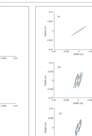
Figure 12 depicts reconstructions of the 7.8 mm crack from the experimental data as detailed in Table IV. Once again, the aperture had to be cropped to exclude interfer-ence of the flaw scattering by that of the back wall and so the scattering matrix used arises from the 42 elements placed directly above the flaw. This gives rise to an an-gular aperture of 122◦_{. Note that due to the close} prox-imity of the flaw to the backwall, it was not possible to entirely separate the scattering by the flaw from that of the backwall. Image (a) shows the known defect geome-try and size. Image (b) arises from the single frequency scattering matrix at 5 MHz and image (c) arises from the multi-frequency scattering matrix generated by summing over the range 2.5 MHz–7.5 MHz at intervals equal to the sampling frequency,fs. Measuring the defects along their

[image:10.595.241.497.56.355.2]

(11)

-0.01 -0.005 0 0.005 0.01 Width (m)

(a)

-0.01 -0.005 0 0.005

0.01

Depth

(m)

-0.01 -0.005 0 0.005 0.01 Width (m)

(b)

-0.01 -0.005 0 0.005 0.01

Depth

(m)

-0.01 -0.005 0 0.005 0.01 Width (m)

(c)

-0.01 -0.005 0 0.005 0.01

Depth

[image:11.595.192.495.50.497.2]

(m)

Figure 11. The geometry of the 3 mm diameter disc is plotted in (a). Reconstructions from FMC data arising from the phased ar-ray inspection of a steel block (see Table II) by the Factorisation Method applied to (b) the scattering matrix arising at 2.25 MHz and (b) the multi-frequency scattering matrix.

frequency is examined and an improved 10% error where multiple frequencies are considered. Furthermore, by us-ing the multi-frequency scatterus-ing matrix, the defect can be better identiﬁed as crack like than from the image aris-ing from the data at a saris-ingle frequency: the ratio of the crack length to crack width (which should be large) is ap-proximately 3.8 in the single frequency case, increasing to 5.2 in the multi-frequency case.

4. Conclusions

This paper has put forward a framework for using the Fac-torisation Method as a tool for ﬂaw characterisation in the ultrasonic NDT industry. A brief derivation was provided

-0.01 -0.005 0 0.005

Width (m) (a)

-0.01 -0.005 0 0.005 0.01

Depth

(m)

-0.01 -0.005 0 0.005 0.01 Width (m)

(b)

-0.01 -0.005 0 0.005 0.01

Depth

(m)

-0.01 -0.005 0 0.005 0.01 Width (m)

(c)

-0.01 -0.005 0 0.005 0.01

Depth

(m)

Figure 12. Reconstructions of the 7.8 mm crack orientated at 50◦ with respect to thex-axis shown in (a) from FMC data arising from the phased array inspection of welded austenitic plates (see Table IV) by the Factorisation Method applied to (b) the ing matrix arising at 5 MHz and (c) the multi-frequency scatter-ing matrix.

[image:11.595.32.428.51.512.2]

(12)

of the transducer array before a multi-frequency approach was adopted. In the case where the flaw was embedded in highly scattering medium it was shown that by using only a subset of the singular values, interference by noise could be minimised. Additionally, the method outperformed the standard imaging algorithm (the total focussing method, TFM) in sizing and differentiating between two different types of flaws: a volumetric side-drilled hole and an an-gled crack-like scatterer. The algorithm was applied to two experimental data sets, one in which a side-drilled hole lay next to a weld and the other where a lack-of-fusion crack lay on the boundary of the weld. In both cases, taking the TSVD inhibited the Factorisation Method’s performance (this can be attributed to the exclusion of valuable data). However, the multi-frequency approach yielded good flaw size estimates with errors of 0.1 mm for the 3 mm diameter side drilled hole and 0.7 mm for the 7.8 mm crack. And so, there remains much work to be done in order for the Fac-torisation Method to be adopted by end-users. However, this paper proposes a framework in which time domain, limited aperture data can be brought into the Factorisation Method domain. One natural direction to extend this work would be to consider the elastodynamic equations (rather than the Helmholtz equation). Also, it would be of interest to investigate the use of the Factorisation Method in the time-frequency domain [40].

Data Accessibility

The experimental data associated with this paper can be found at DOI:10.15129/60b6a5b8-e78e-4742-8414-aaba9399a9c8 and DOI:10.15129/086404bd-eb69-429b-978c-2c35cdbfcf87

Funding Statement

This work was funded through the UK Research Cen-tre in NDE Targetted Progra mme by the Engineering and Physical Sciences Research Council (grant number EP/I019731/1) and latterly the iNEED project (grant num-ber EP/P005268/1). Experimental samples were provided by Amec Foster Wheeler and Rolls Royce and software and support were supplied by Thornton-Tomasetti.

References

[1] B. W. Drinkwater, P.D. Wilcox: Ultrasonic Arrays for Non-destructive Evaluation: A Review. NDT & E Int39(2006) 525–541.

[2] C. Holmes, B. W. Drinkwater, P. D. Wilcox: Post Process-ing of the Full Matrix of Ultrasonic Transmit Receive Ar-ray Data for Non Destructive Evaluation. NDT & E Int38 (2005) 701–711.

[3] P. D. Wilcox, C. Holmes, B. W. Drinkwater: Advanced Re-ﬂector Characterisation with Ultrasonic Phased Arrays in NDE Applications. IEEE TUFFC54(2007) 1541–1549. [4] C. Li, D. Pain, B. W. Drinkwater, P. D. Wilcox: Imaging

Composite Material Using Ultrasonic Arrays. NDT & E Int 53(2013) 8–17.

[5] J. Zhang, B. W. Drinkwater, P. D. Wilcox, A. J. Hunter: De-fect Detection Using Ultrasonic Arrays: The Multi-Mode Total Focusing Method. NDT & E Int,43(2009) 123–133.

[6] J. Zhang, B. W. Drinkwater, P. D. Wilcox: The use of Ul-trasonic Arrays to Characterize Crack-like Defects. J. NDE 29(2010) 222–232.

[7] J. Zhang, B. W. Drinkwater, P. D. Wilcox: Defect Charac-terization Using an Ultrasonic Array to Measure the Scat-tering Coeﬃcient Matrix. IEEE TUFFC55(2008) 2254– 2265.

[8] K. M. M. Tant, A. J. Mulholland, A. Gachagan: A Model-Based Approach to Crack Sizing With Ultrasonic Arrays. IEEE TUFFC62(2015) 915–926.

[9] L. Bai, A. Velichko, B. Drinkwater: Ultrasonic characteri-zation of crack-like defects using scattering matrix similar-ity metrics. IEEE TUFFC62(2015) 545–559.

[10] A. Kirsch, N. Grinberg: The Factorisation Method for In-verse Problems. Oxford University Press, Oxford, 2008. [11] A. Kirsch: Characterisation of the Shape of a Scattering

Obstacle Using the Spectral Data of the Far Field Opera-tor. Inverse Problems14(1998) 1489–1512.

[12] A. Kirsch: Factorization of the Far-Field Operator for the Inhomogenous Medium Case and an Application in Inverse Scattering Theory. Inverse Problems15(1999) 413–429. [13] L. Bourgeois, E. Luneville: On the Use of Sampling

Meth-ods to Identify Cracks in Acoustic Waveguides. Inverse Problems28(2012) 105011.

[14] A. Kirsch: The MUSIC Algorithm and the Factorization Method in Inverse Scattering Theory for Inhomogenous Media. Inverse Problems18(2002) 1025–1040.

[15] C. Fan, M. Caleap, M. Pan, B. W. Drinkwater: A compar-ison between ultrasonic array beamforming and super res-olution imaging algorithms for non-destructive evaluation. Ultrasonics54(2014) 1842–1850.

[16] D. Colton, A. Kirsch: A Simple Method for Solving Inverse Problems in the Resonance Region. Inverse Problems12 (1996) 383–393.

[17] R. Potthast: A Survey on Sampling and Probe Methods for Inverse Problems. Inverse Problems222 (2006).

[18] M. Ikehata: Reconstruction of the Shape of the Inclusion by Boundary Measurements. Co mm. PDEs23(1998) 1459– 1474.

[19] R. Potthast: Stability Estimates and Reconstructions in In-verse Acoustic Scattering Using Singular Sources. J. Com-put. Appl. Math114(2000) 247–274.

[20] V. Baronian, L. Bourgeois, A. Recoquillay: Imaging an acoustic waveguide from surface data in the time domain. Wave Motion66(2016) 68–87.

[21] Q. Chen, H. Haddar, A. Lechleiter, P. Monk: A sampling method for inverse scattering in the time domain. Inverse Problems26(2010) 085001.

[22] N. Khaji, S. H. D. Manshadi: Time domain linear sampling method for qualitative identiﬁcation of buried cavities from elastodynamic over-determined boundary data. Computers & Structures153(2015) 36–48.

[23] C. D. Lines, S. N. Chandler-Wilde: A time domain point source method for inverse scattering by rough surfaces. Computing75(2005) 157–180.

[24] L. D. Russell, R. Potthast: The point source method for in-verse scattering in the time domain. Mathematical methods in the applied sciences29(2006) 1501–1521.

[25] A. Kirsch, S. Ritter: A linear sampling method for inverse scattering from an open arc. Inverse problems 16(2000) 89.

(13)

[27] Y. Boukari, H. Haddar: The Factorization method applied to cracks with impedance boundary conditions. Inverse Problems and Imaging.

[28] E. Kerbrat, C. Prada, D. Cassereau, M. Fink: Ultrasonic Nondestructive Testing of Scattering Media Using the De-composition of the Time-Reversal Operator. IEEE TUFFC 49(2002) 1103–1113.

[29] B. B. Guzina, F. Cakoni, C. Bellis: On the multi-frequency obstacle reconstruction via the linear sampling method. In-verse Problems26(2010) 125005.

[30] N. I. Grinberg: The Operator Factorization Method in In-verse Obstacle Scattering. IEOT54(2006) 333–348. [31] Y. A. Abramovich, C. D. Aliprantis: An invitation to

op-erator theory. Vol. 1. American Mathematical Soc., Rhode Island, USA, 2002.

[32] L. J. Cunningham, A. J. Mulholland, K. M. M. Tant, A. Gachagan, G. Harvey, C. Bird: The detection of ﬂaws in austenitic welds using the decomposition of the time-reversal operator. Proc. R. Soc. A472 No. 2188 (2016) 20150500.

[33] D. H. Chambers, A. K. Gautesen: Time reversal for a single spherical scatterer. JASA109(2001) 2616–2624.

[34] S. Shahjahan, F. Rupin, A. Aubry„ A. Derode: Evaluation of a multiple scattering ﬁlter to enhance defect detection in heterogeneous media. JASA141(2017) 624–640. [35] PZFlex, Thornton Tomasetti Defence Ltd. 6th Floor South,

39 St Vincent Place, Glasgow, Scotland, G1 2ER, United Kingdom.

[36] G. Harvey, A. Tweedie, C. Carpentier, P. Reynolds: Finite Element Analysis of Ultrasonic Phased Array Inspections on Anisotropic Welds. AIP Conf. Proc.1335(2010) 827– 834.

[37] I. Simonovski, L. Cizelj: Correlation length estimation in a polycrystalline material model. Proceedings of the Interna-tional Conference Nuclear Energy for New Europe. Bled, Slovenia, Sept. 2005.

[38] M. Kitahara, K. Nakahata, S. Hirose: Elastodynamic in-version for shape reconstruction and type classiﬁcation of ﬂaws. Wave Motion36(2002) 443–455.