CFD modelling of particle shrinkage in a fluidized bed for biomass fast pyrolysis with quadrature method of moment

CFD modelling of particle shrinkage in a fluidized bed for biomass fast

pyrolysis with quadrature method of moment

Bo Liua_{, Konstantinos Papadikis}b_{, Sai Gu}c_{, Beatriz Fidalgo}a_{, Philip Longhurst}a_{, Zhongyuan Li}a_and 3

Athanasios Koliosa 4

a - Bioenergy and Resource Management Centre, Energy Theme, Cranfield University, College Road, Cranfield, Bedfordshire MK43 0AL, UK; 5

b - Department of Civil Engineering, Xi’an Jiaotong Liverpool University, 111 Ren'ai Road, Suzhou Dushu Lake Science and Education 6

Innovation District, Suzhou Industrial Park, Suzhou 215123, China; 7

c - Department of Chemical & Process Engineering, University of Surrey, Guildford, Surrey GU2 7XH, UK 8

Abstract:

An Eulerian-Eulerian multi-phase CFD model was set up to simulate a lab-scale fluidized bed reactor 10

for the fast pyrolysis of biomass. Biomass particles and the bed material (sand) were considered to be 11

particulate phases and modelled using the kinetic theory of granular flow. A global, multi-stage 12

chemical kinetic mechanism was integrated into the main framework of the CFD model and employed 13

to account for the process of biomass devolatilization. A 3-parameter shrinkage model was used to 14

describe the variation in particle size due to biomass decomposition. This particle shrinkage model 15

was then used in combination with a quadrature method of moment (QMOM) to solve the particle 16

population balance equation (PBE). The evolution of biomass particle size in the fluidized bed was 17

obtained for several different patterns of particle shrinkage, which were represented by different 18

values of shrinkage factors. In addition, pore formation inside the biomass particle was simulated for 19

these shrinkage patterns, and thus, the density variation of biomass particles is taken into account. 20

Key words:

Fluidized bed, biomass, fast pyrolysis, CFD, QMOM, particle shrinkage 22

Fuel Processing Technology, Volume 164, September 2017, Pages 51-68 DOI:10.1016/j.fuproc.2017.04.012

Published by Elsevier. This is the Author Accepted Manuscript issued with: Creative Commons Attribution Non-Commercial No Derivatives License (CC:BY:NC:ND 4.0). The final published version (version of record) is available online at DOI:10.1016/j.fuproc.2017.04.012.

1. Background

Among the various forms of renewable energy, biomass is becoming a promising resource for energy 24

production, especially transportation fuel, as it has a huge potential for substituting fossil fuels on a 25

large scale. This would relieve the strong dependency of mankind on the petroleum industry and 26

contribute to tackling environmental problems, such as climate change and global warming. Biofuel 27

production is currently based mainly on edible crops, i.e. starch and sugar in the case of bioethanol, 28

and vegetable oils in the case of biodiesel. The use of food crops for the production of 1st_generation 29

biofuels may have negative effects on food production, including supply, prices and long term soil 30

depletion [1]. In contrast, lignocellulosic biomass such as energy crops, forestry and agricultural 31

residues, are a lower cost resource as these are not in direct competition with the food supply [2, 3]. 32

Therefore, advanced fuel technologies based on non-edible feed stocks are more attractive bio-33

based industry options for the future. 34

Bridgwater [4, 5] provides a comprehensive analysis of the thermal conversion of biomass from an 35

economic and technical perspective. Thermal treatment, particularly pyrolysis and gasification, is 36

potentially the most economic conversion process for producing biofuel in competition with oil-based 37

derivatives for storage and use in transportation [6, 7]. Of these methods, fast pyrolysis of 38

lignocellulosic biomass has considerable advantages for producing liquid bio-oil [8]. In the past two 39

decades, intensive research studies on fast pyrolysis have resulted in the design of a series of different 40

reactors such as ablative, auger, entrained flow, vacuum, rotating cone, bubbling fluidized bed and 41

circulating fluidized bed, etc. [9]. Among these developments, fluidized bed reactors have been proven 42

to have a high thermal efficiency and stable product quality as a result of their fast heating and 43

excellent gas-solid mass transfer rate [10]. 44

Biomass fast pyrolysis in a fluidized bed reactor is an extremely complex process as it involves a wide 45

range of chemical and physical phenomena across multiple scales of time and space. Typical examples 46

transfer and heterogeneous reactions [11]. Studying such complex processes not only requires the 48

chemical mechanism of pyrolysis to be determined from the molecular level, but importantly coupling 49

this with the gaseous and particulate flow environment. Understanding the behaviour of biomass 50

particles in a fluidized bed is central to determining the product distribution in order to optimize the 51

bio-oil quality [12]. With the rapid development of computing capability, the cutting-edge CFD 52

(Computational Fluid Dynamics) method becomes a good alternative to take the place of traditional 53

experiments in studying the massive flow and decomposition of particles in a fluidized bed reactor. 54

Whilst there are still problems and challenges for multi-phase flow in CFD, especially multi-physics 55

processes, CFD gives acceptable predictions about the hydrodynamic characteristics of the fluidized 56

bed [13-15]. Within the past ten years, effort has been placed on developing comprehensive, 57

computational and predictive CFD models for biomass pyrolysis within fluidized bed reactors. 58

According to differing views on particle dynamics in a CFD framework, existing models can be classified 59

into two basic categories: the Eulerian method and the Lagrangian method. Models in both categories 60

give successful predictions on the general properties of fast pyrolysis in a fluidized bed, such as particle 61

motion, heat transfer and mass transfer, as well as rate of biomass conversion and product yield [16]. 62

The Eulerian method is preferred by many researchers due to its low computing cost, good predictive 63

capability, and relative ease in computer programming. Hence, the Eulerian method has been widely 64

used in previous studies modelling fluidized bed reactors. Lathouwers and Bellan [17, 18] provide an 65

example of a comprehensive model based on Eulerian multi-phase fluid dynamics and the kinetic 66

theory of granular flow. They integrated the decomposition mechanism of biomass particles into their 67

CFD model to investigate the effects of operating parameters on product yields in a lab-scale fluidized 68

bed. Gerhauseret al.[19] carried out a more detailed modelling study focusing on the hydrodynamics 69

of the fluidized bed, whereas, Gerber et al. [20] set up an Eulerian-based model to simulate the 70

pyrolysis reactor with char particles as the fluidized medium so as to compare their numerical results 71

with experimental data. Xueet al.[21, 22] and Xue & Fox [12] developed a CFD model that accounts 72

loss of mass due to pyrolysis reactions making each particle more porous without changing its size. 74

Mellinet al.[23, 24] conducted a 3-D CFD simulation of a lab-scale fluidized bed and included a more 75

detailed prediction of gaseous and liquid product distribution by implementing a comprehensive 76

kinetic model of biomass pyrolysis proposed earlier by Ranziet al.[25]. In contrast to Eulerian method 77

examples, Fletcheret al.’s [26] work is based on the Lagrangian approach. In this study, the motion of 78

the biomass particle is tracked by applying Newton’s law, ignoring particle collision and employing a 79

global reaction mechanism to account for particle decomposition. Papadikiset al.[27-30] proposed a 80

method to simulate a single biomass particle in a pre-fluidized bed based on an Eulerian-Eulerian-81

Lagrangian CFD framework. The parameters of particle motion, heat transfer between the particle and 82

the bed medium, internal heat conduction and reaction, and particle shrinkage, were systematically 83

studied. Bruchmulleret al.[31] tracked 0.8 million red oak particles inside a pyrolysis fluidized bed 84

reactor with the Lagrangian method and validated their model with experimental results. 85

Although a number of relatively detailed CFD models which describe the complex gas-solid reactive 86

flow in a bubbling fluidized bed for biomass fast pyrolysis have been developed, none of them 87

completely addresses all the chemical and physical phenomena involved due to the complexity of the 88

system itself. In general, researchers have focused their attention on defining the motion of particles 89

and their transport processes rather than their physical change and therefore the properties of 90

biomass particles within CFD models, e.g. porosity, size, and shape. Despite this, it is known that 91

biomass particles’ changing size due to breakage and shrinkage occurs at high frequency during the 92

devolatilization process [18, 32-33, 34]. As a result, interactions between the biomass particle and the 93

bed medium are likely to change at the particle size and density changes. For example, the drag force 94

is directly affected, and consequently, the particle motion is likely to differ from cases where the size 95

and density changes are ignored; spatial distribution and the residence time of char particles in the 96

fluidized bed are also likely to be affected. The implication is that these changes are likely to impact 97

on secondary reaction sequences and the operating status of the reactor. It is this variation in size, 98

the devolatilization process. The phenomenon of biomass shrinkage during the pyrolysis process has 100

been studied by several researchers [34, 35, 36-37]. The most notable work among these is the 3-101

parameter shrinkage model proposed by Di Blasi. Despite this progress, the model can only be used 102

to predict the shrinkage of a single biomass particle at a given thermal condition but not the true 103

evolution of particle size in the complex reactor environment. Fan and Fox [13], Fanet al.[38, 39], 104

Marchisio & Fox [40] and Passalacqua et al. [41] propose a direct quadrature method of moment 105

(DQMOM) and combine this with the Eulerian multi-phase CFD model to describe the process of 106

particle mixing and segregation in a fluidized bed. Xue and Fox [12] further applied this method in 107

their CFD model to predict the distribution of biomass particle sizes in a bubbling fluidized bed during 108

fast pyrolysis. They argue that defining three quadrature abscissas guarantees a high accuracy in 109

determining the continuous particle size distribution; however, particle size variation was not taken 110

into account in this model. 111

In this paper, the Di Blasi 3-parameter particle shrinkage model is integrated into an Eulerian-based 112

multi-phase CFD framework in order to account for the evolution in particle size throughout the 113

fluidized bed. The quadrature method of moment (QMOM) is employed to solve the particle 114

population balance equation (PBE). This then determines the change in average particle diameter from 115

the biomass devolatilization. Differing shrinkage parameter values are used to represent differing 116

shrinkage patterns. These were investigated to find out how shrinkage affects the particle motion, 117

heating rate and the product yields. For the sake of simplicity, a multi-stage global kinetic model based 118

on pseudo-components was used to account for the chemical conversion of the biomass feed stock. 119

In addition to variation in particle size, the variation in density of the biomass was taken into account. 120

To best of our knowledge, no work similar to this has been reported that studies the size variation for 121

2. Mathematical modelling

2.1 Governing equations

The basic idea underpinning the Eulerian model as it is used for multi-phase granular flow is to 125

consider each phase, including the physical continuous and discrete phases, as interpenetrative fluids. 126

Momentum equation of the solid phase is then closured with the kinetic theory in terms of models to 127

calculate the solid viscosity and solid pressure. A detailed description of the multi-phase Eulerian 128

model and kinetic theory can be found elsewhere in the multi-phase flow literature [42]. Table 1 gives 129

a summary of the governing equations used in simulation of a fluidized bed reactor. Solid shear 130

viscosity usually contains three main contributions, i.e. the collision viscosity, kinetic viscosity and 131

frictional viscosity. In this study, collision viscosity is calculated according to Gidaspow et al.[43], 132

whilst kinetic viscosity is accounted for with the correlation of Syamlalet al.[44]. Frictional viscosity 133

is added due to high solid hold up and calculated with the model proposed by Schaeffer [45] using an 134

internal frictional angle of 55 [12]. The radial distribution functiong0,ssand the solid pressurepsare 135

calculated according to Lunet al. [46]. The restitution coefficientesstakes the value of 0.9. The solid 136

granular temperatureΘsis calculated with the correlation proposed by Syamlalet al.[44]. For multi-137

phase flow problems, momentum interactions between each pair of phases arises due to the drag 138

force, which contributes as a source termRi,jin the phase momentum equations. A widely used drag 139

model proposed by Gidaspow et al. [43] is employed to calculate the gas-solid phase interaction 140

coefficientKi,j. The Syamlal-O’Brien-Symmetric model [47] is then used to calculate the drag coefficient 141

between the biomass particles and the sand phase. 142

Table 1 Governing equations of the fluidized bed reactor based on Eulerian-Granular theory 143

Models and equations

Continuity

Gas

(

)

(

)

,

3 1 1

1 1 1 j 1 1 j 1

j 1 j 1

m m S

t

ε ρ _{ε ρ}

= ≠

∂ _{+ ∇⋅ = − +}

∂ u

∑

Solid (sand/biomass)

(

)

(

)

,

3 i i

i i i j i i j i

j 1 j i

m m S

t

ε ρ

ε ρ

= ≠

∂ _{+∇⋅ = − +}

Momentum Gas

(

)

(

)

,

3 1 1 1

1 1 1 1 1 1 1 j j 1 j 1 1 j 1 j 1 1

j 1 j 1

p m m g

t

ε ρ _{ε ρ ε τ ε ρ}

= ≠

∂ _{+ ∇⋅ = − ∇ ∇⋅ + + − +}

∂

∑

u _{u u + R u u}

(

)

1 1 1 1 1 1 1 1

2

I 3

τ =ε µ ∇ +∇_{u u}T − ε µ∇⋅_{u ;}

(

)

, ,

1 j=K1 j j− 1

R u u

Solid (sand/biomass)

(

)

(

)

,

3 i i i

i i i i i i i i j j i j i i j i j i i

j 1 j i

p p m m g

t

ε ρ _{ε ρ ε τ ε ρ}

= ≠

∂ _{+ ∇⋅ = − ∇ −∇ ∇⋅ + + − +}

∂

∑

u

u u + R u u

(

)

i i i i i i i i i

2

I 3

τ ε µ= ∇ +∇ +ε λ_ − µ_∇⋅

 

T

u u u i=2, 3; Ri j, =Ki j,

(

)

Solid shear viscosity µs = µs col, +µs kin, + µs fr,

Collision viscosity _, 2 _,

(

)

4

d g 1 e

5

Θ

µ ε ρ

π

= +

Kinetic viscosity

(

)

[

(

)(

)

]

, . ,

s s s s

s kin ss ss s 0 ss

ss d

1 0 4 1 e 3e 1 g

6 3 e

ε ρ Θ π

µ = + + − ε

−

Frictional viscosity ,

sin s s fr 2D p 2 I φ µ =

Solid bulk viscosity 4 _0,

(

)

s

s s sd gs ss ess

Θ λ ε ρ

π

= +

Radial distribution function

1 1/3 0, ,max 1 s ss s g ε ε − =







_



_

















Solid pressure ps=ε ρ Θs s s+2ρs

(

)

Granular temperature

(

)

(

)

(

)

(

)

3

:

2 t ρ ε Θs s s ρ ε Θs s s p Is τs s kΘs Θs γΘs ϕg s

∂

+ ∇ ⋅ = − + ∇ + ∇ ⋅ ∇ − +

∂

 

 

  u

Collision dissipation energy

(

)

0, 2 3/2 12 1

s

ss ss

s s s

s

e g

d

Θ

γ ρ ε Θ

π − =

Transfer of kinetic energy ϕg s, = −3Kg s,Θs

Species transport ,

(

)

(

)

(

)

N i i i p

i i i i q i i q i q i q _{j i i j} i i q

j 1

x

x D x m m S

t

ε ρ

ε ρ

ε

ε

= ∂

+∇⋅ = ∇⋅ ∇ +ℜ + − +

∂ u

∑

Energy

(

)

(

)

(

)

, , , ,

,

: 3

i i i

i i i i i i i i j i i j j i j i j i

j 1 j i

i i

h p

h Q m h m h

t t

T S

ε ρ _{ε ρ ε τ}

λ = ≠ ∂ _{+ ∇ ⋅ =} ∂ _{∇ + ⋅ + + −} ∂ ∂ + ∇ ⋅ ∇ +

∑

u + u R u

144

Note: Phase index i, j: 1 – gas phase; 2 - sand phase; 3 – biomass phase 145

Species transport equation and energy equation are solved based on each phase. Among all of the 146

energy sources, interphase heat transfer and the release of heat from chemical reactions are the most 147

significant energy sources from the fast pyrolysis of biomass in a fluidized bed. Table 2 gives the 148

thermodynamic parameters used in this work. Interphase heat transfer in a biomass fast pyrolysis 149

fluidized bed is extremely complex due to a variety of different physical heat transfer processes 150

transfer and radiative heat transfer. Thus far, no work has been done to account for all these heat 152

transfer processes in a single mathematical model. Most of the existing studies are concerned mainly 153

with the gas-solid heat transfer which is likely to be dominant in particle heating. In this study, the 154

conductive and radiative heat transfer effects of the sand phase are not taken into account. A well-155

known Nusselt correlation proposed by Gunn [48] was employed in this work to account for interphase 156

heat transfer between the fluidizing gas and the sand phase. Since the volumetric concentration of 157

the biomass phase is very low throughout the fluidized bed, existence of the biomass particles can be 158

ignored when calculating the gas-sand heat transfer coefficient. Heat transfer between the biomass 159

particles and the bed medium was calculated according to Collieret al.[49], who proposed a modified 160

Nusselt correlation in their studies on heat transfer between a free-moving bronze sphere and the 161

dense fluidizing medium (gas and inert particles). They argue that gas-solid heat transfer is dominant 162

when the heat transfer sphere is smaller than the bed particles, which is exactly the case in the current 163

study. 164

. .

. Re0 62( / )0 2 b s

Nu= +2 0 9 d d (1)

165

Where,dbis the diameter of the biomass particle;dsis the diameter of the sand particle. 166

Table 2 Thermodynamic parameters used in the simulation 167

Species Cp(kJ·kg-1·K-1) λ (W·m-1·K-1)

Cellulose, activated cellulose 2.3 [50] 0.2426 [50] Hemicellulose, activated hemicellulose 2.3 [50] 0.2426 [50] Lignin, activated lignin 2.3 [50] 0.2426 [50]

Char 1.1 [50] 0.1046 [51]

Tar 2.5 [50] 0.02577 [52]

Gas, void 1.1 [51] 0.02577 [51]

Nitrogen 1.091 [27] 0.0563 [27]

Sand 830 [24] 0.25 [24]

168

2.2 Chemical kinetic model of the biomass decomposition

Since this paper focuses mainly on demonstrating a method to describe the particle density 171

and size change in a fluidized bed reactor, rather than accurately predicting product yields, a 172

global chemical kinetic mechanism satisfies the current model in accounting for the biomass 173

devolatilization process. Shafizadeh and Bradbury [53] argue that, in the process of cellulose 174

pyrolysis, an activated intermediate is first produced, then two competitive conversion routes 175

occur afterwards, one which produces condensable bio-oil, and the other which gives 176

permanent gas and char. Ward and Braslaw [54], Koufopanoset al.[55], and Miller and Bellan 177

[56] extend this mechanism to the other main components of lignocellulosic biomass – 178

hemicellulose and lignin, and thus obtain a collective kinetic mechanism for biomass pyrolysis, 179

see Figure 1. 180

181

Fig. 1 A multi-stage global reaction mechanism of biomass fast pyrolysis 182

The biomass feedstock used in this work was assumed to be composed of 41wt.% cellulose, 183

32wt.% hemicellulose, and 27wt.% lignin. This is a typical woody biomass composition [57]. 184

Chemical reactions 1-4 from Figure 1 are first-order Arrhenius reactions with respect to the 185

corresponding reactant. The kinetic parameters are shown in Table 3, where Y value in 186

reaction 3 depends on the specific components. 187

Table 3 Kinetic parameters and reaction heat of biomass pyrolysis 188

Reaction Y A (s-1_{) E(kJ·mol}-1_{) kT=773K (kg·m}-3_·s-1_{) ∆h (kJ·kg}-1₎

k1,c 2.8×1019 242.4 539.246 [53] 0 [50]

k2,c 3.28×1014 196.5 8.775 [53] 255 [58]

k3,c 0.35 1.3×1010 150.5 0.5232 [53] -20 [58]

k1,h 2.1×1016 186.7 2670.041 [54] 0 [58]

k3,h 0.6 2.6×1011 145.7 22.450 [56] -20 [58]

k1,l 9.6×108 107.6 35.493 [54] 0 [58]

k2,l 1.5×109 143.8 0.175 [56] 255 [58]

k3,l 0.75 7.7×106 111.4 0.156 [56] -20 [58]

k4 4.28×106 108.0 0.147 [59] -42 [50]

Note: subscriptcrepresents cellulose;hrepresents hemicellulose;lrepresents lignin.

189

The continuous loss of particle mass from devolatilization makes the biomass particles shrink and 190

become more porous. Pore formation plays an important role in the apparent density change of the 191

biomass particle. It is assumed that pores which form inside the biomass particle fill with permanent 192

gas produced by the decomposition process. In other words, the majority of permanent gas produced 193

is released to the gas phase, and a small fraction remains in the biomass particle, forming pores. 194

Indeed, biomass particles maintain a very small holdup within the fluidized bed [21, 23], so the total 195

amount of permanent gas inside the pores is extremely small and can be ignored when compared with 196

the counterpart released to the gas phase. Therefore, this assumption incurs no significant artificial 197

errors and provides a simple way to account for the apparent density change. The apparent density 198

of the biomass particle is defined as the volume-weighted-average density of the component true 199

densities, including virgin biomass, activated biomass, char, and permanent gas in pores that 200

constitute the particle. 201

1 N

q apparent

q 1 q

x

ρ

ρ





= 

_



_



∑



202

Where,xqis the mass fraction of theqthcomponent in the biomass phase, which has exactly the same 203

meaning asx3,qin the species equation;ρq is the true density of theqthcomponent. All phases and 204

species involved in the current CFD model were numbered as shown in Table 4. Onlyn-1transport 205

equations were actually solved for each phase which containsnspecies in all. Thenth_{component mass} 206

fraction can be derived directly from the law of unity: , ,

n 1 i n i k

k 1

x

1

x

=

= −

∑

207

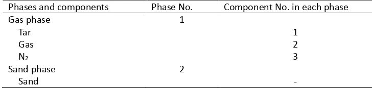
Table 4 Reference number of species in gas and biomass phase 208

Phases and components Phase No. Component No. in each phase Gas phase Tar Gas N2 1 1 2 3 Sand phase

-Biomass phase Char Activated-lignin Activated-hemicellulose Activated-cellulose Lignin Hemicellulose Cellulose Void Ash 3 1 2 3 4 5 6 7 8 9 209

Source termsRi,q referred to in the species transport equation can be calculated according to the 210

reaction mechanism and kinetic data provided in Figure 1 and Table 3, respectively. The numbering 211

criteria summarized in Table 4 are applied to subscriptsiandqin the species transport equation, and 212

the reaction source termRi,qfor each species can be written as follows. 213

Table 5 Source terms of the species transport equations due to chemical reactions 214

, , , , , , , ,

1 1 ρ ε3 3 2 c 3 4k x ρ ε3 3 2 h 3 3k x ρ ε3 3 2 lk x3 2 ρ ε1 1 4 1 1k x

ℜ = + + −

, , ( ) , , ( ) , , ( ) , ,

1 2 ρ ε3 3 3 ck 1 Y xc 3 4 ρ ε3 3 3 hk 1 Y xh 3 3 ρ ε3 3 3 lk 1 Y xl 3 2 ρ ε1 1 4 1 1k x

ℜ = − + − + − +

, , , , , , ,

3 1 ρ ε3 3 3 c c 3 4k Y x ρ ε3 3 3 h hk Y x3 3 ρ ε3 3 3 l lk Y x3 2

ℜ = + +

, , , , ,

3 2 ρ ε3 3 1 c 3 5k x ρ ε3 3 2 ck x3 2

ℜ = −

, , , , ,

3 3 ρ ε3 3 1 hk x3 6 ρ ε3 3 2 ck x3 3

ℜ = −

, , , , ,

3 4 ρ ε3 3 1 c 3 7k x ρ ε3 3 2 c 3 4k x

ℜ = −

, , ,

3 5 ρ ε3 3 1 lk x3 5

ℜ = −

, , ,

3 6 ρ ε3 3 1 h 3 6k x

ℜ = −

, , ,

3 7 ρ ε3 3 1 c 3 7k x

ℜ = −

215

It can be noted in Table 5 that none of the above expressions account for the mass fraction of the 216

component “void” which represents the quantity of pores formed in a devolatilizing biomass particle. 217

OnlyR1,2gives the total amount of permanent gas produced per unit volume per unit time, in place of 218

an exact distribution ratio for that released to the gas phase and that remaining in the solid particle. 219

Hence, an artificial interphase mass transfer term should be defined to account for the pore formation 220

rate. In the process of biomass fast pyrolysis, the pore formation rate depends on the rate at which 221

the biomass solid disappears because of the occurrence of heterogeneous reactions. This can be 222

inside a particle but also size change of the particle itself. Disappearance of the solid component in a 224

biomass particle is an overall result of decomposition reactions 2 and 3. This can be calculated from 225

the chemical kinetics, whilst calculation of the particle shrinking rate needs additional models. In this 226

work the 3-parameter shrinkage model proposed by Di Blasi [34] is used to account for the size change 227

of biomass particles during fast pyrolysis, described in detail in Section 2.4. 228

2.3 Quadrature Method of Moment (QMOM) for Particle Population Balance Equation

(PBE)

Population distribution of a particulate system can be described generally with a particle number 231

density function with respect to different particle properties called the “internal coordinates”, which 232

include particle size, shape and any other properties distinguishing the particles from one another. In 233

a fluidized bed, the number density is not only a function of these “internal coordinates”, but also of 234

“external coordinates”, including their spatial position and time. In order to integrate the particle 235

number density function to the current Eulerian multi-phase CFD framework, the conservation law for 236

a particle number with a specific property was applied to each control volume in the computational 237

domain. Since the only internal coordinate concerned in this study is the particle size, the PBE in an 238

Eulerian multi-phase flow framework can be written as in equation (3): 239

( )

( ) ( )

n L L

n L n L

t L t

∂ _{+∇⋅ = −} ∂ ∂ 

 

∂ u ∂ ∂  (3)

240

Where,n(L)is the number density function with respect to the particle sizeL. It can be seen clearly 241

that the above equation is a transient Eulerian equation with source terms. The term on the right hand 242

side of equation (3) denotes the source due to particle growth/shrinkage. In general, this equation 243

should include other source terms with respect to particle aggregation and fragmentation. Particle 244

aggregation hardly exists in a biomass fast pyrolysis fluidized bed; however, particle fragmentation 245

does occur. As far as we know, there have been no experimental methods developed to measure the 246

Hence, only the particle shrinkage have been taken into account and other particle processes have 248

been ignored in this work. 249

Solving equation (3) directly would be extremely time-consuming due to its additional dimension of 250

particle size distribution. Randolph and Larson [60] proposed an indirect method for PBE time 251

evolution by calculating several low order moments of the number density function to reduce the 252

dimensionality and then solve a set of moment conservation equations. Nevertheless, a closure 253

equation set cannot be derived without knowing the particle size distribution. Where complex particle 254

phenomena are taken into account, such as size-dependent growth, particle fragmentation and 255

aggregation, this is especially the case. McGraw [61] approximated these moments with the n-point 256

Gaussian quadrature and finally improved the closure of this method for a broader range of particle 257

events. Xue and Fox [12] claimed that three integral quadrature abscissas can produce acceptable 258

simulation results for the particle size evolution in a biomass fast pyrolysis fluidized bed, which means 259

that only the first six, low order moment conservation equations need to be solved. Hence, the PBE 260

equation (3) is replaced by the following moment conservation equation in this study. 261

(

)

s k s s

s k k k s s s s s

0

m d

m m m kd n d d d

t t t

ρ _ρ ρ _{ρ ρ} ∞

−

∂ _{+ ∇ ⋅ =} ∂ _{+ ⋅ ∇ −} ∂ 

 

∂ u ∂ u

∫

262

Where,mk denotes the moment ofkth order;n(ds)is the number density function with respect to 263

particle diameter, which has the same meaning asn(L)in equation (3). The zero order momentm0 264

represents the total particle number density, the second order momentm2is related to total particle 265

area, and the third order momentm3 relates to the total particle volume. However, based on the 266

definition of the moment, other low-order moments such asm1, m4andm5have no clear physical 267

meanings. 268

2.4 Di Blasi 3-parameter shrinkage model

Shrinkage of a biomass particle during the devolatilization process is very complex as it involves char 270

shrinkage of the char layer formed in a wood slap pyrolysis subjected to a radiation heat flux. The total 272

volume of a biomass particle was considered to be a sum of the pore volume occupied by a gaseous 273

substance plus the solid volume remaining (volume occupied by char, unreacted biomass, and partly-274

reacted biomass). Therefore, a shrinkage model with three shrinkage factors was proposed, withα,β, 275

γrepresenting different shrinkage contributions. 276

The volume occupied by the solid was assumed to decrease linearly with the biomass components 277

and to increase linearly with the char mass, as devolatilization takes place. The shrinkage factor α 278

reflects the density change of the solid residuals due to char formation, a value ofα between 0 and 1 279

represents no density increase and maximum density increase, respectively. 280

S W C

W0 W0 W0

V M M

V M M

α

= + (5)

281

Where,Vsis the current solid volume;VW0is the initial solid volume;MW is the current mass of the 282

remaining biomass solid;MW0is the initial mass of the biomass solid;MCis the current char mass. The 283

volume occupied by volatiles is composed of two contributions, the first due to the initial volume of 284

pores,Vg0, and the second due to a fractionβ of the volume left by the biomass solid as a consequence 285

of devolatilization,VW0 − Vs. 286

( )

g g 0 W 0 S

V =V +β V −V (6)

287

The initial volume of volatiles in a biomass particle may also decrease with the size change of the 288

particle, depending on a reaction progress factorη,η=MW/MW0, and shrinkage factorγ. 289

( )

g 0 gi gi

V =ηV + 1−η γV (7)

290

Where,Vgiis the initial value ofVg0before the devolatilization process happens, depending totally on 291

the initial porosity of the biomass particle. The initial porosity of the biomass was assumed to be 0.5 292

2.5 Integration of the particle shrinkage into the CFD model

The key point of introducing the Di Blasi 3-parameter particle shrinkage model into the current CFD 295

framework is to translate the particle shrinkage pattern represented by different shrinkage factors 296

into the apparent density calculation and volume evolution occupied by volatiles inside the biomass 297

particle. The apparent density of the biomass particle is defined as the volume-weighted average of 298

the components’ true densities according to equation (2). This can be considered further as the 299

volume-weighted average of the volatile (gaseous substances occupying the void) true density and the 300

solid (unreacted biomass and char) true density. The density of the volatile in pores is assumed to be 301

the same as that of the permanent gas in the gas phase, while the solid density depends on the value 302

of the shrinkage factorαin a specific shrinkage pattern. The volume-weighted mixing law is applied 303

to calculate the density of the remained solid substances and make it consistent with the value ofαin 304

a specific shrinkage pattern by assigning a proper value to the char density. 305

In fact, differingβandγvalues account for differing manners of volume evolution of the component 306

“void” in the biomass phase. By prescribing a set of these values, the mass transfer term between 307

“void” and permanent gas m_{1 3}2_, 8 can be defined, and then the species transport equations are finally

308

closed. The shrinking rate of the biomass particle is the sum of the shrinking effects contributed from 309

“void” and solid. Equation (6) gives a simple expression that the total particle volume shrinkage rate 310

R(volumetric decreasing rate of the biomass phase per unit volume of the flow domain) is a sum of 311

those corresponding to void and solid volume change, respectively. 312

g s

R = R + R (8)

313

The volume occupied by the biomass phase in an Eulerian control volume can be calculated with 314

Vb=εbV, whereVis the total volume of the control volume. The shrinking rate can then be written as 315

follows: 316

b

dV

RV

dt = − (9)

Let both sides of the above equation be divided byVb: 318

b

b b

1 dV RV

V dt = − V (10)

319

Substituting 3/

b b

V = N dπ 6 into equation (10) results into: 320

( )

b

d d

Rd

dt

= −

3

ε

321

Equation (11) gives the size-dependent particle shrinking rate, which is exactly the source term as it 322

appears in the moment conservation equations. Three different shrinkage patterns were investigated 323

in the current study, which were related to three sets of shrinkage factors, respectively (See Table 6). 324

Calculation of the volumetric shrinking rate,R, interphase mass transfer, m_{1 3}2_, 8, and char density is

325

different, depending on the selected shrinkage pattern. 326

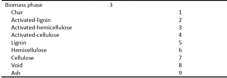
Table 6 Different shrinkage patterns 327

No shrinkage: α=1,β=1 andγ=1

char b b

1

ρ ρ ρ

α = =

(

)

2 8 3 3 2c 3c 3 6 3 3 2h 3h 3 7 3 3 2l 3l 3 8 void 1 3

biomass

void 3 3 3c c 3 6 3 3 3h h 3 7 3 3 3l l 3 8

char

m k k x k k x k k x

k Y x k Y x k Y x

ρ

ρ ε ρ ε ρ ε

ρ ρ

ρ ε ρ ε ρ ε

ρ

=_ + + + + + _

− + +

s g

R = R =0

Shrinkage pattern 1: α=1,β=0 andγ=1

char b b

1

ρ ρ ρ

α

= =

,

2 8

1 3

m =0

g

R =0

(

)

, , ,

, , ,

( ) ( ) ( )

s 3 3 2c 3c 3 6 3 3 2h 3h 3 7 3 3 2l 3l 3 8

biomass

3 3 3c c 3 6 3 3 3h h 3 7 3 3 3l l 3 8 char

1

R k k x k k x k k x

1

k Y x k Y x k Y x

ρ ε ρ ε ρ ε

ρ

ρ ε ρ ε ρ ε

ρ

=_ + + + + + _

− + +

Shrinkage pattern 2: α=0.5,β=0 andγ=0.5

char b b

1 2

ρ ρ ρ

α

= =

, , ,

, . ( ) ( ) ( )

2 8 void

g 1 3 3 3 2c 3c 3 6 3 3 2h 3h 3 7 3 3 2l 3l 3 8

biomass

R m 0 5 ρ ε k k x ρ ε k k x ρ ε k k x ρ

ρ

(

)

, , ,

, , ,

( ) ( ) ( )

s 3 3 2c 3c 3 6 3 3 2h 3h 3 7 3 3 2l 3l 3 8

biomass

3 3 3c c 3 6 3 3 3h h 3 7 3 3 3l l 3 8 char

1

R k k x k k x k k x

1

k Y x k Y x k Y x

ρ ε ρ ε ρ ε

ρ

ρ ε ρ ε ρ ε

ρ

=_ + + + + + _

− + +

328

In the case of the no shrinkage pattern, each shrinkage factor takes the value of unity. An artificial 329

mass transfer from the permanent gas to the “void” is required to compensate for the volume loss 330

due to biomass decomposition so that the particle size can remain constant. In the case of shrinkage 331

pattern 1, shrinkage factorβcomes to 0, and the other two factors stay the same as the above case. 332

This means that the “void” volume depends on the initial volume only, i.e. no artificial mass transfer 333

is needed. Particle size change, in this case, is attributed wholly to the net volume loss of the solid 334

substance. In the case of shrinkage pattern 2, the initial volume of the volatile varies with the reaction 335

progress. It is assumed that 50% of the initial volatiles leave the biomass particle as a consequence of 336

particle size decrease. So, an artificial mass transfer from the “void” to permanent gas needs to be 337

defined to account for this gaseous volume loss. It should be noted that, though the artificial mass 338

transfers introduced in the case of no shrinkage pattern and shrinkage pattern 2 are both between 339

permanent gas and the “void”, the mass transfer directions are the opposite. 340

3. Model setups and solution strategy

3.1 Model geometry and solution strategy

The geometrical model of the simulation in this study is based on a 300g/h lab-scale cylinder fluidized 343

bed reactor for biomass fast pyrolysis. Simulation was carried out using a 40mm×340mm 2-D 344

346

Fig. 2 The 2-D computational domain of the fluidized bed for numerical simulation 347

The phase-coupled SIMPLE algorithm was employed for pressure-velocity coupling. A volume of 348

fraction (VOF) equation was obtained for each solid phase from the total mass continuity. An explicit 349

variable arrangement was used for the VOF equation. Updating of the VOF at each iteration, was 350

included to achieve timely and better convergence, with a guarantee that the volume fraction of each 351

biomass phase matched the density updating. The volume fraction of the gas phase is obtained 352

directly from the law of unity. A second order upwind scheme was generally used in accounting for 353

the convection term discretization in the flow equation, energy equation, and species transport 354

equations. The three order upwind-like QUICK scheme was used for the VOF equations in order to 355

obtain high VOF precisions for each secondary phase. For temporal discretization, the first order 356

implicit method was employed. A relatively small time step length of 5×10-5_{s was used at the beginning} 357

of the simulation to overcome the difficulty of convergence due to poor initial fields, and a fixed time 358

3.2 Initial and boundary conditions

The biomass particles were assumed to be perfect spheres with a Sauter mean diameter of 325μm,

361

following a normal distribution for the particle size. Based on this size distribution, the low order 362

moments of the biomass feedstock were calculated, providing the boundary condition of the PBE at 363

the biomass inlet. Table 7 gives the 0th_-5th_{order moments of the size distribution.} 364

Table 7 Low order moments of the feed stock 365

Moments Calculation method

Moment-0

m

=

N

Moment-1 m1 = dm0

Moment-2 2 2 2

2 1 0

m = 2dm −d m +σ N

Moment-3 2 3

3 2 1 0

m =3dm −3d m +d m

Moment-4 2 3 4 4 4

4 3 2 1 0

m =4dm −6 d m +4d m −d m +3σ N

Moment-5 2 3 4 5

5 4 3 2 1 0

m =dm −10d m +10d m −5d m +d m

Where, N denotes the total particle number per unit volume of the feed stock;σ =0 3d. ; and d is the 366

number-mean diameter. Table 8 gives the specific values of these moments as well as other model 367

parameters. 368

Table 8 Model parameters and simulations conditions 369

Parameters Value

Biomass feeding rate (g/h) 180 (Equivalent to a cylinder experimental rig ) Nitrogen inflow velocity (m/s) 0.3

Minimum fluidized velocity (m/s) 0.081 Biomass feeding temperature (K) 300 Nitrogen feeding temperature (K) 773

Wall temperature (K) 773

Gas density (kg/m3_{) Incompressible ideal gas law}

Gas viscosity (Pa·s) 3.507×10-5_(773K)

Biomass particle size (μm) 325 (Sauter mean)

Initial moments of the biomass particle

Moment0 6.924×1010

Moment1 1.932×107

Moment2 5875

Moment3 1.910

Moment4 6.563×10-4

Moment5 2.366×10-7

Biomass component true density (kg/m3₎

Cellulose, hemicellulose, lignin 800 Char density for no shrinkage 800 Char density for shrink pattern 1 800 Char density for shrink pattern 2 1600

Biomass component initial mass fraction

Cellulose 4.094×10-1

Hemicellulose 3.195×10-1

Lignin 2.696×10-1

void 1.529×10-3

Biomass initial porosity (m3_{gas/ m}3_{particle) 0.5}

Biomass initial apparent density (kg/m3_{) 400}

Sand particle size (μm) 440

Sand density (kg/m3_{) 2500}

Sand initial packing height (mm) 80 Sand initial packing limit 0.63

370

3.3 Implementation of the simulation

In order to implement the simulation of the mathematical model depicted above, two additional 372

assumptions should be made. First, an even temperature distribution inside the biomass particle is 373

always achieved throughout the simulation; which means internal heat resistance is ignored. The 374

assumption is safe because of the low Bi number of the particle itself. Second, volatiles produced due 375

to the devolatization process are released instantaneously into the gas phase; which means 376

heterogeneous reactions play a dominant part in the interphase mass transfer process instead of 377

diffusion. This assumption is also safe because of the fairly small size of the biomass particle used in 378

this study. 379

The mathematical model of the fluidized bed was simulated with a widely used CFD package FLUENT 380

16.2. The interphase mass transfer between “void” and permanent gas, heat transfer between the 381

biomass phase and the bed medium, and source terms of the moment conservation equation due to 382

particle density and size variation, were accounted for by proper DEFINE MACROs of the FLUENT UDF 383

system. Each case in this study was run in parallel on an HPC cluster with 80 computing nodes, each 384

of which has two Intel E5-2660 CPUs, giving 16 CPU cores. Results gained from the simulation are 385

4. Results and discussion

4.1 Operational steady state of the fluidized bed

Since a mathematically rigorous steady state, in which all the field variables remain constants cannot 389

be reached in a fluidized bed, a transient solver is employed to carry out this kind of simulation. The 390

fluidized bed reactor reaches an operational steady state when the main field parameters reach fixed 391

values statistically at a specific time after the start-up. Not all of the field variables reach steady state 392

simultaneously for a single simulation process. Within this study, the hydrodynamics of the fluidized 393

bed seemed less sensitive to the initial field and achieved a steady state after a few seconds from the 394

beginning of the simulation. Typically, the biomass hold-up of the fluidized bed increased rapidly in 395

the first 5 seconds due to injection and reached an approximate constant value after 20 seconds, when 396

a steady output of the solid residue was set up. In contrast, the thermal steady state depends largely 397

on the initial temperature field. Xueet al.[21] observed that more than 100 seconds were required 398

to reach a thermal steady state when the initial temperature field deviated significantly from the final 399

temperature field, whereas if an appropriate initial temperature field is adopted, a thermal steady 400

state can be achieved in a few seconds. In this work, an initial temperature of 773K was used 401

throughout the fluidized bed to guarantee a rapid achievement of the thermal steady state. 402

4.2 Grid dependency test

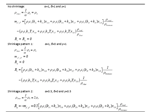
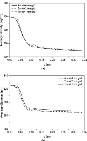
According to Minet al.[63], numerical simulations with a <4mm mesh can produce predictive results 404

of the main characteristics of a lab-scale fluidized bed. At the beginning of this work, a grid dependency 405

test were carried out with grid resolutions of 4mm, 2mm and 1mm. Results of some most interested 406

parameters of this study such as particle apparent density, particle diameter are plotted against 407

vertical axis of the fluidized bed reactor in Figure 3. Our test shows that all of the three grid resolutions 408

give very close results, especially for outlet values, and can be referred approximately as grid-409

independent solutions. Additionally, the 1mm and the 2mm grids seem to give better predictions than 410

Figure 3 (b). In balancing computational accuracy and efficiency, a uniform 2mm×2mm mesh was 412

finally adopted in this study. 413

0.00 0.05 0.10 0.15 0.20 0.25 0.30 0.35 100

200 300 400 500

A

ve

ra

ge

de

ns

ity

(k

g/

m

3 )

y (m)

4mmX4mm grid 2mmX2mm grid 1mmX1mm grid

414

(a)

415

0.00 0.05 0.10 0.15 0.20 0.25 0.30 0.35 260

280 300 320 340

A

ve

ra

g

e

d

ia

m

e

te

r

(

µ

m

)

y (m)

4mmX4mm grid 2mmX2mm grid 1mmX1mm grid

416

(b)

417

Fig. 3 Grid dependency test: (a) average density and (b) average particle size of the biomass 418

phase variation along the y axis at steady state (shrinkage pattern 1) 419

420

4.3 Density and size evolution of the biomass particles

Figure 4 (a) exhibits snapshots of the gas volume fraction distribution of the fluidized bed reactor 422

typical bubble formation, growth, rise, and breakage within the fluidized bed reactor. Solid particles 424

are firstly lifted up by the rising bubbles and then fall down due to density difference. These chaotic 425

motions of gas and solid particles largely enhance phase mixing, and heat and mass transfers. Cold 426

biomass particles are injected into the reactor and mix rapidly with the hot bed medium. As a result, 427

the volume fraction decreases by almost two orders of magnitude compared to the feeding state. This 428

occurrence can be observed in Figure 4 (b), which shows a snapshot of biomass volume fraction 429

distribution at 24s in the case of particle shrinkage pattern 1. The biomass phase cannot fill the whole 430

dense zone before entering the free board due to short particle residence time, which explains the 431

high concentration region adjacent to the feeding port. Because of the endothermic nature of the 432

decomposition reaction and low temperature of the feedstock (300K), an apparent temperature 433

gradient arises near the high concentration zone for the biomass phase (see Figure 5 (a)). 434

Devolatilization occurs inside the biomass particle when a certain temperature is reached. Pores are 435

formed as a consequence of continuous mass loss due to volatile release, which may result in a drop 436

in apparent density of the biomass particle. On the other hand, apparent density may increase due to 437

the increase in true densities of the solid components according to Di Blasi’s shrinkage theory, in which 438

the shrinkage factorα accounts mostly for true density variation of the solid with respect to solid 439

441

23.90s 23.95s 24.00s 24.05s 24.10s 24.00s

442

(a) (b)

443

Fig. 4 Snapshots of volume fraction distribution at steady state, shrinkage pattern 1: (a) 444

Gas phase; (b) biomass phase 445

446

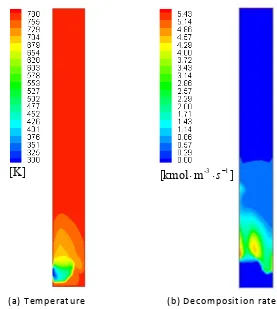
(a) Temperature (b) Decomposition rate

447

Fig. 5 (a) Distribution of temperature and (b) decomposition rate of the biomass phase in 448

the fluidized bed at 24s (data derived from shrinking pattern 1) 449

The apparent density distribution of the biomass phase in a fluidized bed is an overall result of particle 450

motion, heat transfer and heterogeneous reactions. Figure 6 shows the apparent density distribution 451

for biomass particles with different shrinking patterns at 24s. It can be observed that the particle 452

apparent density decreases throughout the vertical axis of the fluidized bed reactor in all of the three 453

shrinkage patterns. A sharp density gradient is observed close to the biomass injection point in the 454

dense zone of the fluidized bed. This is where devolatilization reactions occur intensively, see Figure 455

5 (b) – an example of reaction rate distribution at steady state. It is clear that the biomass particles 456

are heated rapidly in the dense zone and begin to reach the pyrolysis temperature at around 500K a 457

short distance away from the injection point. In the free board of the fluidized bed, the density 458

gradient of the biomass particle is much lower as most of the devolatilization reactions are finished in 459

the dense zone. In addition, the apparent density profile is different depending on the shrinkage 460

pattern. In the case of no shrinkage, the apparent density drops from 400 kg/m3_{at the inlet of the} 461

reactor to 95 kg/m3_{at the outlet. In the case of shrinkage patterns 1 and 2, the values at the outlet} 462

are 160 kg/m3_{and 245 kg/m}3_{, respectively. Obviously, the highest level of apparent density decrease} 463

appears in the case of no shrinkage pattern, then shrinkage pattern 1 and finally shrinkage pattern 2. 464

This is because biomass decomposition in the case of no shrinkage leads wholly to pore formation, 465

while in the other two cases particle size decrease is also the result of the biomass decomposition. 466

The apparent density of the biomass particle could actually increase and exceed the initial value of 467

400 kg/m3_{, if smaller values ofαandγwere used (for exampleα=0.2,γ=0.2). This is because smaller} 468

values of α and γ represent a larger degree of solid matrix reconstitution during the char formation

469

process and lesser degree of pore formation respectively, which is equivalent to a dominant 470

reconstitution of the solid matrix during the process of biomass pyrolysis. These results are not shown 471

here. 472

(

)

, ,

,

, =

x y apparent y t x

apparent y

2 1 x y

dVdt

t t dV

ε ρ

ρ

ε

∫∫

∫

474

(a) (b) (c)

475

Fig. 6 Apparent density distribution of the biomass particles inside the fluidized bed at 24s: 476

(a) no shrinkage pattern; (b) shrinkage pattern 1; (c) shrinkage pattern 2 477

0.00 0.05 0.10 0.15 0.20 0.25 0.30 0.35

0 100 200 300 400 500 600

No shrinkage Shrinking pattern 1 Shrinking pattern 2

A

ve

ra

ge

de

ns

ity

(k

g/

m

3 )

y (m) 478

Fig. 7 Spatial-temporal averaged density of the biomass particles in different shrinkage 479

patterns along the y axis 480

Figure 7 gives a statistical average result of the biomass density variation in the fluidized bed reactor 481

in terms of spatial-temporal averaged value along the y axis. The diagram was developed by calculating 482

-3

the volume-fraction-weighted mean density at each cross section of the fluidized bed and averaging 483

it over a period of time after steady state was finally achieved (see equation 12). Oscillations of the 484

stochastic instantaneous results were smoothed. These results give the apparent density evolution of 485

the biomass particles quantitatively in the fluidized bed and in good agreement with the phenomena 486

exhibited in Figure 6. 487

Particle size evolution for different shrinking patterns is illustrated in Figure 8. 0th_-5th _moment 488

conservation equations of the biomass phase were solved together with all other transport equations 489

synchronously; and the Sauter mean diameter of the biomass phase was derived fromm3/m2for every 490

control volume in the computational domain. As expected, particle size remained constant and equal 491

to the initial value at any point within the domain in the case of no shrinking pattern. In the case of 492

shrinking patterns 1 and 2, the particle size decreased related to the progress of the biomass 493

decomposition. Similarly to the apparent density, the highest gradient of particle shrinkage was 494

observed near the inlet area where the devolatilization and heterogeneous reactions mainly occur. It 495

was also observed that the temperature profile of the biomass phase was insensitive to different 496

shrinkage patterns in the current study. Figure 9 gives the spatial-temporal averaged temperatures of 497

the biomass phase along the y axis of the fluidized bed. It can be seen that curves representing 498

different shrinkage patterns overlap with each other in most parts of the reactor. Figure 10 gives the 499

spatial-temporal-averaged value of the biomass particle diameter along the y axis of the fluidized bed. 500

Simulation results show that the average diameter of the biomass particle drops to 290μm and 250μm

501

near the outlet of the fluidized bed for shrinking patterns 1 and 2, respectively. The pattern in which 502

a biomass particle shrinks not only depends on the physical properties of the particle itself, such as 503

size, shape, composition, structure, etc., but also on the surrounding heat and mass transfer 504

environment. Like some researchers in their work [28, 34], the shrinkage factors investigated in the 505

current study were given arbitrarily. To our knowledge, no current work gives an exact correlation 506

more on demonstrating a method to consider the particle shrinkage in a CFD simulation instead of 508

predicting an exact result for a real process. 509

510

(a) (b) (c)

511

Fig. 8 Size distribution of the biomass particles inside the fluidized bed at 24s: (a) no 512

shrinkage pattern; (b) shrinkage pattern 1; (c) shrinkage pattern 2 513

0.00 0.05 0.10 0.15 0.20 0.25 0.30 0.35

200 400 600 800 1000

No shrinkage Shrinking pattern 1 Shrinking pattern 2

A

ve

ra

g

e

te

m

pe

ra

tu

re

(K

)

y (m) 514

Fig.9 Spatial-temporal averaged temperature of the biomass particles in different shrinkage 515

patterns along the y axis 516

0.00 0.05 0.10 0.15 0.20 0.25 0.30 0.35 220

240 260 280 300 320 340 360

No shrinkage Shrinking pattern 1 Shrinking pattern 2

A

ve

ra

ge

di

a

m

et

e

r

(

µ

m

)

y (m) 517

Fig. 10 Spatial-time averaged diameter of the biomass particles in different shrinkage 518

patterns along the y axis 519

520

4.4 Particle tracking in an Eulerian CFD framework

Knowledge of particle motion is of great importance for the design of fluidized bed reactors, since it 522

can help to optimize the reactor configuration and choose reasonable operating conditions. In general, 523

two methods are used to simulate particle laden flows in a fluidized bed reactor, the Eulerian-granular 524

model and the Discrete Element Method DEM-CFD model. The latter is more suitable for particle 525

trajectory calculation as the complex fluid-particle and particle-particle interactions are investigated 526

by tracking a great number of ‘real’ particles individually; however, this method is extremely 527

computational expensive. In contrast, the computing cost of the Eulerian-granular method is much 528

lower because the particles are considered as a continuum, and particle-particle and particle-fluid 529

interactions are accounted for by means of solid viscosity closured by the granular kinetic theory and 530

drag force models, respectively. Particle tracking is also possible under the Eulerian-granular 531

framework, which is referred as the ‘fictitious tracer particle’ concept proposed by Liu and Chen [64]. 532

The concept of massless particle, routinely used by many researchers [65-67], is based on the 533

field. The tracer velocity can be either assigned by the local velocity of the nearest cell or extracted 535

with high-order numerical schemes [68-70]. Each fictitious tracer particle can be laid in an interested 536

computational cell at a specific physical simulation time and fully follow the movement of the solid 537

phase. The tracer particle is massless and the velocity is assigned by the solid phase velocity of the cell 538

where the tracer particle is located. Thus, the displacement of the tracer particle can be calculated 539

after a time interval, and a new position of the particle is then obtained. When this procedure is 540

repeated within each time step during the simulation, the trajectory of each tracer particle is obtained. 541

Although this is not a rigorous particle tracking technology based on ‘real’ particles, some important 542

particle motion information can be obtained. Forces exerted on the tracer particle, such as fiction and 543

collision, are implied in the solid phase motion accounted for by the kinetic theory. 544

545

(a) (b)

546 547

Fig. 11 (a) The biomass volume fraction and (b) comparison of the particle trajectories in 548

the fluidized bed at 24s (no shrinkage pattern) 549

Solid and vapour residence time are also parameters of great importance for a biomass pyrolysis 550

distribution, secondary reaction occurrence, etc. Vapour residence time can be estimated by means 552

of the superficial velocity of the fluidized gas and the gas phase effective volume in the fluidized bed. 553

However, solid residence time cannot be estimated in this way, since particles shrink and flow back 554

far more frequently than in the gaseous phase. In order to estimate the solid residence time of the 555

fluidized bed, ‘fictitious tracer particle’ concept was applied in this work. Massless tracer particles 556

were released one by one at different positions near the biomass inlet for every 50 time steps and 557

tracked in accordance with the transient update of the flow field. The velocity of an individual tracer 558

particle is assigned by the local velocity of the biomass phase at the control volume where the particle 559

is currently located. If the tracer particle moves and touches the walls, a full elastic reflection happens 560

so that a continuous particle trajectory can be obtained until the particle leaves the domain from the 561

top outlet. Most of the particles leave the domain after a certain period of tracking. However, a few 562

may be trapped permanently because zero-velocity regions exist at the two sides close to the outlet 563

of the fluidized bed. In addition to residence time, other particle information can be recorded 564

dynamically with this tracking technology. Any of the parameters of interest can be stored in a data 565

matrix when implementing the tracking process, similarly to that of storing the position information, 566

such as particle temperature, local sand volume fraction, etc. Some statistically averaged 567

characteristics of the biomass phase behaviour can be obtained by tracking a large number of 568

individual particles in a fluidized bed. Figure 11 gives a comparison of biomass volume fractions 569

alongside a number of particle trajectories. It can be observed that regions with dense particle 570

trajectories correspond accordingly with high volume fractions derived from the VOF equation. 571

Particles entering the domain with a low initial velocity from the inlet are unlikely to spread 572

immediately across a wide range within the fluidized bed medium. Instead, most of them travel along 573

the side wall to the top of the dense zone until reaching the splashing zone where more intensive 574

mixing happens due to bubble breakage; hence particles spread faster throughout the whole splashing 575

577

(a) (b) (c)

578

Fig. 12 Typical particle trajectories of the biomass particle in different shrinking pattern: (a) 579

no shrinkage pattern; (b) shrinkage pattern 1; (c) shrinkage pattern 2 580

Differences in the biomass particle motion inside the fluidized bed due to the implementation of a 581

different particle shrinkage pattern can be observed by means of the trajectories of the particles. 582

Figure 12 shows typical particle trajectories for different shrinkage patterns. It can be seen that, when 583

no shrinkage pattern is considered, most of the particles are likely to escape the splashing zone into 584

the free board without significant flow back (such as the red, blue and green lines in Figure 12(a)). 585

Nevertheless, some of the particles cannot directly escape the splashing zone and stay for some time 586

before entering the free board area (cyan and purple lines in Figure 12(a)). In the case of shrinkage 587

pattern 1, the flow back of the particles in the splashing zone and the area immediately after this zone 588

is more frequent. This may be related to the higher particle density which seems then to have a higher 589

influence on the particle motion than that of the particle size. In the case of particle shrinkage pattern 590

2, few particles escape the splashing zone directly. Most are trapped in the splashing zone for different 591