Supplementary Material:
Emulation of utility functions over a set of
permutations: sequencing reliability growth tasks
July 10, 2017
1
Proof of Proposition 1
The possible values of Kendall’s tau distance between any two permutations of length R are 0,1, . . . , T, where T = R(R−1)/2. Suppose we order the sequences from highest expected utility to lowest expected utility and, without loss of generality, suppose the ordering is denoted (1,2, . . . , R). We name this the base ordering of the sequences.
We can find the total number of permutations, CR,δ, which are at most distance δ from the base ordering. The Kendall’s tau distance to the base ordering is the number of pairs ofj, j0 such thatj < j0 but j0 appears before
j in the permutation. Any pair j, j0 which has this property is known as an inversion. Any permutation of the base ordering is a permutation of 1, . . . , R−1 withRinserted. If we insert Rat position l, this creates R−l new inversions. Thus the previous permutation must have had at mostδ−(R−l) inversions. Thus,
CR,δ =
δ
X
l=max(1,R−δ)
CR−1,δ+R−l,
= δ
X
l=δ−R+1
CR−1,l.
From this, we can calculate the number of permutations of the base ordering with a Kendall’s tau distance of δ as NR,δ = CR,δ−CR,dδ−1. Now, we are
be the second element isNR−1,δ−1 and the number of ways it can be them’th
element isNR−1,δ−m+1. The proportions in each case are given by dividing by
the number of permutations with Kendall’s tau distanceδ,NR,δ. This gives the result.
2
Proof of Proposition 2
The probability that the optimal sequence is in themcandidates, from Corollary 1, is
M
X
m=1
CR−2,δ−m+1
CR−1,δ
.
Clearly,CR−2,0 = 1 and δ−m+ 1≥0∀m = 1, . . . , M. Specifically, δ−M +
1 ≥ 0 and so M ≤ δ+ 1. Since the optimal sequence must be one of the R
permutations,
δ+1
X
m=1
CR−2,δ−m+1
CR−1,δ = 1
and
δ
X
m=1
CR−2,δ−m+1
CR−1,δ
= 1− 1
CR−1,δ
.
3
Prior expectation of the reliability under planned
development tasks
Following some development tasks, the system reliability, assuming that every fault found is corrected without introducing further faults, is given by
R(t,z) = I
Y
i=1
Ri(t)I[zi>di]
= I
Y
i=1
Ri(t)zi(1−di)
= I
Y
i=1
{1−zi(1−di)[1−Ri(t)]},
Z= (Z1, . . . , ZI)
0
andD= (D1, . . . , DI)
0
,
EZ|D[R(t,z)] = EZ|D
" I Y
i=1
{1−zi(1−di)[1−Ri(t)]}
#
= I
Y
i=1
EZi|Di[{1−zi(1−di)[1−Ri(t)]}]
= I
Y
i=1
EZi|Di
h
˜
R(t, zi, di)
i
,
asZi|Di is independent ofZj |Dj. Taking the expectation with respect toD, gives
ED
EZ|D[R(t,z)] =
I
Y
i=1
EDinEZi|Di
h
˜
R(t, zi, di)
io
.
We can express the expectation concerning faultias
EDinEZi|Di
h
˜
R(t, zi, di)
io
= Pr(Di = 1)
h
Pr(Zi= 1|Di = 1) ˜R(t,1,1)
+ Pr(Zi= 0|Di= 1) ˜R(t,0,1)
i
+ Pr(Di= 0)
h
Pr(Zi= 1|Di= 0) ˜R(t,1,0)
+ Pr(Zi = 0|Di= 0) ˜R(t,0,0)
i
. (1)
We can evaluate each of the quantities in this expression. They are
Pr(Di= 0) = 1−λi
1−
J
Y
j=1
(1−pi,j)κj
, Pr(Di= 1) =λi
1−
J
Y
j=1
(1−pi,j)κj
,
for the unconditional probabilities,
Pr(Zi= 1|Di= 0) =
λiQ J
j=1(1−pi,j)
κj
1−λi
h
1−QJ
j=1(1−pi,j)κj
i, Pr(Zi= 1|Di= 1) = 1
Pr(Zi= 0|Di= 0) =
1−λi 1−λi
h
1−QJ
j=1(1−pi,j)κj
for the conditional probabilities, ˜R(t,1,1) = ˜R(t,0,1) = ˜R(t,0,0) = 1 and ˜
R(t,1,0) =Ri(t). Thus the expectation in (1) is
λi
1−
J
Y
j=1
(1−pi,j)κj
[1×1 + 0×1]
+
1−λi
1−
J
Y
j=1
(1−pi,j)κj
λiQJj=1(1−pi,j)κj
1−λih1−QJ
j=1(1−pi,j)κj
iRi(t) +
1−λi
1−λih1−QJ
j=1(1−pi,j)κj
i×1
=λi−λi J
Y
j=1
(1−pi,j)κj+λi J
Y
j=1
(1−pi,j)κjRi(t) + 1−λi
= 1−λi(1−Ri(t)) J
Y
j=1
(1−pi,j)κj.
Substituting this into the expectation of interest, gives the result:
EZ|D[R(t,z)] = I
Y
i=1
1−λi(1−Ri(t)) J
Y
j=1
(1−pi,j)κj
4
Example of theoretical results
Suppose that there are 3 tasks which we wish to sequence. This means that there are 3! = 6 possible sequences of the 3 tasks. Define the value of the surrogate function for sequence xi to be fi = f(xi) and the expected utility to beui=U(xi), for i= 1, . . . ,6. Suppose that the ordering of the sequences using the surrogate function is f1 > f2 > f3 > f4 > f5 > f6, and that the
Kendall’s tau distance between the expected utility and the surrogate function is 2. This means thatτ = 11/15.
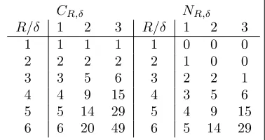
We can calculate the values ofCR,δandNR,δforR= 1, . . . ,6 andδ= 1,2,3, which will allow us to find the probability that the sequence with the maximum expected utility is in the highestM places ordered by surrogate function. The values are in Table 1.
CR,δ NR,δ
R/δ 1 2 3 R/δ 1 2 3
1 1 1 1 1 0 0 0
2 2 2 2 2 1 0 0
3 3 5 6 3 2 2 1
4 4 9 15 4 3 5 6
5 5 14 29 5 4 9 15
[image:4.612.212.401.505.605.2]6 6 20 49 6 5 14 29
Table 1: Tables showing the values of CR,δ and NR,δ for R = 1, . . . ,6 and
δ= 1,2,3.
C4,0= 1. Therefore, the probabilities that the sequence with highest expected
utility is in the sequences with the highestM values off(·), forM = 1, . . . ,6 are (9/14,13/14,14/14,14/14,14/14,14/14), respectively. We see that, choosing
M =δ+ 1 = 3, we obtain the optimal sequence with probability 1 as shown by Proposition 2 in the main paper.
In this simple case we can find the probabilities directly. There are 6! = 720 possible orderings of the expected utilitiesu1, . . . , u6. Of these, 14 have a
Kendall correlation τ = 11/15 with the surrogate function ordered as above. Suppose that the true ordering of the expected utilities is some permutation of
u1, . . . , u6, say u(1) < u(2) < u(3) < u(4) < u(5) < u(6). Then the orderings
below of the sequences have the required Kendall correlation (given in order, from first to last).
We see that, of the 14 sequences, in 9 cases the sequence with the highest value for the expected utility is in the first position in the ordering (red), in 4 cases it is in the second position (blue) and in one case it is in the third position. This results in the probabilities given above.
u(1), u(2), u(3), u(5), u(6), u(4) u(1), u(2), u(3), u(6), u(4), u(5) u(1), u(2), u(4), u(3), u(6), u(5) u(1), u(2), u(4), u(5), u(3), u(6) u(1), u(2), u(5), u(3), u(4), u(6) u(1), u(3), u(2), u(4), u(6), u(5) u(1), u(3), u(2), u(5), u(4), u(6) u(1), u(3), u(4), u(2), u(5), u(6) u(1), u(4), u(2), u(3), u(5), u(6) u(2), u(1), u(3), u(4), u(6), u(5)
u(2), u(1), u(3), u(5), u(4), u(6) u(2), u(1), u(4), u(3), u(5), u(6)
u(2), u(3), u(1), u(4), u(5), u(6) u(3), u(1), u(2), u(4), u(5), u(6)
5
Splitting the training sample: an illustrative
example
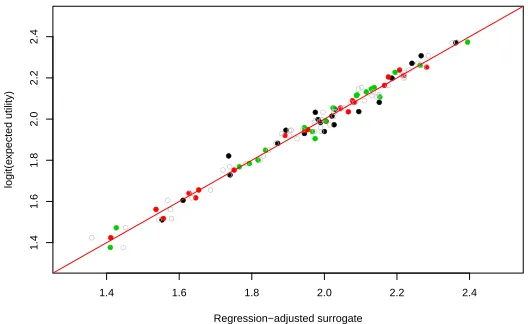
In the illustrative example of Section 4 in the main paper, we have a training sample of sizeN = 60. Here we split this training sample intos= 3 sub-samples of size 20 and fit a regression-adjusted surrogate (using the Benter-Pearson model-correlation combination) to each. Figure 1 plots the logit-transformed expected utilities against the fitted values from the regression-adjusted emu-lators in each of the sub-samples. For comparison, Figure 1 also contains the fitted values from the regression-adjusted surrogate based on allN= 60 training samples.
It can be seen that there is a good correspondence between the emulator values based on the sub-samples and the emulator values based on the full training sample, as we would expect.
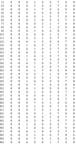
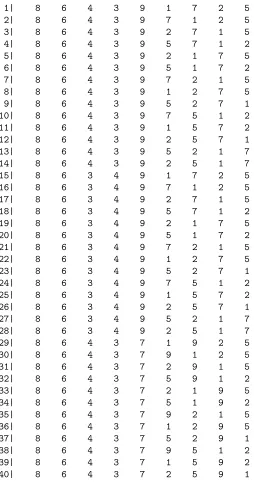
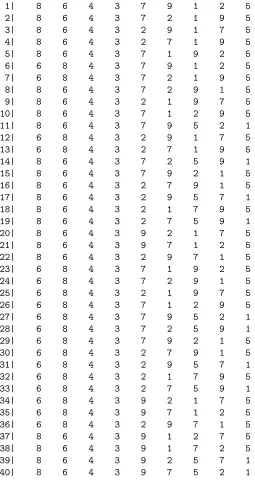
We can also look at the topM sequences under each sub-sample-based em-ulator and compare with theM sequences under the emulator based on the full training sample. These are shown in Tables 2 to 5.
1| 6 8 4 1 3 2 7 5 9
2| 6 8 4 1 2 3 7 5 9
3| 6 8 4 1 7 3 2 5 9
4| 6 8 4 1 5 3 2 7 9
5| 6 8 4 3 1 2 7 5 9
6| 6 8 4 1 9 3 2 7 5
7| 6 8 4 3 2 1 7 5 9
8| 6 8 4 3 7 1 2 5 9
9| 6 8 4 1 3 2 5 7 9
10| 6 8 4 3 5 1 2 7 9
11| 6 8 4 2 1 3 7 5 9
12| 6 8 4 1 2 3 5 7 9
13| 6 8 1 4 3 2 7 5 9
14| 8 6 4 1 3 2 7 5 9
15| 6 8 4 2 3 1 7 5 9
16| 6 8 1 4 2 3 7 5 9
17| 6 8 1 4 7 3 2 5 9
18| 6 8 4 1 5 3 7 2 9
19| 8 6 4 1 2 3 7 5 9
20| 8 6 4 1 7 3 2 5 9
21| 6 8 4 2 7 1 3 5 9
22| 6 8 4 2 5 1 3 7 9
23| 6 8 1 4 5 3 2 7 9
24| 6 8 4 7 1 3 2 5 9
25| 6 8 4 1 9 3 2 5 7
26| 8 6 4 1 5 3 2 7 9
27| 6 8 4 3 9 1 2 7 5
28| 6 8 4 3 1 2 5 7 9
29| 6 8 4 7 3 1 2 5 9
30| 6 8 4 1 9 3 7 2 5
31| 6 8 4 7 2 1 3 5 9
32| 8 6 4 3 1 2 7 5 9
33| 6 8 4 3 2 1 5 7 9
34| 6 8 4 2 9 1 3 7 5
35| 6 8 1 4 9 3 2 7 5
36| 6 8 1 3 4 2 7 5 9
37| 8 6 4 1 9 3 2 7 5
38| 6 8 4 1 3 2 7 9 5
39| 6 8 4 7 5 1 3 2 9
[image:6.612.177.431.136.622.2]40| 6 8 4 3 5 1 7 2 9
1| 8 6 4 3 9 1 7 2 5
2| 8 6 4 3 9 7 1 2 5
3| 8 6 4 3 9 2 7 1 5
4| 8 6 4 3 9 5 7 1 2
5| 8 6 4 3 9 2 1 7 5
6| 8 6 4 3 9 5 1 7 2
7| 8 6 4 3 9 7 2 1 5
8| 8 6 4 3 9 1 2 7 5
9| 8 6 4 3 9 5 2 7 1
10| 8 6 4 3 9 7 5 1 2
11| 8 6 4 3 9 1 5 7 2
12| 8 6 4 3 9 2 5 7 1
13| 8 6 4 3 9 5 2 1 7
14| 8 6 4 3 9 2 5 1 7
15| 8 6 3 4 9 1 7 2 5
16| 8 6 3 4 9 7 1 2 5
17| 8 6 3 4 9 2 7 1 5
18| 8 6 3 4 9 5 7 1 2
19| 8 6 3 4 9 2 1 7 5
20| 8 6 3 4 9 5 1 7 2
21| 8 6 3 4 9 7 2 1 5
22| 8 6 3 4 9 1 2 7 5
23| 8 6 3 4 9 5 2 7 1
24| 8 6 3 4 9 7 5 1 2
25| 8 6 3 4 9 1 5 7 2
26| 8 6 3 4 9 2 5 7 1
27| 8 6 3 4 9 5 2 1 7
28| 8 6 3 4 9 2 5 1 7
29| 8 6 4 3 7 1 9 2 5
30| 8 6 4 3 7 9 1 2 5
31| 8 6 4 3 7 2 9 1 5
32| 8 6 4 3 7 5 9 1 2
33| 8 6 4 3 7 2 1 9 5
34| 8 6 4 3 7 5 1 9 2
35| 8 6 4 3 7 9 2 1 5
36| 8 6 4 3 7 1 2 9 5
37| 8 6 4 3 7 5 2 9 1
38| 8 6 4 3 7 9 5 1 2
39| 8 6 4 3 7 1 5 9 2
[image:7.612.177.431.135.622.2]40| 8 6 4 3 7 2 5 9 1
1| 8 6 4 3 7 9 1 2 5
2| 8 6 4 3 7 2 1 9 5
3| 8 6 4 3 2 9 1 7 5
4| 8 6 4 3 2 7 1 9 5
5| 8 6 4 3 7 1 9 2 5
6| 6 8 4 3 7 9 1 2 5
7| 6 8 4 3 7 2 1 9 5
8| 8 6 4 3 7 2 9 1 5
9| 8 6 4 3 2 1 9 7 5
10| 8 6 4 3 7 1 2 9 5
11| 8 6 4 3 7 9 5 2 1
12| 6 8 4 3 2 9 1 7 5
13| 6 8 4 3 2 7 1 9 5
14| 8 6 4 3 7 2 5 9 1
15| 8 6 4 3 7 9 2 1 5
16| 8 6 4 3 2 7 9 1 5
17| 8 6 4 3 2 9 5 7 1
18| 8 6 4 3 2 1 7 9 5
19| 8 6 4 3 2 7 5 9 1
20| 8 6 4 3 9 2 1 7 5
21| 8 6 4 3 9 7 1 2 5
22| 8 6 4 3 2 9 7 1 5
23| 6 8 4 3 7 1 9 2 5
24| 6 8 4 3 7 2 9 1 5
25| 6 8 4 3 2 1 9 7 5
26| 6 8 4 3 7 1 2 9 5
27| 6 8 4 3 7 9 5 2 1
28| 6 8 4 3 7 2 5 9 1
29| 6 8 4 3 7 9 2 1 5
30| 6 8 4 3 2 7 9 1 5
31| 6 8 4 3 2 9 5 7 1
32| 6 8 4 3 2 1 7 9 5
33| 6 8 4 3 2 7 5 9 1
34| 6 8 4 3 9 2 1 7 5
35| 6 8 4 3 9 7 1 2 5
36| 6 8 4 3 2 9 7 1 5
37| 8 6 4 3 9 1 2 7 5
38| 8 6 4 3 9 1 7 2 5
39| 8 6 4 3 9 2 5 7 1
[image:8.612.176.431.137.622.2]40| 8 6 4 3 9 7 5 2 1
1| 8 6 4 3 1 7 2 9 5
2| 8 6 4 3 1 7 9 2 5
3| 8 6 4 3 7 1 2 9 5
4| 8 6 4 3 7 1 9 2 5
5| 8 6 4 3 1 9 2 7 5
6| 8 6 4 3 1 9 7 2 5
7| 8 6 4 3 7 9 2 1 5
8| 8 6 4 3 7 9 1 2 5
9| 6 8 4 3 1 7 2 9 5
10| 8 6 4 3 1 2 9 7 5
11| 6 8 4 3 1 7 9 2 5
12| 8 6 4 3 1 2 7 9 5
13| 6 8 4 3 7 1 2 9 5
14| 6 8 4 3 7 1 9 2 5
15| 8 6 4 3 7 2 9 1 5
16| 6 8 4 3 1 9 2 7 5
17| 8 6 4 3 7 2 1 9 5
18| 6 8 4 3 1 9 7 2 5
19| 6 8 4 3 7 9 2 1 5
20| 6 8 4 3 7 9 1 2 5
21| 8 6 4 3 9 1 2 7 5
22| 6 8 4 3 1 2 9 7 5
23| 8 6 4 3 9 7 2 1 5
24| 8 6 4 3 1 7 5 9 2
25| 6 8 4 3 1 2 7 9 5
26| 8 6 4 3 9 1 7 2 5
27| 8 6 4 3 7 1 5 9 2
28| 6 8 4 3 7 2 9 1 5
29| 8 6 4 3 9 7 1 2 5
30| 6 8 4 3 7 2 1 9 5
31| 8 6 4 3 1 9 5 7 2
32| 8 6 4 3 1 7 5 2 9
33| 8 4 6 3 1 7 2 9 5
34| 8 6 4 3 7 9 5 1 2
35| 8 6 4 3 7 1 5 2 9
36| 8 4 6 3 1 7 9 2 5
37| 8 4 6 3 7 1 2 9 5
38| 8 4 6 3 7 1 9 2 5
39| 6 8 4 3 9 1 2 7 5
[image:9.612.176.431.134.623.2]40| 8 6 4 3 1 7 9 5 2
Table 5: Top M = 40 sequences under the emulator based on the full set of
● ● ● ● ● ● ● ● ● ● ● ● ● ● ● ● ● ● ● ●
1.4 1.6 1.8 2.0 2.2 2.4
[image:10.612.168.432.148.310.2]1.4 1.6 1.8 2.0 2.2 2.4 Regression−adjusted surrogate logit(e xpected utility) ● ● ● ● ● ● ● ● ● ● ● ● ● ● ● ● ● ● ● ● ● ● ● ● ● ● ● ● ● ● ● ● ● ● ● ● ● ● ● ● ● ● ● ● ● ● ● ● ● ● ● ● ● ● ● ● ● ● ● ● ● ● ● ● ● ● ● ● ● ● ● ● ● ● ● ● ● ● ● ● ● ● ● ● ● ● ● ● ● ● ● ● ● ● ● ● ● ● ● ● ● ● ● ● ● ● ● ● ● ● ● ● ● ● ●● ● ● ● ●
Figure 1: Logit transformed expected utilities versus regression-adjusted surro-gate values based on the full training sample (grey circles) and on three sub-samples of size 20 (black, red and green dots). The red line as zero intercept and unit gradient.
sequence. It can be seen that there is more variability in theM sequences from the first sub-sample (Table 2) and these seem less similar to the M sequences from the full training sample than those from the other two subsamples.
Whilst sub-sampling like this may seem like it has the potential to provide information about the stability of the emulator and of the putative optimal sequences it is not clear how to leverage this information in a real example. We would argue that we have not gained very much insight in the above illustrative example by adopting this approach. There are still no guarantees regarding the optimality of the putative optimal sequence.
Furthermore, it is difficult to conceive of a situation in which the sub-samples would not lead to an emulator that is worse than that based on the full training sample because they are based on a smaller sample, and smaller samples will naturally lead to poorer emulators. Therefore, with a given budgetB, we do not see any strong arguments in favour of splitting the training sample.
6
Guidance on choice of
N
and
M
: simulation
study
An extensive simulation study was carried out to explore the effect of the choice of N (for a given budget B) on finding the optimal sequence over a range of values for the model parametersJ, I, R0, , λ, p, qand so on.
following distributions:
J ∼U[6,10]
I∼U[5,15]
R0∼U(0.7,0.95)
i=∼Gamma(10,500), i= 1, . . . , I
λi∼U(0,0.5), i= 1, . . . , I
pi,j∼U(0,0.5)I(U(0,1)>0.5), i= 1, . . . , I, j= 1, . . . , J,
with (q1, q2, q3) sampled uniformly from the discrete distribution with sample
space{(1/4,1/4,1/2),(1/4,1/3,5/12),(1/4,1/2,1/4),(1/4,2/3,1/12),
(1/4,3/4,0),(1/3,1/4,5/12),(1/3,1/3,1/3),(1/3,1/2,1/6),
(1/3,2/3,0),(1/2,1/4,1/4),(1/2,1/3,1/6),(1/2,1/2,0),
(2/3,1/4,1/12),(2/3,1/3,0),(3/4,1/4,0)}. In the above, and what follows,
U(a, b) denotes the continuous uniform distribution with sample space given by the open interval (a, b), andU[c, d] denotes the discrete uniform distribution with sample space{c, c+ 1, . . . , d}.
These distributions reflect the range of values that one might expect for problems of this type. We restricted attention to a maximum of 10 tasks to allow complete enumeration of all possible sequences in a reasonable time.
For each scenariok= 1, . . . ,10000 we sampled a value ofN,Nk∼U[25,200] and a value ofM, Mk ∼U[10,200] and performed the emulation as described in the main paper, using the Benter-Pearson surrogate-correlation combination. For each scenariokwe recorded whether the optimal sequence was found in the
Bk =Nk+Mk evaluations; giving Yk = 1 if the optimal sequence was found, andYk = 0 otherwise.
We then fitted a series of logistic regression models to the binary response variableYk (fork= 1, . . . ,10000) which is the indicator of whether the optimal sequence was found or not. The explanatory variables were the values of Nk,
Bk, and functions thereof. The models were fitted via maximum likelihood by using theglm() function in R. Using the Akaike Information Criterion (AIC) to compare the fit of different models we found that the model with
`(B, N) = logit(E[Y]) = ˆβ0+ ˆβ1N+ ˆβ2N2+ ˆβ3N2/B2
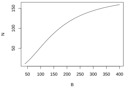
gave the optimal fit (an AIC of 10035). So, given values forB and N we can use the above expression to predict the probability that we will find the opti-mal sequence (in generic problems of this type). Treating the logit-transformed success probability `(B, N) as a function of N for fixed B, we can maximise
`(B, N) with respect to N to find an expression for the optimal N. Differ-entiating `(B, N) with respect to N and setting the derivative equal to zero gives
N = − ˆ
β1
2( ˆβ2+ ˆβ3/B2)
,
50 100 150 200 250 300 350 400
50
100
150
B
[image:12.612.169.422.164.346.2]N
Figure 2: Optimal choice ofN for a given budgetB based on logistic regression analysis of simulation results
by the above expression. Rounding the estimated logistic regression coefficients to 4 decimal places for clarity we have
`(B, N) = logit(E[Y]) = 0.3884 + 0.0199N−0.0001N2−1.3429N2/B2, (2)
and therefore,
N = 0.0199
2(0.0001 + 1.3429/B2). (3)
So, for example, when B = 100 we get N '53 (to the nearest integer) using the unrounded values for the logistic regression coefficients. The estimated relationship between the “optimal”N andB is displayed in Figure 2.
50 100 150 200 250 300 350 400
0.5
0.6
0.7
0.8
0.9
1.0
B
P(optimal in B)
●
●
●
● ●
●
●
[image:13.612.135.456.259.488.2]N chosen optimally N=B/2
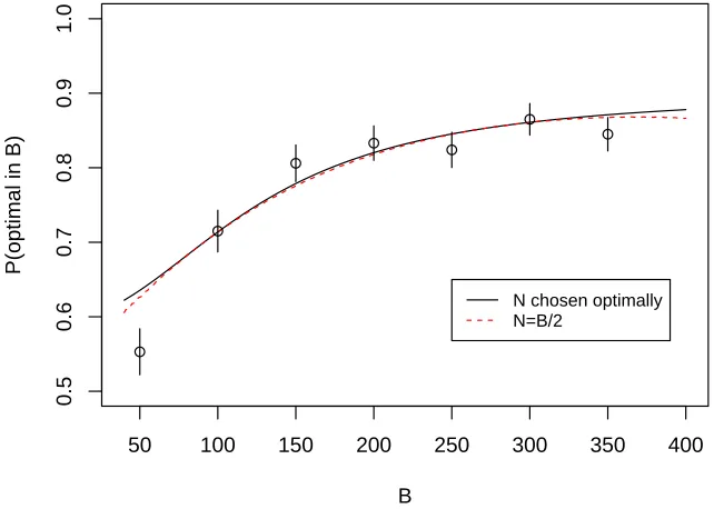
To validate whether the logistic regression model (2) provides a good fit to the simulated data, and hence whether our simple guidance on the choice ofN
will be of practical relevance, we performed a validation simulation study. For each value of B in {50,100,150,200,250,300,350} we generated 1000 “prob-lem scenarios” randomly using the procedure detailed above. For each scenario we performed the usual emulator fitting/evaluation process on a simple ran-dom sample of sequences of sizeN =B/2. We recorded the proportion of the scenarios in which the optimal sequence was found. These empirical propor-tions are unbiased estimates of the true probabilities that the optimal sequence would be found in theB evaluations and are represented by the circles in Fig-ure 3; the vertical lines give approximate 95% confidence intervals for the true probabilities. Our estimates of the probabilities from the independent valida-tion simulavalida-tions match up well with those predicted from our logistic regression model, apart from whenB= 50 where we see that the logistic regression model overestimates the probability slightly. Overall, these simulations would suggest that the logistic regression model is sufficiently accurate at predicting the proba-bility of successfully finding the optimal sequence, over a wide range of plausible scenarios. They also suggest that choosing N =B/2 seems a sensible, simple default option in the absence of other specific information.
7
Cross entropy optimization-based training
sam-ple simulations
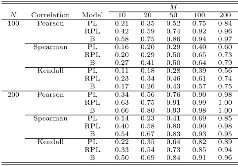
As an alternative to choosing the training sample via a random sample, we have investigated the following simple alternative. For a training sample of size
M
N Correlation Model 10 20 50 100 200
100 Pearson PL 0.21 0.35 0.52 0.75 0.84
RPL 0.42 0.59 0.74 0.92 0.96
B 0.58 0.75 0.86 0.94 0.97
Spearman PL 0.16 0.20 0.29 0.40 0.60
RPL 0.20 0.29 0.50 0.65 0.73
B 0.27 0.41 0.50 0.64 0.79
Kendall PL 0.11 0.18 0.28 0.39 0.56
RPL 0.23 0.34 0.46 0.61 0.74
B 0.17 0.26 0.43 0.57 0.75
200 Pearson PL 0.34 0.56 0.76 0.90 0.98
RPL 0.63 0.75 0.91 0.99 1.00
B 0.66 0.80 0.93 0.98 1.00
Spearman PL 0.14 0.23 0.41 0.69 0.85
RPL 0.40 0.58 0.80 0.90 0.98
B 0.54 0.67 0.83 0.93 0.95
Kendall PL 0.22 0.35 0.64 0.82 0.89
RPL 0.33 0.54 0.73 0.85 0.94
[image:15.612.183.424.287.455.2]B 0.50 0.69 0.84 0.91 0.96