Large substitution boxes with efficient combinational implementations

(1)

Theses

Thesis/Dissertation Collections

8-1-2013

Large substitution boxes with efficient

combinational implementations

Christopher A. Wood

Follow this and additional works at:

http://scholarworks.rit.edu/theses

This Thesis is brought to you for free and open access by the Thesis/Dissertation Collections at RIT Scholar Works. It has been accepted for inclusion in Theses by an authorized administrator of RIT Scholar Works. For more information, please [email protected].

Recommended Citation

(2)

with Efficient Combinational Implementations

by

Christopher A. Wood

A Thesis Submitted in

Partial Fulfillment of the Requirements for the Degree of

Master of Science in

Computer Science

Supervised by

Stanisław Radziszowski

Department of Computer Science

B. Thomas Golisano College of Computing and Information Sciences Rochester Institute of Technology

Rochester, New York

(3)

The thesis “Large Substitution Boxes with Efficient Combinational Implementations” by Christo-pher A. Wood has been examined and approved by the following Examination Committee:

Stanisław Radziszowski Professor

Thesis Committee Chair

Marcin Lukowiak Associate Professor

Alan Kaminsky Professor

(4)

Dedication

(5)

Acknowledgments

This work would not have been possible without the unwavering guidance and support from Staszek and Marcin. Three years have passed since they first introduced me to the wonders of cryptographic and applied security research, and ever since we have shared many meetings, conversations, meals, and coffee breaks that I will always cherish. I am truly grateful to have been given the opportunity to work and study with such extraordinary professors. I am also extremely grateful for the assistance from Alan, whose diligence and extreme attention to detail in everything he does inspires me to improve as a student and researcher. Finally, I would give special thanks to Michael, who has always provided endless encouragement since we started working together. Perhaps one of these days I’ll take his advice and slow down to enjoy other aspects of life.

I would also like to thank David Canright for his very thorough discussions to help me under-stand his S-box constructions, Ren`e Peralta for his kind explanations about his combinational logic minimization techniques, Christof Paar for helpful pointers and his timely advice, and Nele Mentens for her help and example Magma code. These profoundly influential people have shown me the true benefits of collaborative research.

I would also like to thank my friends for their help and support during this work. Greg Knox and Khrystin Matero have spent many years showing me how to balance work and life, and I cannot thank them enough for their continued support and encouragement. I could not ask for better friends. Kaitlin Corbin has also been nothing but supportive, caring, and compassionate during this work. I truly appreciate everything she has done for me. Sam Skalicky has also been a wonderful friend over the past couple of years who helped me a great deal with this research. In addition to his very thorough paper edits and discussions of various hardware-related topics I encountered along the way, he also teared me away from the lab for several much-needed meals and coffee breaks to help keep me sane. I hope I can return the favor as he continues with his PhD. I would also like to thank Ganesh Khedkar for his extensive help with the Synopsys tool and many discussions about gate-level optimizations. I’m very fortunate to have spent the last couple weeks in Rochester working by his side and filling up on mango custard at the Indian food buffet.

I would like to give special thanks to my family, especially my older brother, Robert. As the middle child, I’m fully aware that I can be somewhat bothersome, so I appreciate all the late-night telephone calls and emergency paper edit sessions that we had together. It will be a long time before I can adequately thank him for every sacrifice he made to help me, but it will happen soon enough. Also, I would like to thank my sister, Jessica, who has always been supportive throughout my studies at RIT.

(6)

Abstract

Large Substitution Boxes

with Efficient Combinational Implementations

Christopher A. Wood

Supervising Professor: Stanisław Radziszowski

At a fundamental level, the security of symmetric key cryptosystems ties back to Claude Shannon’s properties of confusion and diffusion. Confusion can be defined as the complexity of the relationship between the secret key and ciphertext, and diffusion can be defined as the degree to which the influence of a single input plaintext bit is spread throughout the resulting ciphertext. In constructions of symmetric key cryptographic primitives, confusion and diffusion are commonly realized with the application of nonlinear and linear operations, respectively. The Substitution-Permutation Network design is one such popular construction adopted by the Advanced Encryption Standard, among other block ciphers, which employs substitution boxes, or S-boxes, for nonlinear behavior. As a result, much research has been devoted to improving the cryptographic strength and implementation efficiency of S-boxes so as to prohibit cryptanalysis attacks that exploit weak constructions and enable fast and area-efficient hardware implementations on a variety of platforms. To date, most published and standardized S-boxes are bijective functions on elements of4or8bits. In this work,

we explore the cryptographic properties and implementations of 8and16 bit S-boxes. We study

the strength of these S-boxes in the context of Boolean functions and investigate area-optimized

combinational hardware implementations. We then present a variety of new8 and16 bit S-boxes

(7)

List of Tables

2.1 Strict Avalanche Criteria (SAC) visualization for the AES S-box. . . 25

3.1 Table of highly nonlinear power mappings with good differential uniformity prop-erties. . . 29

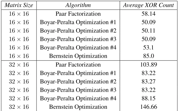
4.1 Comparison of different optimization algorithms for the target16×16and32×16 matrices in this work. The average XOR counts were gathered by populating the entries of matrices with nonzero entries with probabilityp = 0.5over a series of 500trials. . . 42

4.2 Comparison of the factorization time using the sequential and parallel factorization programs. . . 45

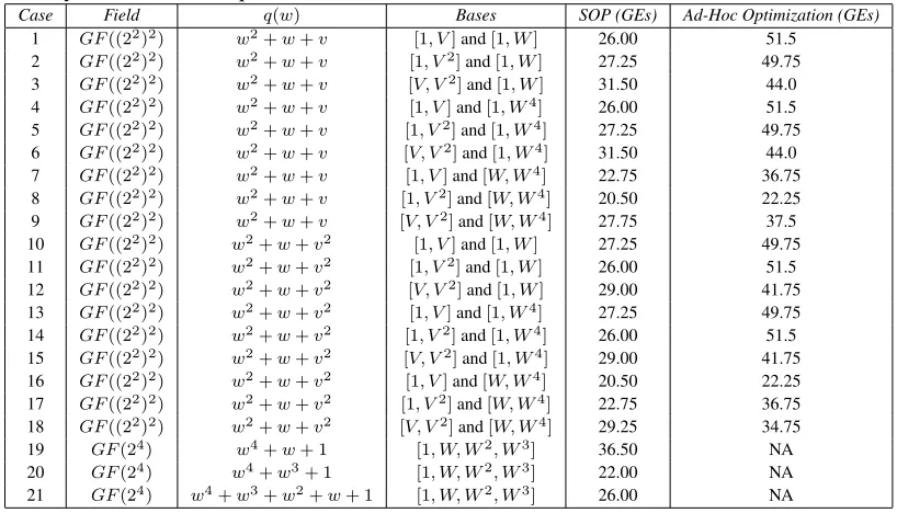
4.3 Hardware area requirements for a variety of inversion circuits for fields isomorphic toGF(24_{). The Sum of Products (SOP) entries are unoptimized circuits derived} directly from the corresponding truth table, and the optimized entries are those min-imized using our modified version of the Boyar-Peralta technique. . . 53

5.1 Required XOR gates forGF(22)arithmetic operations using polynomial and nor-mal bases. Note that each multiplication operation requires three AND gates. . . . 64

5.2 Optimized costs of polynomial scaling inGF((22)2). . . 66

5.3 Optimized costs of polynomial square-scaling inGF((22)2)[13]. . . 67

5.4 Optimized costs of normal scaling inGF((22)2). . . 69

5.5 Optimized costs of normal square-scaling inGF((22)2)[13]. . . 71

5.6 Subfield arithmetic costs ((A)dditions, (M)ultiplications, (Sq)uares, (I)nversions, (SS)quare-scales, (Sc)ales) for finite field arithmetic operations inGF((22)2) us-ing polynomial and normal bases. . . 71 5.7 Total arithmetic operations using the Itoh-Tsujii inversion algorithm for varied

(11)

6.1 AES S-box alternatives with optimized basis change matrices and an un-merged

circuit design. For space, we denote each irreducible polynomials(v), constantc, and binary matrix (A,T, andT−1in row order) as a hexadecimal string. Also note thatΣ,Π, andΛare given in their standard polynomial basis representation. With the basis elements given for all subfields, one may easily convert to the proper basis

representation using the software that produced these results. . . 88

6.2 AES S-box alternatives with optimized basis change matrices and a merged circuit design. For space, we denote each irreducible polynomial s(v), constant c, and binary matrix (A, T, and T−1 in row order) as a hexadecimal string. Also note thatΣ,Π, andΛare given in their standard polynomial basis representation. With the basis elements given for all subfields, one may easily convert to the proper basis representation using the software that produced these results. . . 89

6.3 Precomputed values for the forward of the alternative AES S-box. . . 93

6.4 Precomputed values for the inverse of the alternative AES S-box. . . 94

6.5 Strict Avalanche Criteria (SAC) visualization for the alternative AES S-box. . . 94

6.6 Differential uniformity and nonlinearity of all bijective power mappings overGF(28) defined by the AES irreducible polynomialp(v) =v8+v4+v3+v+ 1. . . 97

6.7 Differential uniformity and nonlinearity of all bijective power mappings overGF(28) defined by the AES irreducible polynomialp(v) =v8+v4+v3+v+ 1. The branch numbers are largely influenced . . . 100

A.1 Irreducible Polynomials forGF(22) . . . 110

A.2 Irreducible Polynomials forGF(24)/GF(22) . . . 110

A.3 Irreducible Polynomials forGF(28)/GF(24)/GF(22) . . . 110

A.4 Irreducible Polynomials forGF(216)/GF(28)/GF(24)/GF(22) . . . 110

B.1 Table #1 of the optimal basis selections and relevant S-box construction information for a separate S-box implementation. . . 115

(12)

B.7 Table #2 of the optimal basis selections and relevant S-box construction information

for a merged S-box implementation. . . 121 B.8 Table #3 of the optimal basis selections and relevant S-box construction information

for a merged S-box implementation. . . 122 B.9 Table #4 of the optimal basis selections and relevant S-box construction information

for a merged S-box implementation. . . 123

(13)

List of Figures

2.1 Visual depiction of the Fast Walsh Transform that is used to calculate the Walsh

spectrum for the Boolean functionf = (10101100). . . 18

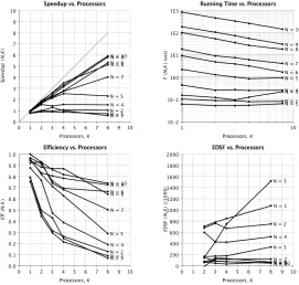
4.1 Speedup metrics for the parallel implementation of Boyar and Peralta’s technique

using tie breaker #1 with16×16matrices. In these graphs we useN = 1to denote

7×7matrices,N = 2to denote8×8matrices, etc. . . 46

4.2 Speedup metrics for the parallel implementation of Boyar and Peralta’s technique

using tie breaker #1 with merged32×16matrices. In these graphs we useN = 11

to denote22×11matrices,N = 2to denote24×12matrices, etc. . . 46

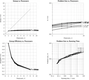
4.3 Sizeup metrics for the parallel implementation of Boyar and Peralta’s technique

using tie breaker #1 with merged16×16 and unmerged matrices. This data was

collected by running tests for matrices of size7×7to16×16matrices. . . 47

4.4 Sizeup metrics for the parallel implementation of Boyar and Peralta’s technique

using tie breaker #1 with merged32×16 and unmerged matrices. This data was

collected by running tests for matrices of size22×11to32×16matrices. . . 47

4.5 RTL schematics for the smallestGF((22)2)andGF(24)inversion circuits gener-ated with the Synopsys tool. . . 54

5.1 All possible tower field representations for GF(216). Our constructions use the

isomorphic fieldGF((((22)2)2)2). . . 56 5.2 Polynomial basis inverter inGF((22)2). . . 57 5.3 Normal basis inverter forGF((22)2). . . 59

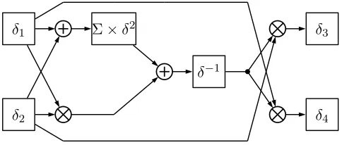
5.4 Polynomial combinational circuit for computing the multiplicative inverse of an

elementδ =γ1v+γ2inGF(22)(i.e.δ−1). . . 60

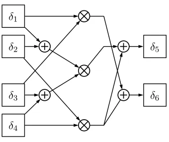
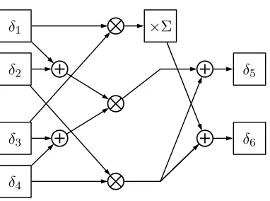
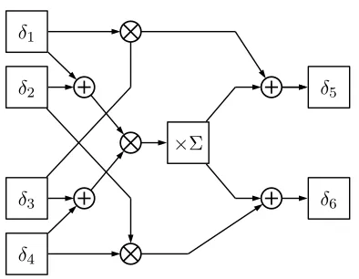
5.5 Polynomial combinational circuit for computing the product ofδ1 =γ1v+γ2and

δ2=γ3v+γ4 inGF(22). . . 61

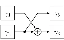
5.6 Polynomial combinational circuit for scaling an elementδ1 =γ1v+γ2by a constant

δ2=γ3vinGF(22). . . 61

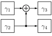
5.7 Polynomial combinational circuit for scaling an elementδ1 =γ1v+γ2by a constant

δ2=γ3v+γ4 inGF(22). . . 62

(14)

5.10 Normal combinational circuit for computing the product of two elements δ1 =

γ1v2+γ2vandδ2 =γ3v2+γ4vinGF(22). . . 63

5.9 Square-scale circuit inGF(22)whenΣ =v+ 1. . . 63

5.11 Polynomial basis multiplier forGF((22)2). . . 65

5.12 Normal basis multiplier forGF((22)2). . . 68

5.13 High-level diagram for a merged S-box circuit. . . 81

(15)

Chapter 1

Introduction

1.1

Motivation

The cryptographic strength of symmetric key cryptosystems is traditionally based on Claude Shan-non’s properties of confusion and diffusion [69]. Confusion can be defined as the complexity of the relationship between the secret key and ciphertext, and diffusion can be defined as the degree to which the influence of a single input plaintext bit is spread throughout the resulting ciphertext. Substitution-permutation networks (SPNs) are natural constructions for symmetric-key cryptosys-tems that realize confusion and diffusion through substitution and permutation operations, respec-tively [72]. In SPN designs for symmetric-key cryptosystems, the substitution step is a nonlinear operation that improves the overall confusion, while the permutation step is a linear operation that increases the measure of diffusion. Formally, an SPN design is defined as follows.

Definition 1. Let l, m, andNr be non-negative integers and SS : {0,1}l _{→ {}₀_,₁_}l _and _SP _:

{1, ..., lm} → {1, ..., lm}be permutations. LetP =C ={0,1}lm_{, and let}_{K ⊆}₍_{₀_,₁_}lm₎Nr+1₎

consist of all possible key schedules that could be derived from an initial key K using the key scheduling algorithm. For a key schedule(K1, ..., KNr+1₎_{, we encrypt the plaintext}_x_using

algo-rithm 1.

Typically, the substitution step (layer), often referred to as the S-box, is theonlynonlinear op-eration in a symmetric-key crpytosystem. As such, it is critically important in the construction of cryptographically strong block ciphers that are resilient to common cryptanalysis attacks, includ-ing linear, differential, and algebraic attacks, among others. Furthermore, as these cryptanalysis efforts have evolved over the past few decades, and with the selection of the Advanced Encryption Standard (AES) as the standard for symmetric-key block ciphers [28], the construction of crypt-graphically “strong” S-boxes with efficient hardware and software implementations has become a topic of critical research.

1.2

Contribution of the Thesis

(16)

Algorithm 1SPN(x, SS, SP,(K1, . . . , KNr+1)) w0 ←x

forr = 1→Nr−1do

ur←wr−1⊕Kr

fori= 1→mdo

vr_<i>←SS(ur_<i>)

end for wr _←₍_vr

SP(1), . . . , v

r SP(lm))

end for

uNr _←_wNr−1_⊕_KNr

fori= 1→mdo

vNr

<i> ←SS(u Nr

<i>) end for

y←vNr⊕K

Nr+1

returny

Combinational implementations of the AES S-box have been well-studied for over a decade [65, 67, 53, 13, 10]. To date, the best known AES S-box from an area perspective requires only

32AND and83XOR/XNOR gates. Following in the spirit of reducing this area requirement even

further, we found an AES S-box candidate that uses the same construction as the one of Canright in [13] but uses a different pair of basis change matrices. If Boyar and Peralta’s logic minimization techniques are applied to this particular representation we may be able to bring the gate count be-low the current record. In addition to studying AES S-box alternatives, we also programmatically explored area-optimized S-boxes overGF(28)defined by all other29possible irreducible polyno-mials. We found another suitable S-box that has even less gates than Canright’s construction prior to logic gate optimizations, which may be of use in other cryptographic algorithms that need an 8-bit S-box. The security properties of this S-box are fully explored using the metrics we identify in Chapter2.

Our work on programmatically finding area-optimized S-boxes was then scaled up toGF(216).

For the21 smallest degree 16 irreducible polynomials overGF(2), we found several S-box

con-structions from the set of all candidate concon-structions that have minimized area footprints without combinational logic optimizations. We were not able to analyze the security properties of these S-boxes due to the complexity of computing each metric, though we expect that its similarity to the AES S-box leads to very similar, and appropriately stronger security properties due to the increased bit size.

It is uncertain whether or not the 16-bit S-boxes will ever be used or needed. Nevertheless, the security and implementation aspects of such S-boxes may reveal new avenues of research that can be further explored in the context of smaller S-boxes. For example, combinational logic minimization

techniques such as factoring are much more computationally intensive for16×16 matrices over

GF(2) than 8×8 matrices. As a result, we explored parallel implementations of minimization

(17)

A more tangible contribution of this work is the development of software tools for the following tasks:

1. Composite Galois field arithmetic (Python)

This software is capable of performing arithmetic inGF(p),GF(pn), andGF((pn)m). It is useful for learning the fundamentals of Galois fields and simple composite fields.

2. Optimized linear and nonlinear circuit minimization (Java)

This suite of programs are capable of optimizing linear and nonlinear circuits using the com-binational minimization techniques discussed in Chapter 4. We use these programs to re-duce the overall area requirements for our candidate S-box constructions and analyze the area footprint of inversion circuits for the fieldsGF(24)andGF((22)2). The linear circuit opti-mizations come with sequential and parallel implementations that enable larger circuits to be processed in less time.

3. Cryptographic mapping security analysis (Python)

This compact program implements all of the metric computations discussed in Chapter 2. It does not rely on any external libraries outside of the core Python libraries for all of its

implementations. It supports a complete workflow for analyzing any arbitrary mappingF :

GF(2n)→GF(2n).

4. S-box construction and combinational area counting (Magma)

This suite of programs was leveraged to programatically derive area-optimized combinational circuits for all candidate 8 and 16-bit S-boxes. One may use these programs to determine minimized gate counts for many Galois field arithmetic operators, including addition, multi-plication, squaring, scaling (multiplication by a constant), and inversion. In addition, one may use these programs to search for suitable affine transformations used to construct S-boxes.

We describe each of these software deliverables in their respective chapters of this work. As we note in the conclusion, future work will entail continued development of these tools for crypto-graphic research. In particular, we plan on including normal basis arithmetic in the Galois field library, developing advanced circuit minimization techniques (e.g. SAT solver reductions [34]), and integrating our security analysis code into the SAGE software package [71].

(18)

ASICs. With this preliminary work, we then discuss the methodology in which we count the number of required gates to implement a particular S-box construction based on the Galois field multiplica-tive inverse in Chapter 5. Our results consist of an extension of Canright’s [13] optimizations using mixed basis representations of Galois field elements. We then conclude in Chapters 6 and 7 with a presentation of our proposed 8-bit AES alternative S-boxes and 16-bit S-box constructions, as well as a discussion of future work.

1.3

Mathematical Foundations

Galois Fields, commonly referred to as finite fields, and Boolean functions play a critical role in the design, development, and analysis of a variety of cryptographic primitives. Galois fields are commonly used to define efficiently computable cryptographic functions, such as the S-box in SPN designs, whereas Boolean functions typically serve as tools for measuring the strength and resilience of cryptographic operations to common cryptanalysis attacks. In this section we provide an intro-duction to these mathematical constructs as a foundation for the rest of the thesis.

1.3.1 Galois Fields

Much of number-theoretical cryptography is founded upon the mathematical structures of groups, rings, and fields. For completeness, we define these structures and their relevant properties below. The reader may find a more rigorous treatment in [48].

Definition 2. Anabelian grouphG,+iconsists of a setGand an operation+defined on its elements

that satisfies the following properties:

• Gis closed under+(for alla, b∈Git is true thata+b∈G)

• Associativity holds with respect to the+operator (for alla, b, c∈Git is true that(a+b)+c=

a+ (b+c))

• Commutativity holds with respect to the+operator (for alla, b∈ Git is true thata+b =

b+a)

• There exists an identity element0∈Gsuch that for alla∈Git is true thata+ 0 =a

• For all elementsa∈Gthere exists a corresponding inverse elementb∈Gsuch thata+b= 0 A very common example of a group ish_Z,+i, that is, the set of integers with respect to the addition operator.

Definition 3. A ring hR,+,·i consists of a set R with two binary operations+,· defined on its

(19)

• The two operations+and·are related by thelaw of distributivity. That is, for alla, b, c∈R

it is true that(a+b)·c= (a·c) + (b·c).

Again, a common example of a ring is h_Z,+,·i, that is, the set of integers with the binary addition and multiplication operators.

Definition 4. A structurehF,+,·iis afieldif the following two conditions are satisfied:

• hF,+,·iis a commutative ring.

• For all elements of_F, there is an inverse element in_Fwith respect to·, except for the element

0, the neutral (identity) element ofh_F,+i.

More specifically, a structureh_F,+,·iis a field if and only if bothh_F,+iandh_F\ {0},·iare abelian groups and the law of distributivity applies. If the set of elements inFis finite, thenFis a

Galois field. Such fields are commonly denoted asGF(p), wherepis prime.

The set of polynomials over a fieldFis defined asF[x]/p(x), wherep(x)is some irreducible

polynomial overF. IfFis finite withpelements, makingFa cyclic field, thenGF(pn)defines the

set of polynomials overGF(p)modulo an irreducible polynomialp(x)of degreen. For complete-ness, polynomial irreducibility is defined as follows.

Definition 5. A polynomialp(x)isirreducibleover the field_Fif and only if there does not exist two

polynomials q(x) andr(x) with coefficients inFsuch that p(x) = q(x)×r(x), where q(x) and r(x)are of degree>0.

It is well known that for every cyclic Galois fieldGF(pn)there exists at least one elementα

such that every element in the field, with the exception of the neutral element, can be computed asαi for some0 ≤ i ≤ 2p−1. In this case,αis said to be a primitive element, or agenerator, ofGF(pn). With the notion of a primitive element, we now introduce the concept of a primitive polynomial.

Definition 6. A polynomialp(x) of degreenisprimitive over the fieldGF(p)if and only if it is

irreducible overGF(p)and the elementxis a primitive element ofGF(pn).

Another important property to note is the characteristic of a Galois fieldGF(p), which is the smallest positive integerksuch thata+a+· · ·+a

| {z }

ktimes

= 0anda ∈ GF(p). In this work we focus

primarily on fields with characteristic2, often referred to as binary Galois fields. It is also useful to note the concept of a trace, given in the following definition.

Definition 7. Thetraceof an elementα∈GF(pn₎_{relative to the subfield}_GF₍_p₎_{is defined as}

T r_GF₍_pn₎_/GF₍_p₎(α) =α+αp+αp 2

+· · ·+αpn−1.

In this case, the set{α, αp, αp2, . . . , αpn−1}is the set of conjugates ofα.

Finally, the cyclotomic cosetCsmodulo2n−1[50] is defined as

Cs={s, s·2,· · ·,2·2ns−1},

wherensis the smallest positive integer such thats≡s2ns−1 mod 2n−1. Also,sis denoted as

the coset leader of the cyclotomic cosetCs. Computations of these sets deal with elements in the

(20)

1.3.2 Bases of Galois Fields

It is natural to represent an element in the fieldGF(pn₎_{as a standard polynomial of the form}

p(x) =an−1xn−1+an−2xn−2+...+a2x2+a1x+a0,

whereai ∈GF(p)are the coefficients of the polynomial.

However, when a more rigorous treatment of Galois field bases is needed, GF(pn) may be

viewed as ann-dimensional vector space overGF(p). As a vector space, we see that a basis must exist for the field. For cryptographic applications, the standard (polynomial), normal, and dual basis representations are important elements of study, though in this work we restrict ourselves to only

polynomial and normal bases. With astandard orpolynomial basisfor elements in GF(pn), the

basis elements are represented as successive powers of a primitive element of the field, denotedθi

for0 ≤ i < n. That is, the basisβ may be viewed as[θ0, θi, . . . , θn−1]. As a proper basis, every elementα in the field may be represented as a linear combination of the elements in the basis as follows:

α =an−1θn−1+an−2θn−2+· · ·+a1θ+a0,

whereai ∈GF(p)for all0≤i < n.

With anormal basisrepresentation for elements inGF(pn), the basis elements are defined as

θqi for 0 ≤ i < n, whereθis a primitive element of the field and all basis elements are linearly independent. In this case, the basisβ may be viewed as[θp0_{, θ}p1_{, . . . , θ}pn−1_{]. With this basis, each}

elementαin the field may be represented as a linear combination of its elements, as shown below,

α =an−1θp

n−1

+an−2θp

n−2

+· · ·+a_p1θp+a₀θ,

whereai ∈GF(p)for all0≤i < n.

1.3.3 Composite Fields

LetGF(2k)be defined by the degreekirreducible polynomialr(z). We may define a polynomial basis for this field as a set ofklinearly independent elements as follows:

B1= [1, α, α2, ..., αk−1],

whereαis a primitive element inGF(2k). With this basis we may write any elementA1_i ∈GF(2k)

as Ai = Pk−1

j=0ajαj, where aj is the coefficient for the αj term and aj ∈ GF(2). With this

representation, the field arithmetic operations of addition, subtraction, multiplication, and inversion are defined with respect toB1 and the subfield GF(2)[1]. In this sense, we say that GF(2k)is

a degree k extension of GF(2), which means that polynomial coefficient arithmetic of GF(2k)

is performed over the subfield GF(2). However, we may refine these arithmetic operations by

choosing a different basis or by using a different construction method for the field. Recent research has focused on the latter using composite fields [65, 67, 53, 13, 9].

Letk = nm, wheren, m ∈ _Z. With this constraint, it is possible to defineGF(2k), which is uniquely represented by the irreducible polynomialr(z), as a degreemextension ofGF(2n_{). Any}

(21)

functional composition of more than one extension field, where one of the fields in this composition is an extension of GF(2)). We denote this composite field as GF((2n₎m_{), where}_GF₍₂n₎_{is the}

ground fieldover which the composite field is defined.

More specifically, acomposite fieldis a pair{GF(2n), p(x) =xn+Pn−1

i=0 pixi, pi ∈GF(2)}

and {GF((2n)m), q(y) = ym +Pm−1

i=0 qiyi, qi ∈ GF(2n)} whereGF(2n) is constructed from GF(2)byp(x), andGF((2n)m)is constructed fromGF(2n)byq(y). We state thatGF((2n)m)

is a degree m extension of GF(2n). This form of extension means that the coefficients of the

polynomials inGF((2n)m)are themselves elements ofGF(2n), and thus all coefficient arithmetic is performed inGF(2n).

Now, we represent elements inGF((2n)m)using a new polynomial basisB2as follows:

B2 = [1, β, β2, ..., βm−1]

Note that now we have m linearly independent elements as opposed to k. Also, β is the root of

a primitive irreducible polynomial of degreem whose coefficients are in the base fieldGF(2n). With this basis we may now represent an elementA0_i ∈GF((2n)m)asA0_i =Pm−1

j=0 a0jβj, where a0_j ∈GF(2n₎_for₀_≤_{j < m}_.

1.3.4 Boolean Functions

A Boolean functions is a functionf :Fn2 → F2. For convenience, letΩnbe the set of all Boolean

functions onnvariables, where|Ωn|= 22

n

. For all Boolean functionsf ∈Ωnthere exists a unique

truth table (TT) or Algebraic Normal Form (ANF) representation [27]. The TT for a Boolean functionf is simply the vector(f(¯0), . . . , f(¯1))), where each element corresponds to an element inF2 ∼=GF(2). The distance between two Boolean functionsf, g ∈Ωnis simply the number of

elements in the TT representation offthat need to change to makef =g. This can easily computed by the Hamming distance between the respective truth tables forf andg.

Alternatively, we may represent Boolean functions in their ANF format as polynomials with coefficients in F2. The process of translating a Boolean functionf to its ANF representation is

called the the algebraic normal transform, and is defined as follows:

f(x0, . . . , xn−1) =

M

(a0,...,an−1)∈Fn2

h(a0, . . . , an−1)xa00x

a1

1 . . . x

an−1

n−1 ,

wherehis a Boolean function.

We denote the Hamming weight of a vector(x0, . . . xn−1) = ¯x ∈ Fn2 as HW(¯x). We denote

the dot product of two vectors x,¯ y¯ ∈ Fn2 as x¯⊕y¯, and is defined as the scalar value x1y1 ⊕

x2y2 ⊕ · · · ⊕xnyn. The inner product of two vectors x,¯ y¯ ∈ Fn2, defined as the vector z¯ =

(x1y1, x2y2, . . . , xnyn), is denoted asx¯·y¯[27].

If we consider the ANF representation of a Boolean function as a nonzero polynomial function

f :F2n →_F₂, then we may representf as a sum of the trace functions over_F₂as follows [36]:

f(x) = X

k∈γ(n)

T rnk

1 (Akxk) +A2n₋₁x2 n₋₁

(22)

whereAk ∈F2nk,A2n₋₁ ∈_F₂,γ(n)is set of all coset leaders modulo2n−1, andn_k is the size of the coset Ck. Iff(x)is a balanced Boolean function, meaning that|{x : f(x) = 1}| = |{x : f(x) = 0}|= 2n−1, then 1.1 reduces to

f(x) = X

k∈γ(n)

T rnk

1 (Akxk). (1.2)

The Walsh and Discrete Fourier transforms are also immensely useful in the mathematical study of Boolean functions. In fact, Boolean functionsf onFn2 can be uniquely identified by theirWalsh transform, where the Walsh transformWf off is an integer-valued function defined for allw¯∈Fn2

as

Wf( ¯w) =

X

¯

x∈_Fn 2

(−1)f(¯x)⊕x¯·w¯

= 2n−2×HW(f(¯x)⊕x¯·w¯).

Informally, the Walsh transform of a given vectorw¯is the difference between the number of input vectorsx¯for whichf(¯x) = ¯w·x¯and the number of input vectorsx¯for whichf(¯x)6= ¯w·x¯. Thus, in a sense, we may interpret the Walsh transform of a particular Boolean function as the collective similarity betweenf(¯x)and the linear functionw¯·x¯.

It is well known thatF2n is isomorphic to_Fn₂, so we may represent an elementα ∈_F₂n as an

n-dimensional vectorw¯overF2. With this observation, we may then seek to measure the similarity

off(¯x)to all linear functionsw¯·x¯by applying the Walsh transform to each possible input vector ¯

wi,0 ≤ i <2n. The result of this procedure is theWalsh spectrum, which simply corresponds to the vector[Wf(α0 ∼= ¯w0), Wf(α1 ∼= ¯w1), . . . , Wf(α2n₋₁∼= ¯w₂n₋₁)].

1.3.5 S-Boxes as(n, m)Boolean Functions

S-boxes are traditionally defined as functionsS :GF(2n)→GF(2m), wheren=m. In the case of Rijndael,n=m= 8. In order to study such S-boxes using one-dimensional Boolean functions, it is necessary to extend the definitions and representations of Boolean functions to multiple dimensions. To do this, we define a vectorial Boolean function F : GF(2n) → GF(2m) (e.g. an(n, m)

S-box) using a vector of m component Boolean functions [17]. More specifically, we letF(x) =

(f1(x), . . . , fm(x)), wherefi : GF(2n) → GF(2)for all 1 ≤ i ≤ m. S-boxes can therefore be

(23)

Chapter 2

Cryptographic Aspects of the Substitution Layer

2.1

Cryptanalysis Attacks

The substitution layer plays a critical role in the security of block ciphers designed with a substi-tution layer for nonlinearity. Over the past several decades, many forms of cryptanalysis attacks have been devised, implemented, and tested on full-size and “toy” versions of block ciphers. In this section, we describe some effective attacks that exploit specific properties of the S-box during the attack. Such attacks have already been studied by Kaminsky et al. [44] in the context of the AES, who cover this topic in more breadth with additional information about side channel attacks, for example. We refer the reader to their survey for more information on recent AES-specific crypt-analysis results. In this work, we use the following attacks as motivation for measuring the strength of S-boxes, which can be perceived as their relative resistance to these attacks. As we will show in Chapter 3, these metrics are then used when designing cryptographically strong S-boxes. We stress that this list of attacks is by no means exhaustive; it simply contains some of the most important published attacks. For the purposes of this work, we chose to focus on this particular subset as they are, in a sense, the most known.

2.1.1 Linear Cryptanalysis

Since S-boxes are typically the only source of nonlinearity and, consequently, confusion, in an SPN design, it is critically important to understand the degree to which they can be approximated as linear equations [72]. For the purposes of this section, we consider only bijective S-boxesS :

{0,1}n _{→ {}₀_,₁_}n_{. In the context of linear cryptanalysis, we say that for each input element of the}

S-box, which may be viewed as ann-dimensional vector of coordinates(x0, x1, . . . , xn−1), there

is a corresponding set of n independent random variables Xi, 0 ≤ i < n. Similarly, for each

output element of the S-boxy¯ = (y0, y1, . . . , yn−1), there aren corresponding random variables Yi,0 ≤i < n. However, these variables are not specifically independent from each other or from

theXivariables, since the probability of the output depends on the input.

The underlying goal of linear cryptanalysis is to find and exploit some linear combinationXi,1⊕

(24)

deviation, or bias, from the relationship can be exploited in a linear cryptanalysis attack. With this goal as motivation, we begin our discussion of linear cryptanalysis with some more formal definitions.

Definition 8. Letpibe the probability thatPr[Xi= 0]. We define thebiasofxi, denotedi, as the

quantity:

i =pi−1

2.

Now, we consider all possible2n _{random variable combinations for}_n_{variables. For an S-box}

with a 4-bit domain and range, we have a total of8random variables to examine, which, together,

correspond to the 4 input and 4 output bits. Therefore, there are 28 possible combinations that

can be used to calculate biases. Let the n-dimensional vectors a = (a1, a2, . . . , an) and b =

(b1, b2, . . . , bn), where ai, bi ∈ {0,1} for all 1 ≤ i ≤ n correspond to these input and output

elements for the S-box. We can represent all28linear combinations as follows

n

M

i=i aiXi

!

⊕

n

M

i=i biYi

!

= 0,

or, equivalently,

n

M

i=i aiXi

!

=

n

M

i=i biYi

!

.

Using the Piling-Up Lemma presented by Matsui [51], we have

P r[Xi⊕ · · · ⊕Xn= 0] = 1 2 + 2

n−1

n

Y

i=1

i,

which means that

1,2,...,n = 2n−1 n

Y

i=1

i,

where1,2,...,nis the bias ofXi⊕· · ·⊕Xn. This leads to the fundamentally simple (albeit very clever) counting-based attack that is linear cryptanalysis. More specifically, if we use a counting-based method for determining the bias for all possible linear combinations of input and output variables

XiandYj, we can identify input and output variables that are suitable candidates for conducting

a linear cryptanalysis attack. Treating the a andb vectors as binary numbersa and b, we may

tabulate NL(a, b), the number of tuples(x1, x2, ..., xn, y1, y2, ..., yn) such that (y1, y2, ..., yn) = SS(x1, x2, ..., xn)and

n

M

i=i aixi

!

⊕

n

M

i=i biyi

!

= 0.

With the NL(a, b) table, we then compute the bias 1,2,...,n by (NL(a, b)−2n−1)/2n, and from

this, the probability pi that the linear combination Xi ⊕ · · · ⊕Xn = 0 was satisfied, i.e. pi =

(25)

Algorithm 2General Linear Cryptanalysis Attack

Require: P,K,Bx,By,S−1_,_l_,_m

1: Count[K]←[0...2lm]

2: for eachK∈ Kdo

3: Count[K]←0

4: end for

5: for each(x, y)∈ Pdo

6: forK ∈ Kdo

7: V ←[]

8: fori= 1to|By|do

9: v← S−1₍_K_⊕_y

By[i])

10: V =Append(V, v)

11: end for

12: z←L|Bx|

i=1xBx[i]

L|By|

i=1V[i] 13: ifz= 0then

14: Count[K]←Count[K] + 1

15: end if

16: end for

17: end for

18: max← −1 19: K∗ ={0}lm

20: for eachK∈ Kdo

21: ifCount[K]> maxthen

22: max←Count[K]

23: K∗ ←(K)

24: end if

25: end for

26: returnK∗

Using the example linear cryptanalysis attack presented in [72], we give a generalized procedure for realizing this type of attack in Algorithm 2. We borrow the same notation from Stinson in which plaintext elementsxand ciphertext elementsyare bit strings of lengthlm, which can be viewed as the concatenation oflseparatem-bit strings. With this notation, we refer to theith block of length

m in a plaintext (ciphertext) element x (y) asxi (yi),0 ≤ i < l. In our procedure we use P to denote the set of all plaintext and ciphertext pairs collected prior to evaluation, andB_xandB_y are sets of block (random variable) indexes that are used in the predetermined linear combination of S-box input and output elements, respectively. That is, the indexes in Bx andBy correspond to a

selection of random variables corresponding to a linear combination of input and output bits that is satisfied with relatively high or low probability, as determined from theNL(a, b)table. Finally,

we denote the inverse S-box asS−1and the set of all possible candidate keys asK, where for each

(26)

As previously stated, the goal of linear cryptanalysis is to find a set of linear approximations of active S-boxes that help approximate an entire SPN algorithm throughout all of the rounds (with the exception of the last). Matsui [51] showed that the complexity of this known-plaintext attack (i.e. the number of plaintexts required for a successful attack) is proportional to −2, whereis the bias from 1/2 that a linear expression exhibited for the entire SPN-like block cipher. It is generally known that larger S-box biases correspond to larger biases for every round of the block cipher, which is expected since they are typically the only nonlinear components of the algorithm. Therefore, studying the resiliency of S-boxes to this type of attack is critically important in the design of cryptographically strong S-boxes. In Section 2.2 we will discuss the properties of S-boxes in SPN designs that improve the algorithm’s resiliency to this type of attack.

2.1.2 Differential Cryptanalysis

Differential cryptanalysis, first introduced as an attack on the Data Encryption Standard [4], is a chosen plaintext attack that attempts to find and exploit certain occurrences of input and output differences in the last round of a cipher that occur with a high probability [72]. Put another way, for an ideally randomizing block cipher with a sufficiently strong S-box, the probability that a certain output difference∆Y =Yi⊕Yj will occur given an input difference∆X = Xi ⊕Xj is exactly

1/2n_(where_n_{denotes the number of bits in the input}_X_{). For future reference, the pair}_(∆_X,_∆_Y₎

is referred to as a differential. Thus, by finding output differences that occur with high probability for each round of a target cipher, one can establish a relationship between the plaintext and input to the last round of the cipher. Such a relationship is loosely referred to as adifferential trail[29]. Then, by sampling a large number of plaintext and ciphertext pairs, the attacker can guess the key by counting the number of times a given differential trail holds for a candidate key. In ciphers where the round key schedule is invertible, this enables the attacker to uncover the secret key. Clearly, the nonlinearity of the S-box plays a pivotal role in the establishment of the differential characteristic for the entire cipher. Also note that in SPN designs, the key does not influence the coordinates of a differential. For example, given the differential(∆X,∆Y), we have the following:

∆Y =Yi⊕Yj

= (Xi⊕K)⊕(Xj⊕K)

=Xi⊕Xj⊕K⊕K

=Xi⊕Xj

= ∆X

To carry out this attack, the attacker must collect a large sample of plaintext and corresponding ciphertext pairs(X, Y). Given that the S-box is the key to preventing this attack, the attacker then computes a difference distribution tableND, where

ND(∆X,∆Y) =|{(Xi, Xj)∈∆X :S(Xi)⊕S(Xj) = ∆Y}|.

One may observe that in an ideal S-box,ND(∆X,∆Y) = 1for all∆Xand∆Y. However, this is

not possible with bijective S-boxes becauseND(∆X,∆Y = ∆X) = 2n.

We denote thepropagation ratio RD(∆X,∆Y) = ND(∆X,∆Y)/2n, which may be

(27)

propagation ratio, and further assume that∆Y is equal to∆X0in a differential(∆X0,∆Y0)with a high propagation ratio in roundr+ 1. We may then combine these differentials together, forming a subset of the previously mentioned differential trail, and compute the resulting propagation ratio as

RD(∆X,∆Y)·RD(∆X0,∆Y0). By continuing this process, we may obtain the propagation ratio

for a differential trail of the allNr−1rounds of the block cipher (up to the last round). The attacker

can then use this differential trail to determine which candidate keys satisfy the input and output difference with the highest probability. A generic description of this process is given in Algorithm 3. Note that we now require a new parameterB_tthat contains the indexes that of the output elements

y andy0 such thatyi = y_i0 for alli ∈ Bt. Counting keys that do not satisfy this constraint would

introduce random noise into the attack, and should thus be avoided.

2.1.3 XL and XLS Algebraic Attacks

Thanks to Courtois et al. [21], we know that it is possible to represent block ciphers as overdefined systems of multivariate quadratic (MQ) equationsA, where each equationlk ∈Ais of the form

lk =

X

i,j

ai,j,kxixk+

X

i

bi,kxi+ck= 0,

and ai,j,k, bi,k, ck ∈ GF(2). Solving such a system is known to be an NP-hard [33] problem.

However, solving a system of linear equations can be done in polynomial time using techniques such as Gaussian elimination. In 2000, Shamir, Courtois, Klimov, and Patarin [21] introduced a

technique known as eXtended Linearization (XL), which transforms a MQ problem ofmequations

and n variables into a (much) larger system of solvable linear equations. This technique is an

extension of the “linearization” technique first introduced in [46].

The procedure works by first generating a set ofD−2(D ≥ n/√m) new variables with all

powers less than or equal to D−2. Referring to the example given in [47], if we have a set of

variables{x, y, z}withD= 4, then the resulting set of variables is{x, y, z, x2, y2, z2, xy, xz, yz}. Each variable in this set is then multiplied by the original mequations. Then, for each resulting equation, the individual monomial terms are all replaced by a distinct new variables. For example,

for an equationli =x3yz+xy = 0, we would generate a corresponding equationli =a+b= 0,

wherea=x3yzandb=xy, respectively. From here, we have a set of linear equations that can be solved in polynomial time. Of course, the complexity of this process depends greatly on the

selec-tion ofDand the originalnandmparameters in the MQ system. Since the algebraic expression

of SPN ciphers has a direct impact on the form of the MQ system, it is clear that improving the complexity of this expression helps thwart the success of this attack. A formal description of the XL algorithm is shown in Algorithm 4.

To date, the XL attack has failed to break popular ciphers such as Rijndael and Serpent. How-ever, Courtois and Pieprzyk [22] discovered a way to modify the XL attack to account for the sparse set of equations that are introduced in the process. This variation, coined as the eXtended Sparse Linearization (XSL) attack, is different in that the process by which new variables are defined and

then subsequently multiplied by themequations in the MQ system is modified to only work with a

(28)

Algorithm 3General Differential Cryptanalysis Attack

Require: P,K,Bx,By,Bt,S−1_{, l, m}

1: for eachK∈ Kdo

2: Count[K]←0

3: end for

4: for each(x, y, x0, y0)∈ Pdo

5: R←T rue

6: fori= 1to|B_t|do

7: ifyBt[i]6=y 0

Bt[i]then

8: R←F alse

9: end if

10: end for

11: ifR=T ruethen

13: D←[]

14: fori= 1to|By|do

15: v← S−1₍_K_⊕_y

By[i])

16: v0 ← S−1₍_K_⊕_y0 By[i])

17: D←Append(D, v⊕v0)

18: end for

19: match←1

20: fori= 1to|B_y|do

21: match←match∧(D[i] = ∆Y∗)

22: end for

23: ifmatch= 1then

24: Count[K]←Count[K] + 1

25: end if

26: end for

27: end if

28: end for

29: max← −1

30: K∗ ← {0}lm

32: ifCount[K]> maxthen

33: max←Count[K]

34: K∗ ←(K)

35: end if

36: end for

(29)

Algorithm 4Extended Linearization

Require: F, m, n, A={l1, . . . , lr}

1: Generate all polynomial equationsl0_i =

Qk

i,jxi,j

li, wherek≤D−2.

2: varM ap={} 3: forl0_i=l₁0 tol_k0 do

4: forj = 1to|l_i0|do .For each term inl_i0

5: ifpj 6∈varM apthen

6: v=|varM ap|+ 1 .Generate a new variable not in the map

7: varM ap[v] =l0_i[j]

8: end if

9: l_i0[j] =varM ap[l0_i[j]] .Perform substitution

10: end for

11: end for

12: Perform Gaussian elimination for the modified system of equations{l₁0, . . . , l0_r}.

13: whileThere exists at least one univariate equationl0_iin the powers ofxido

14: Solvel0_iover the fieldF

15: Simplify the set of equations{l0₁, . . . , l_r0}

16: end while

17: Perform backwards substitution to find the original variables

implication of this attack is that it does not grow with the number of rounds in the cipher, as is the case with the traditional linear and differential cryptanalysis attacks. Rather, the complexity is based solely on the structure of the cipher, and more specifically, on the complexity and degree of the S-box algebraic expression.

2.1.4 Interpolation Attacks

Interpolation attacks consider the problem of representing a cipher as a high-order polynomial with key-dependent coefficients [42]. The intuition behind this representation is that by then solving for these coefficients it is possible to deduce the secret key. Given a fieldGF(2k_{), such a polynomial} p(x)is obtained using Lagrangian interpolation. In particular, withn= 2k distinct input elements

x1, . . . , xkand output elementsy1, . . . , yk, we may determine a polynomialp(x)by

p(x) =

n

X

i=1

yi

Y

1≤j≤n,j6=i

x−xj xi−xj.

(30)

Theorem 1. [42] Given an iterated block cipher of block sizel, it is possible to express the ouput from roundNr−1as a polynomial of the plaintext withmcoefficients. Withbkey bits in the last

round, there exists an interpolation attack of time complexityO(2b−1(l+ 1)) that requiresl+ 1

known plaintexts which can successfully deduce the secret key.

In the case of Rijndael, the polynomial used to represent the S-box is:

p(x) = 05x254+ 09x253+F9x251+ 25x247+F4x239+ 01x223+B5x191+ 8F x127+ 63,

where all coefficients are hexadecimal numbers, and thus elements of the fieldGF(28). This al-gebraic expression was obtained using Lagrangian interpolation [29] (this technique is discussed in more detail in Chapter 3). Since the degree ofp(x)is9, and so this class of interpolation attack is not feasible. However, the algebraic simplicity of Rijndael’s S-box, which is directly correlated to the complexity of the polynomial representation for the entire cipher, leaves many cryptographers skeptical about its security and future susceptibility to related attacks.

2.2

Efficient Computations of Cryptographic Properties of S-Boxes

The strength of S-boxes can be measured in the context of Galois fields and Boolean functions. In this section, we focus on several important measurements of the cryptographic strength of S-boxes. We then present security metrics that can be used in the context of Boolean functions, such as nonlinearity, resiliency, the strict avalanche criterion, and algebraic immunity. We also present source code that may be used to efficiently compute such metrics.

2.2.1 Linear Approximation and Difference Distribution

With the advent of linear and differential cryptanalysis on SPN block ciphers, the contents of the linear approximation and difference distribution tables, which are highly dependent on the S-box used in such block ciphers, are critical in determining a particular construction’s susceptibility to these attacks. Based on the definitions given in the preceding section, we can compute theNL(a, b)

matrix using the procedure outlined in Algorithm 5. The exhaustive nature of this algorithm yields a time complexity ofO(24n). As such, whenn≈ 16, computing this table cannot be done easily on a normal computer. An ideal S-box will have probabilities around 0.5 for all input and output combinations, meaning that linear combinations do not occur with non-random frequency, which is needed to carry out a successful linear cryptanalysis attack.

As discussed in the previous section, differential cryptanalysis relies on the difference distribu-tion table, ND(∆X,∆Y). Since this table is generated from an exhaustive check of all input and

output differences, we compute it very similar toNL(a, b) using Algorithm 6. However, we now

only have a time complexity ofO(22n).

2.2.2 Nonlinearity

(31)

Algorithm 5NL(S, n)

1: NL←zeros(1...2n−1,1...2n−1)

2: fora= 0to2n₋₁_do

3: forb= 0to2n−1do

4: forx= 0to2n−1do

5: fory = 0to2n₋₁_do

6: ifS(x) =yand HW((x∧a)⊕(y∧b)) = 0then

7: NL(a, b)←NL(a, b) + 1

8: end if

9: end for

10: end for

11: end for

12: end for

Algorithm 6ND(S, n)

1: ND ←zeros(1...2n−1,1...2n−1)

2: forx1 = 0to2n−1do 3: forx2= 0to2n−1do 4: ∆X=x1⊕x2 5: ∆Y =S(x1)⊕S(x2)

6: ND[∆X,∆Y]←ND[∆X,∆Y] + 1

7: end for

8: end for

9: returnND

which means that there will be less input and output sums for the S-box with high magnitude biases. This will typically lead to more evenly distributed entries in the NL(a, b) table that are close to

2n−1, which yield biases of0.

For a Boolean functionf, the nonlinearityN_lis defined as the minimum distance betweenfand all possible affine functions onnvariables. Formally, we define the nonlinearity as follows [27]:

N_l(f) = min

φ∈Ωn

d(f, φ),

where d(f, g) =HW(f ⊕g) (i.e. the Hamming distance between two functions f and g). The

maximum value forNlis2n−1−2n/2−1. It is also convenient to use the Walsh-Hadamard transform

of a Boolean functionf asWf(u) =

P

x∈_Fn

2(−1)

f(x)⊕(u·x)_{, where}_w _∈

Fn2 andw·xis the inner

product of the two vectorsw, x∈_F₂[27], to define the nonlinearity of a functionf as

N_l(f) = 2n−1−1

2maxu∈Fn2

|Wf(u)|. (2.1)

(32)

1

0

1

0

1

0

1 + 1 = 2

0 + 1 = 1

1 + 0 = 1

0 + 0 = 0

−1 + 1 = 0

−1 + 0 =−1

−0 + 1 = 1

−0 + 0 = 0

2 + 1 = 3

1 + 0 = 1

−1 + 2 = 1

−0 + 1 = 1

0 + 1 = 1

−1 + 0 =−1

−0 +−1 =−1

3 + 1 = 4

−1 + 3 = 2

1 + 1 = 2

−1 + 1 = 0

1 +−1 = 0

−(−1) + 1 = 2

−1 +−1 =−2

−(−1) +−1 = 0

Figure 2.1: Visual depiction of the Fast Walsh Transform that is used to calculate the Walsh

spec-trum for the Boolean functionf = (10101100).

nonlinearity for such functions is 2n−1 −2n/2, and we call a functionF maximally nonlinear if it reaches this bound [31]. Maximally nonlinear Boolean functions are also calledbent functions, and were first introduced by Rothaus in 1976 [64]. Nyberg studied the properties and constructions of bent functions using the discrete Fourier transform in [57]. Inspired by the notion of perfect nonlinearity, we measured the nonlinearity of all bijective S-boxes overGF(28). The results of this experiment are shown in Chapter 6.

In order to efficiently compute the nonlinearity of a Boolean function we use the Fast Walsh Transform (FWT) to compute the Walsh spectrum of Boolean function [68]. A visual depiction of how this algorithm operates given the truth table representation for a Boolean function is shown in Figure 2.2.2. It is well known that the time complexity of the FWT isO(nlnn)(as observed in the visual example). To illustrate this complexity, our Python code that implements the FWT is shown in Listing 2.1.

Given the definition of nonlinearity based on the Walsh transform in Equation 2.1, we may com-pute the nonlinearity of a Boolean function by taking the FWT of its truth table and then subtracting half of the maximum absolute value entry in the output vector from2n−1. We may use this same approach to compute the nonlinearity of an S-box. First, observe that the definition of nonlinear-ity for one-dimensional Boolean functions naturally extends to the nonlinearnonlinear-ity of(n, m)-Boolean functions, denoted asN_l(F), by considering the minimum nonlinearity over all linear combinations of themcoordinate functions ofF. We formalize this definition in the following [17]:

N_l(F) = min

c∈Fm2

{N_l(c·F)}= min

c∈Fm2

{N_l(c0f0⊕c1f1⊕ · · · ⊕cm−1fm−1)}

(33)

Listing 2.1Python source code to compute the FWT for a Boolean functionf.

def fwt(f): # f is a Boolean function represented as a TT of length 2ˆn

wf = []

for x in f:

if x == 0:

wf.append(1)

else: # Assume a proper truth table of only 1 or 0 entries wf.append(-1)

k = len(f) # k = 2ˆn n = int(math.log(k, 2)) sw = 1

bs = k - 1

while True: li = 0

bs = bs >> 1

for b in range(bs, -1, -1): ri = li + sw

for p in range(0, sw):

a = wf[li]

b = wf[ri]

wf[li] = a + b

wf[ri] = a - b

li = li + 1

ri = ri + 1

li = ri

sw = (sw << 1) & (k - 1)

if (sw == 0):

break return wf

Listing 2.2Python source code to compute the nonlinearity of an(n, n)S-box.

def bf_nonlinearity(f, n):

fw = fwt(f)

for i in range(len(fw)): fw[i] = abs(fw[i])

return ((2**(n-1)) - (max(fw) / 2)) # nonlinearity from the Walsh transform

def nonlinearity(S): order = len(S)

n = int(math.log(order, 2))

nl = 1 << order # over the top

for mask in range(1, order): f = []

for x in range(0, order):

s = 0

for i in range(0, n):

if ((mask & (1 << i)) > 0) and ((S[x] & (1 << i)) > 0): s = s ˆ 1;

f.append(s)

bfnl = bf_nonlinearity(f, n)

if (bfnl < nl):

nl = bfnl

(34)

2.2.3 Differential Uniformity

First introduced in 1994 by Nyberg [58], we say that an S-box S : GF(2n₎ _→ _GF₍₂m₎ _is _δ

-differentially uniform if for allα∈GF(2n)andβ ∈GF(2m)we have

|{x∈GF(2n)|DαS(x) =β}| ≤δ,

whereDαS(x) = S(x+α) +S(x),α ∈ GF(2n), andβ ∈ GF(2m). Equivalently, we say that

such an S-boxS : GF(2n) → GF(2m)isδ-differentially uniform ifS(x+α) +S(x) = β has at most δ solutions in GF(2n). Differential cryptanalysis exploits the lack of uniformity in the nonlinear S-box step of SPN block ciphers. Intuitively, an uneven distribution implies that there exists a single elementβ ∈ GF(2m)that is mapped to with higher frequency given two different input elementsxandα. In an ideal SPN block cipher, the probability that a given input difference ∆X will yield a specific output difference∆Y should be exactly2−n, wheren = mis the size of the input and output elements. If an S-box is not differentially 1-uniform, then there will exist a valueβ ∈GF(2m)such that for any two randomly selected input elementsxandα,DαS(x) =β

will be the output more than once. From an attacker’s perspective, this means that there will exist an output difference∆Y that occurs with higher probability for a select of input differences∆X.

Cryptographically strong S-boxes have low values forδ, as this means the output ofS is rel-atively uniform and the frequency of a single output value cannot be easily exploited for an at-tack. Differential uniformity was first studied in the context of the Data Encryption Standard, and it was proven in [58] that if the round functions of Feistel-based ciphers similar to DES are δ -differentially uniform, then the average probability to obtain a non-zero output for inputx+α, for allx, α∈GF(2n_{), after 4 rounds (in a DES-like cipher) is bounded by}₂₍δ

2n)2.

Functions achieving this bound withδ = 1 are referred to asperfectly nonlinear. Functions

achieving this bound with δ = 2are referred to as almost perfectly nonlinear functions [57]. In

practice, S-boxes with δ ∈ {1,2}are rarely used because functions with simple algebraic expres-sions that exhibit this property are difficult to find. Instead, S-boxes withδ = 4are quite common due to the use of the inverse power mapping in the AES [29]. More specifically, S-boxes of the form

S(x) :x−1 _{were shown to have}_δ_{= 4}_{with a}_N

llower bound of2n−1−2

n

2 in [58].

Our Python code to compute the differential uniformity of an S-boxS : GF(2n) → GF(2n)

is shown in Listing 2.3. Given the exhaustive nature of this algorithm, its time complexity is on the order ofO((2n₎3_{) =} _O₍₂3n_{), making it a computationally difficult procedure for large values}

ofn. The time complexity is quite reasonable forn = 8, and as a result, we used this procedure

to compute δ for all bijective power mappings overGF(28). The results of this experiment are

discussed in Chapter 6.

2.2.4 Resiliency

Resiliency is a combination of balancedness and correlation immunity. Balancedness is a simple property of Boolean functions; a Boolean function is balanced if the (Hamming) weight of its truth table vector is2n−1. A Boolean functionf on nvariables is said to have a correlation immunity of ordert, 1 ≤ t ≤ n, if the output is statistically independent for any fixed subset of at mostt

variables. In other words, the output distribution probability is unchanged when at most t input

(35)

Listing 2.3Python code to compute the differential uniformityδof an(n, n)S-box.

def differentialUniformity(S):

c = 0

delta = 0

n = len(S)

for alpha in range(1, n):

for beta in range(n):

c = 0

for z in range(n):

if ((S[(z ˆ alpha)] ˆ S[z]) == beta):

c = c + 1

if (c > delta):

delta = c

return delta

Boolean functionF is said to betcorrelation immune if and only if all2m−1Boolean functions

v·F, v ∈ Fm2∗ aret-th order correlation immune, and similarly,F ist-resilient if and only if all

functions2m−1Boolean functionsv·F, v ∈_Fm∗

2 aret-resilient [16]. Resiliency is an important

property of cryptosystems with the advent of correlation attacks on stream ciphers [15] (a topic we omitted from the previous section), which can be deterministically transformed to block ciphers and vice versa. Higher orders of resiliency, and as a result, correlation immunity, are ideal for S-boxes.

Fortunately, there exists a very efficient way to determine if a Boolean functionf ist-CI using its Walsh spectrum [35]. In particular, it is a known fact thatf ist-CI if and only ifWf(u) = 0for

allu ∈Fn2,1 ≤HW(u)≤t. Furthermore, by the properties of the Walsh transform,f is balanced

if and only ifWf(¯0) = 0. Using these two facts, we may easily determine the maximumtsuch that f ist-CI andt-resilient using the two snippets of code shown in Listings 2.4 and 2.5.

Listing 2.4Python code to compute the correlation immunity of an(n, n)S-box.

def correlationImmunity(S): order = len(S)

n = int(log(order, 2))

for t in range(n):

if isCorrelationImmune(S, order, n, t) == False:

return t - 1

def isCorrelationImmune(S, order, n, t):

for mask in range(1, order): # omit the 0 function f = []

s = 0

if ((mask & (1 << i)) > 0) and ((S[x] & (1 << i)) > 0):

s = s ˆ 1

f.append(s)

spectrum = fwt(f)

for x in range(order):

if (wt(x) <= t and spectrum[x] != 0):

return False

(36)

Listing 2.5Python code to compute the resiliency of an(n, n)S-box.

def resiliency(S): order = len(S)

n = int(math.log(order, 2))

for t in range(n):

for mask in range(1, order): # omit the 0 function f = []

s = 0

if ((mask & (1 << i)) > 0) and ((S[x] & (1 << i)) > 0):

s = s ˆ 1

f.append(s)

spectrum = fwt(f)

if (spectrum[0] == 0): # balanced

for u in range(order):

if (wt(u) <= t and spectrum[u] != 0):

return t - 1

else:

return t - 1

With a time complexity ofO(nlnn)for the FWT, it is easy to see that each of these procedures has a time complexity ofO(n(2n(2n(nlnn)2n))) =O(n2lnn23n). The exponential complexity comes from the fact that for every2n_{linear combinations of the}_n_{coordinate functions of the}_S_we

must compute a new Boolean function of size2n, perform the FWT, and then check all2nentries of the Boolean function to see if those indexes with weight at mostthave a non-zero value in the Walsh spectrum. We did not explore further optimizations to these procedures.

2.2.5 Algebraic Immunity

This metric is used to determine a Boolean functions resilience to attacks based on annihilators, which are used to deduce a multivariate equation in the output of the function that have a low enough degree to solve efficiently. Formally, an annihilator of a Boolean function f is another a Boolean

functiongsuch thatf ⊕g = 0. Using low-degree annihilators it is sometimes possible to reduce

the degree of a Boolean function in a system of multivariate equations to a small enough value such that the system of equations relating the Boolean function and state bits of a cryptosystem can be solved in a reasonable amount of time. Motivated by the presence of low-degree annihilators, the component algebraic immunity AIc(S)of an(n, m) S-box F is then defined in terms of the

algebraic immunityAI of themcomponent functions as follows:

AIc= min c∈_Fm 2

{AI(c·F)}= min

c∈_Fm 2

{AI(c0f0⊕c1f1⊕ · · · ⊕cm−1fm−1)}

(37)

of an S-box (used in block ciphers) against the XSL attacks, whereris the number equations that represent the S-box,sis the size (in bits) of the S-box (i.e. s=n), andtis the number of terms -the sparsity of terms - that appear in -therequations. The difference betweenΓandΓ0 depends on the type of XSL attack;Γcorresponds to the attack that exploits knowledge of the key schedule of a block cipher, whereasΓ0does not rely on such information and, as a result, is more of theoretical interest. If biaffine equations are used in the XSL attack, thent=s(s+ 2) + 1, and if fully quadratic equations are used in the XSL attack, thent=s(2s+ 1) + 1[23]. If we know the dimension of the S-boxs, then the only remaining task is to determiner, the number of linearly independent biaffine or fully quadratic equations. Courtois proved exact values for rfor a variety of cryptographically significant power mappings in [23]. Building upon this work, Yassir [54] generalized these results into an algorithm to compute the number of linearly biaffine and fully quadratic equations for ar-bitrary power mappings, which are transcribed in Algorithms 7 and 8, respectively. Both of these algorithms have a very efficient time complexity of O(n2), making it very easy to determine the effectiveness of the XSL attack on a particular S-box used in a block cipher.

2.2.6 Algebraic Complexity

As we briefly discussed earlier, S-boxes are traditionally based off of power mappings of the form

S(x) = xd for some exponentd. In the case of the AES, Fermat’s Little Theorem tells us that

d= 254≡ −1overGF(28). The inverse power mapping inside this S-box is then augmented with the affine transformation shown below:

l(x) =

           

1 0 0 0 1 1 1 1 1 1 0 0 0 1 1 1 1 1 1 0 0 0 1 1 1 1 1 1 0 0 0 1 1 1 1 1 1 0 0 0 0 1 1 1 1 1 0 0 0 0 1 1 1 1 1 0 0 0 0 1 1 1 1 1

                        x0 x1 x2 x3 x4 x5 x6 x7             +             1 1 0 0 0 1 1 0            

Together, we haveS(x) =g◦l◦f, whereg(x) =x⊕63andf(x)is the inverse power mapping. Sincel(x)is aGF(2)-linear mapping overGF(28), we may represent it as a linearized polynomial overGF(28). In the case of AES, this un