A theoretical model of an ultrasonic transducer incorporating spherical resonators

(1)

doi:10.1093/imamat/hxv023

Advance Access publication on 18 August 2015

A theoretical model of an ultrasonic transducer incorporating spherical

resonators

Alan J. Walker∗

School of Science and Sport, University of the West of Scotland, Paisley, PA1 2BE, UK ∗_{Corresponding author: alan.walker@uws.ac.uk}

and

Anthony J. Mulholland

Department of Mathematics and Statistics, University of Strathclyde, Glasgow, G1 1XH, UK

[Received on 6 September 2013; revised on 16 December 2014; accepted on 18 July 2015]

This article considers the theoretical modelling of a novel electrostatic transducer in which the back-plate consists of many spherical resonators. Three analytical models are considered, each of which pro-duce impedance profiles of the device, in addition to transmission voltage responses and reception force responses, all of which closely agree. Design parameters are then varied to investigate their influence on the resonant frequencies and other model outputs.

Keywords: transducer; spherical resonator; Helmholtz; ultrasound.

1. Introduction

Ultrasound is employed in a variety of technological applications which include penetration of a medium and analysis of the reflected wave (medical imaging and non-destructive evaluation) and focused energy supply (industrial cleaning and therapeutic ultrasound) (see Ladabaum et al., 1998; Leighton,2007). Electrostatic ultrasonic transducers are used for the detection and generation of ultra-sonic waves (see Manthey et al., 1992). These transducers consist of a thin dielectric membrane stretched across a conducting backplate. This backplate is often rough or grooved in order to trap air beneath the membrane and reduce the membrane’s rigidity (seeSchindelet al.,1995). Recently, back-plates have been designed with machined cavities with acoustic amplifying conduits emanating from the cavity (seeCampbellet al.,2006;Walkeret al.,2008;Walker & Mulholland,2010). Issues such as manufacturing tolerances can arise in these designs due to the dependence of the cavity and conduits’ dimensions on the transducer’s resonating frequencies. This is one factor which can affect the perfor-mance of a transducer; other factors include the membrane’s thickness and size (seeRafiq & Wykes, 1991;Nobleet al.,2001), the voltages applied (seeBayramet al.,2003) and issues which arise concern-ing the impedance matchconcern-ing into air or any other fluid (seeAlvarez-Arenas,2004;Saffar & Abdullah, 2012). Conventionally, the propagation of ultrasound from a transducer into a material which is under inspection has been facilitated by the use of a liquid or gel couplant (seeLynnworth,1965;Reilly & Hayward,1991;Mantheyet al.,1992).

Airborne ultrasound has many applications in non-destructive testing and capacitive ultrasonic trans-ducers perform well in such applications due to good impedance matching of the dielectric membrane to the air load. Recently, methodologies for manufacturing backplates have been developed that are based

c

The authors 2015. Published by Oxford University Press on behalf of the Institute of Mathematics and its Applications. This is an Open Access article distributed under the terms of the Creative Commons Attribution License (http://creativecommons.org/licenses/ by/4.0/), which permits unrestricted reuse, distribution, and reproduction in any medium, provided the original work is properly cited.

at University of Strathclyde on January 26, 2016

http://imamat.oxfordjournals.org/

(2)

Fig. 1. A schematic representation of the electrostatic transducer where the spacing between the membrane and the backplate and the size of the resonators have been exaggerated. In practice, there would be tens or hundreds of these resonators in a square or circular-like lattice. The membrane displacement is zero unless it lies above one of the resonator apertures.

on depositing ternary solutions, one solvent and two solute polymers, onto an electrically conducting substrate (or a non-conductive substrate which is subsequently electroded). During the deposition pro-cess, the polymers undergo phase separation and the cavities can then be created by selective dissolution of one polymer phase. The dimensions of the cavities and their spatial distribution can be controlled by selection of the solutes and solvent and the rate of solvent evolution during the deposition process. This process can be used to make Helmholtz resonator-like cavities in the backplate which can be used to tune the resonator to a specific frequency (Mackie & O’Leary,2012).

This article considers the theoretical modelling of such an ultrasonic transducer. The design con-sists of a metalized Mylar membrane stretched over a conducting backplate which incorporates evenly spaced spherical cavities formed by the process described above. Figure1provides a schematic of the cavity design. The important outputs from the model are the mechanical impedance and the transmis-sion and reception sensitivities of the device. Three models are proposed and compared; a 1D (in space) model where the membrane is considered to operate as a damped harmonic oscillator, a membrane model where the dominant restoring force comes from the tension applied, and a plate model where the restoring forces comes from internal stiffness. The form of the 1D model is similar in form to the model proposed byWalker & Mulholland(2010) where fluidic amplification was implemented. The membrane and plate models are based on the work byCarontiet al.(2002) which considers the mod-elling of a capacitive micromachined ultrasonic transducer which incorporates a machined cavity in the backplate. The main difference from these articles is the form of the drag forces on the membrane which is calculated from Helmholtz resonator theory.

In Section2each mathematical model is described. The differential equations are solved via two different techniques which provide the mechanical impedance profile of the device. Derivation of the transmission voltage response (TVR) and reception force response (RFR) is also provided. Section3 presents a comparison between the three different models. It is shown that the proposed models are in agreement with each other and they predict an operating frequency of around 1.5 MHz. Then, in Section4, design parameters related to the spherical resonators are varied in order to ascertain their influence on the resulting resonating frequency of the device. It is found that selecting specific design parameter values can drastically alter the device operating performance. Conclusions and discussions are then provided in Section5.

[image:2.536.114.416.81.213.2]

(3)

2. Analytical models of an electrostatic ultrasonic transducer incorporating Helmholtz resonators

To begin, the radiation impedance for one spherical resonator is computed and then used to provide a lumped impedance profile for the full backplate. This is then inserted into the three derived mod-els which are then solved for the mechanical impedance profile of the device. The transmission and reception sensitivities are then derived.

2.1 Backplate impedance model

A single Helmholtz resonator with a radiusrr and an aperture of radius ra, as shown in Fig. 2, is considered. For the frequencies of interest, it is assumed thatλ√3_Vr _andλ√_Sa_{, where}λ_{is the} wavelength of the sound in the resonator,Vr is the volume of the resonator andSa=πr2

a is the area

of the aperture. This aperture radiates sound, providing a radiation resistance and a radiation mass. The compression of the fluid in the resonator provides a stiffnesssr. If it is assumed that the aperture radiates sound in the same manner as an open-ended pipe, the radiation resistanceRris given byKinsleret al. (2000, p. 285)

Rr=ρacr

2

aπ3

λ2 , (2.1)

whereρa is the density of the fluid in the resonator andcis the speed of sound in the resonator. The thermoviscous resistance,Rω, can also be included in the formulation of the impedance, where (Kinsler

et al.,2000, p. 285)

R_ω=2mcα_ω, (2.2)

andαwis the absorption coefficient for wall losses, given by

αw= 1 rac

ηω

2ρa

1/2

1+γ√ω−1

Pr

, (2.3)

withηbeing the coefficient of shear viscosity,ωthe angular frequency,γ_ω≈8/πan attenuation coeffi-cient (seeKinsleret al.,2000, p. 213), andPrbeing the Prandtl number. The total effective massmof the aperture is given by

m=ρaSaL, (2.4)

where

L≈L+1.6ra, (2.5)

is the effective length of the neck of the resonator, withLbeing the actual length of the neck of the resonator. For the main,Lis set equal to zero, other than in Section4.3.

To determine the stiffness of the resonator(s), an airtight membrane over the aperture of the resonator is considered. When the membrane is pushed in a distanceψ, the volume of the resonator is changed by

ΔVr= −Saψ, resulting in a pressure increase ofpr=ρac2_Saψ/_Vr_{. The force required to maintain this} displacement is given byfr=Sapr=srψand therefore the effective stiffness is

sr=ρac

2_S2

a

Vr . (2.6)

The instantaneous complex driving force produced by a pressure wave of amplitudePi impinging on the resonator aperture isf(t)=SaPieiωt_{, where i}₌√₋_{1 and}_t_{is time. The resulting equation for the}

(4)

Fig. 2. A schematic representation of a single resonator, manufactured by depositing ternary solutions, one solvent and two solute polymers, onto an electrically conducting substrate. During the deposition process the polymers undergo phase separation and the cavities can then be created by selective dissolution of one polymer phase. The dimensions of the cavities and their spatial distribution can be controlled by selection of the solutes and solvent and the rate of solvent evolution during the deposition process.

inward displacementψof the fluid in the resonator is

mψ¨ +(Rr+R_ω)ψ˙ +srψ=SaPieiωt, (2.7) where a dot denotes a time derivative. Hence, the mechanical impedance of the resonator is given by

Zmr =Rr+Rω+i

ωm₋sr ω

, (2.8)

whereRr, R_ω,m andsr are given by (2.1), (2.2), (2.4) and (2.6), respectively. In order to calculate this impedance, an expression for the volume of the resonator must be constructed. Considering the schematic of one resonator in Fig.2, it can be seen that each cavity consists of a sphere with a ‘removed cap’ of base radiusraand heightha. The volumeVrof each resonator is then given byWeisstein(2013)

Vr=4

3πr 3

r− π

6ha(3r 2

a+h

2

a), (2.9)

where, by considering Pythagoras’ theorem,hacan be written in the form

ha=rr−

r2

r−r2a. (2.10)

As mentioned, the backplate consists of an array of resonators. Consequently, each resonator’s impedance must be combined to form a lumped acoustic impedance which can then be inserted into the model(s) for the displacement of the membrane. DefiningZr

m[i,j] as the mechanical impedance of

the resonator in theith row andjth column of the array of resonators, the specific acoustic impedance

[image:4.536.143.383.77.265.2]

(5)

of each resonator can then be given byZsr[i,j]=Z r

m[i,j]/Sa[i,j] and the acoustic impedance of each

res-onator is given byZr[i,j]=Zmr[i,j]/Sa2[i,j]. By summing the impedances of each resonator in each row

of the array, and then summing the lumped impedances of each row, a form for the total impedance of the array of resonators can be found. That is, the sum of the impedances of each resonator in a row is given by

Zr[j]=n_j 1

i=11/Zr[i,j]

, (2.11)

wherenjis the number of resonators in rowj. The sum of each row (the lumped acoustic impedance of the backplate,Zb_{) is then calculated via}

Zb=N 1 j₌11/Zr[j]

, (2.12)

whereNis the number of rows in the resonator array.

Consequently, given the dimensions of each resonator, and other associated parameters such as the speed of sound in the resonators, the lumped impedance of the backplate can be calculated and inserted into a model for the mechanical impedance of the device. The three models which describe the motion of the membrane, and consequently the mechanical impedance profile of the device, can now be illustrated.

2.2 ModelI: pipe-driver model

This section considers the membrane as a pipe-driver system (seeKinsleret al.,2000, p. 280). That is, the membrane is assumed to act like a damped harmonic oscillator, which is excited by an externally applied forcef(t). The displacement of the membraneψ, from its equilibrium position, is given by

mass of membrane

membrane acceleration

+

viscous damping in membrane

+

drag forces on membrane

+

⎛

⎝excess pressureforce from in resonators

⎞

⎠₊

⎛

⎝electrostaticdriving force

⎞ ⎠₌0.

The viscous damping term is assumed to be proportional to the membrane velocity,

viscous damping=Rv

Smψ˙, (2.13)

whereRvis a damping constant andSmis the surface area of the membrane. The drag forces on the membrane are also assumed to be proportional to the membrane velocity; however, the mechanical impedances of the adjacent fluids must be utilized,

drag forces on membrane=(Zmb +Z l

m)ψ˙. (2.14)

Here,Zb

m is the mechanical impedance of the backplate, related to the acoustic impedance given by

(2.12),Zl

mis the mechanical impedance of the fluid on the load side of the membrane, where the acoustic

impedance of air is normally given as 413 Nsm−3at room temperature.

The excess pressure in the resonators is given by the percentage change in their volume as the membrane oscillates multiplied by the mechanical impedance of the fluid at the membrane–backplate

(6)

interface and the velocity of sound in the fluid. That is,

excess pressure in resonators=ΔVr

Vr Z r mc=

Saψ Vr Z

r

mc. (2.15)

Care must be taken here concerning the spacing of the resonators. If each resonator is acting indepen-dently, that is, the resonators are sufficiently separated so that there is no coupling and each part of the membrane between the resonators has zero displacement (that is, it is clamped), then no summa-tion of the resonators’ volumes occurs. In this paper, it is assumed that the resonators are sufficiently spaced so that there is a zero displacement (Dirichlet) boundary condition around each resonator aper-ture perimeter.

The electrostatic force is given byCarontiet al.(2002)

Fe=CV

2

2d2

e

, (2.16)

whereC=0Sm/deis the capacitance of the device,0is the permittivity of free space,V is the applied voltage anddeis the distance between the electrodes. It can be shown that the change in electrostatic force can be written as (seeCarontiet al.,2002;Walker & Mulholland,2010)

ΔFE=0SmVdc

d2

e

Vac−0

SmV2 dc

d3

e

ψ, (2.17)

whereVdcis the d.c. voltage andVacis the a.c. voltage. Hence, the dynamic equation for the membrane displacement is given by

dmρsψ¨ +

Rv Sm+Z

l s+ Sa SmZ b s ˙ ψ+ SaZr mc SmVr −

0Vdc2

d3

e

ψ=f(t), (2.18)

wheredmis the thickness of the membrane,ρsis the density of the membrane,Zl

sis the specific acoustic

impedance of the fluid at the load side of the membrane and the space between the electrodesdeis given by

de=dm

r +Lm+xdc, (2.19)

whereris the relative permittivity of the membrane,Lmis the distance between the inner surface of the membrane and the lower electrode,xdcis the displacement of the membrane due to a bias d.c. voltage

Vdcandf(t)is the voltage driving force applied to the membrane given by

f(t)=0VdcVac(t) d2

e

. (2.20)

Taking the Fourier transform (seeWright,2005) of equation (2.18) gives

−ω2_dmρs₊_i_ω

Rv Sm +Z

l s+ Sa SmZ b s +

SaZmrc SmVr −

0Vdc2

d3

e

Ψ=F, (2.21)

(7)

whereΨ is the membrane displacement in the frequency domain andF is the voltage driving force in the frequency domain. The frequency domain response of the system is then

Ψ = F

iωZI

s

, (2.22)

whereZI

sis the combined specific acoustic impedance of the system given by

ZsI=iωdmρs+

Rv Sm+Z

l s+ Sa SmZ b s − i w SaZr mc SmVr −

0Vdc2

d3

e

, (2.23)

and

F=0VdcV¯ac(ω) d2

e

, (2.24)

whereV¯ac(ω)is the Fourier transform of the a.c. voltageVac(t). Consequently, the velocity of the mem-brane is the frequency domain is

˙ Ψ = 1

ZI

s

F. (2.25)

Hence, the amplitude of the pressure produced at the membrane–fluid load interface is

Po= ˙ΨZsl. (2.26)

The device outputs of interest are the mechanical impedance, and the transmission and reception sensi-tivities. The transmission and reception sensitivities are calculated in the same manner for each model in Section2.5.

2.3 ModelII: membrane model

In this section the analysis to describe the membrane is provided, following a similar methodology to that byCarontiet al.(2002). Assuming that the Mylar membrane is thin and the dominant restoring force comes from the tension in the membrane, the membrane equation can be used to model the displacement of the Mylar membrane. It is given by

∇2_ψ(_r_,_ω)₊_A2_mψ(_r_,_ω)₌_Bm₊_Cm

ra

0

rψ(r,ω)dr, (2.27)

whereψ(r,ω)is the displacement of the membrane at any point in its radiusrraand frequencyω, andA2

maccounts for viscous damping forces arising from the energy losses of the vibrating membrane

and the impedance arising from the design in the backplate, given by

A2m= −

1

τ

Rv Sm+Z

l s+ Sa SmZ b s + SaZr mc SmVr −

0Vdc2

d3

e

, (2.28)

whereτ is the tensile stress per unit length. The constantBmtakes into account the excitation voltage and is given by

Bm=0VdcVac(t) τd2

e

, (2.29)

(8)

andCmis related to the average displacement of the membrane and is given by

Cm=2ρac

2

τr2

rLm

. (2.30)

The homogeneous part of equation (2.27) is in the form of Bessel’s equation and hence the complemen-tary function is given by

ψcf(r,ω)=C1J0(λmr)+C2Y0(λmr), (2.31) where C1,C2 andλm are all functions of ω to be found and J0 and Y0 are the Bessel functions of the first and second kind of zero order (seeSneddon,1980). Since the displacement of the membrane must exist atr=0 (the centre of the membrane) thenC2≡0 sinceY0(λmr)→ ∞asr→0. Inserting the complementary function into the auxiliary solution enables us to show thatλm=Am and thus a particular integral of the from

ψpi(r,ω)=C1J0(Amr)+C3, (2.32)

should be chosen, whereC3is an arbitrary function ofωto be solved for. Inserting the particular integral (2.32) into the integro-differential equation (2.27) provides us with the solution for the functionC2, namely

C2= ¯Bm+C1Cm¯ , (2.33)

where

¯

Bm= Bm

(A2

m−(1/2)Cmr2a)

and Cm¯ = CmraJ1(Amra) Am(A2

m−(1/2)Cmr2a)

, (2.34)

withJ1being the Bessel function of the first kind of first order (seeSneddon,1980). Since the displace-ment of the membrane is zero apart from where it sits directly above the resonator aperture then the appropriate boundary condition isψ(ra, 0)=0, and henceC1is given by

C1= −

¯ Bm J0(Amra)+ ¯Cm

. (2.35)

Consequently, the full solution to the membrane equation (2.27) is given by

ψ(r,ω)= − Bm¯

(J0(Amra)+ ¯Cm)

J0(Amr)+ ¯Bm−

¯ BmCm¯ (J0(Amra)+ ¯Cm)

. (2.36)

The velocity of the membrane and, in turn, the impedance of the system, can then be given via the spatially averaged displacementψ, given byCarontiet al.(2002)

ψ =_π1 r2

a ra

0

ψ(r,ω)2πrdr. (2.37)

The specific acoustic impedance is defined as the ratio of the driving electrostatic force and the product of the average velocity of the membrane and its surface area. Consequently, it can be written

ZsII(ω)=

CmAm

iω(−2(Bm/(J¯ 0(Amra)+ ¯Cm))J1(Amra)+AmraBmAmra(¯ Bm¯ Cm/(J¯ 0(Amra)+ ¯Cm)))

. (2.38)

This impedance will be used in the following section to provide a comparison with the other two models.

(9)

2.4 ModelIII: plate model

In this section the analysis for the plate model is provided. That is, it is assumed that the dominant contribution to the restoring force of the membrane comes from its stiffness. Consequently, plate theory is applied to model the membrane. The equation of motion for symmetric harmonic vibrations can be constructed via (Carontiet al.,2002)

∇4_ψ(r_,_ω)₋_A4_pψ(r_,_ω)₌_Bp₋_Cp

ra

0

ψ(r,ω)rdr, (2.39)

whereψ(r,ω)is the displacement of the membrane at any point in its radiusrand frequencyω, andA4

p

accounts for viscous damping forces arising from the energy losses of the vibrating membrane and the impedance arising from the design in the backplate, given by

A4p= −

1

D

Rv Sm +Z

l s+

Sa SmZ

b s

+

SaZr mc SmVr −

0Vdc2

d3

e

, (2.40)

where Dis the flexural rigidity of the membrane. The function Bp takes into account the excitation voltage and is given by

Bp= 0VdcVac(t)

D(dm/r+Lm)3, (2.41)

andCpis related to the average displacement of the membrane, withCpbeing given by

Cp= 2ρac

2

Dr2

rLm

. (2.42)

The solution to the homogeneous part of equation (2.39) is given by

ψcf(r)=C4J0(Apr)+C5Y0(Apr)+C6J0(iApr)+C7Y0(iApr), (2.43) whereC4,C5,C6andC7are functions ofωto be solved for. Since the solution must exist atr≡0 (at the centre of the membrane) thenC5≡C7≡0 and recallingJ0(ix)≡I0(x)(seeWatson,1996, p. 77), whereI0is the modified Bessel function of the first kind of order zero, a particular integral of the form

ψpi(r,ω)=C4J0(Apr)+C6I0(Apr)+C8, (2.44) can be assumed. Inserting this into the integro-differential equation (2.39) provides us with the solution forC8, namely

C8= ¯Bp+C4CpJ¯ 1(Apra)+C6CpI¯ 1(Apra), (2.45) where

¯

Bp= − Bp

Ap−(1/2)Cpr2

a

, Cp¯ = Cpra

Ap(Ap−(1/2)Cpr2_a). (2.46) Similar to the previous model, we assume that the membrane has zero displacement outwith the support of the resonator aperture and soψ(ra,ω)=0. Here we also require a condition on the spatial derivative on the perimeter of the aperture and so we setψ(ra,ω)=0. This condition concurs with the assumption

(10)

that the membrane has zero displacement, and hence zero velocity, outwith the support of the resonator. Hence, two equations to solve for our two remaining unknownsC4andC6are provided and we find

C4= −

¯

BpI1(Apra)

ˆ

Bp , C6= − ¯

BpJ1(Apra)

ˆ

Bp , (2.47)

where

ˆ

Bp=J0(Apra)I1(Apra)+2CpJ¯ 1(Apra)I1(Apra)+J1(Apra)I0(Apra). (2.48) Consequently, the full solution to the plate equation (2.39) is given by

ψ(r,ω)= −BpI¯ 1(Apra)

ˆ

Bp J0(Apr)− ¯

BpJ1(Apra)

ˆ

Bp I0(Apr)+ ¯Bp −BpI¯ 1(Apra)

ˆ Bp

¯

CpJ1(Apra)−

¯

BpJ1(Apra)

ˆ Bp

¯

CpI1(Apra). (2.49)

As in the previous section, the specific acoustic impedance is the ratio of the driving electrostatic force and the product of the average velocity over the surface of the membrane and the membrane’s surface area, given by

ZIIIs = Bpπr2

a

iωψSm, (2.50)

whereψis the average mechanical behaviour of the membrane, defined similarly to equation (2.37). The full formulation of this impedance is omitted for brevity.

2.5 Electrical impedance, transmission and reception sensitivities of the device

A transducer converting electrical and mechanical energy forms a two-port network that relates elec-trical quantities at one port to mechanical quantities at the other (seeKinsleret al.,2000, p. 390). The canonical equations which describe this are given by

¯

Vac=ZEBI+TΨ˙, (2.51)

F=TI+ZmoΨ˙, (2.52)

whereΨ˙ is the velocity of the membrane, calculated from any of the three previous models,I is the current at the electrical inputs,Fis the force on/from the radiating surface,ZEBis the blocked electrical impedance (Ψ˙ =0),Zmo is the open-circuit mechanical impedance (I=0) andT is the transduction coefficient (mechanical↔electrical). In the short circuit caseV¯ac=0 it can be shown

F ˙ Ψ =

Zmo−

T2

ZEB

=Zm, (2.53)

whereZm is the mechanical impedance of the transducer. Hence equations (2.51) and (2.52) can be rewritten as

¯

Vac=ZEBI+βZEBΨ˙, (2.54)

F=βZEBI+ZmΨ˙, (2.55)

(11)

respectively, where the transformation factorβ is given byβ=T/ZEB. When the source (a.c.) volt-age is of the formVac(t)=Vaceiωt, then byCarontiet al.(2002),Kinsleret al.(2000) andWalker &

Mulholland(2010)

Vac=

1

G+iωC0

I+ Vdc

iωxdc

˙

Ψ, (2.56)

whereGis the static conductance caused by electrical losses in the device andC0 is the value ofCat

˙

Ψ =0. Hence, comparing with equations (2.51) and (2.52) the transformation factorβcan be given as (seeWalker & Mulholland,2010)

β=VdcC0

xdc

−iGVdc

ωxdc

, (2.57)

whereC0=0Sm/(dm/r+L+xdc). Consequently, the blocked electrical impedance is given by

ZEB= 1

G+iωC0

. (2.58)

2.5.1 Transmission sensitivity In transmission mode, a voltageV¯ac is applied that results in a mem-brane velocityΨ˙ and hence a forceFbeing produced, where

F= −ZmΨ˙. (2.59)

The transmission sensitivity, or TVR, is defined here as the ratio of the transmitted pressure to the driving voltage (seeCarontiet al.,2002). That is

TVR=PoSm

Vac

. (2.60)

After some algebraic manipulation, it can be shown that (viaWalker & Mulholland,2010)

TVR= − β

(1+Zbm/Zm). (2.61)

This can now be evaluated using equations (2.57) and the various equations for the mechanical impedance of the transducerZmand the mechanical impedance of the backplateZb

m.

2.5.2 Reception sensitivity The reception sensitivity is defined as the ratio of the open-circuit (I=0) output voltage to the force on the membrane (seeCarontiet al.,2002). That is, the RFR is given by

RFR= V¯ac

PoSm. (2.62)

SettingI=0 (for the open-circuit) in equations (2.51) and (2.52) gives

¯

Vac=TΨ˙, (2.63)

F=ZmoΨ˙. (2.64)

(12)

SinceF=PoSmthenΨ˙ =PoSm/Zmoand so from equation (2.63) it can be shown that

¯ Vac=

ZEBβPoSm

Zmo .

Inserting this formulation for the voltage into equation (2.62) gives

RFR=βZEB

Zmo

. (2.65)

It can also be shown thatZmo=Zm+T2/ZEBand hence equation (2.65) can be written

RFR= ψZEB

Zm+(T2/Z EB)

. (2.66)

Again this can be evaluated via equations (2.57) and (2.58) and the equations given for the mechanical impedance in each model.

The three models are now compared, by investigating the mechanical impedance, the TVR and the RFR in the next section.

3. Comparison of models

In this section a comparison between the three models presented in the previous sections is provided. Of particular interest is the operating frequency of the devices since the resonators are included in order to tailor the devices to a specific frequency. Consequently, this section provides plots of the impedance profiles from the backplate and the entire system, in addition to the TVR and RFR.

In order to successfully compare the three models, material and design parameter values must be considered. Initial endeavours in manufacturing backplates have taken place and form the basis for the backplate design parameter values given in Table1. Additional design and material parameter values are given in Table2.

As mentioned previously, the resonators must be sufficiently spaced such that no coupling between each resonator occurs. Within the model the parametersNandnj(the number of rows of resonators and the number of resonators in each row) can be adjusted to examine the effect of this spacing on the device performance. Here we will simply choose a number of resonators that is commensurate with those used in preliminary experiments.

The mechanical impedance profiles of the resonators are then computed via the equations provided in Section2.1. For the design parameter values given in Tables1 and2, the normalized mechanical

Table1 Design values of the backplate and the spherical resonators therein

Design parameter Symbol Magnitude Dimensions

Radius of resonators rr 25 µm

Radius of apertures/membrane ra 20 µm

Thickness of backplate Lm 1 mm

[image:12.536.103.422.572.626.2]

(13)

Table2 Parameter and design values of the transducer

Design parameter Symbol Magnitude Dimensions

Speed of sound in air c 343 m/s

Density of air in resonator ρa 1.2 kg/m3

Attenuation coefficient γω 0.001 —

Thickness of membrane dm 8 µm

Membrane dielectric constant r 5 —

Coefficient of shear viscosity η 1.78 Pa s

Prandtl number Pr 0.75 —

d.c. Voltage Vdc 200 V

Applied voltage V 200 V

Density of mylar membrane ρs 1420 kg/m3

d.c. Deflection on membrane xdc 60 nm

Permittivity of free space 0 8.85×10−12 F/m

Damping coefficient Rv 100 kg/m s

0.5 1.0 1.5 2.0 2.5 3.0

0.0 0.2 0.4 0.6 0.8 1.0

mechanical impedance (normalized)

frequency (MHz)

mechanical impedance

Fig. 3. Normalized mechanical impedance of the array of resonators with dimensions provided in Table1. Note the impedance minimum, and hence system resonance at approximately 1.5 MHz.

impedance of the resonator array is shown in Fig.3. It is clearly seen that the minimum impedance occurs around 1.5 MHz and therefore a central operating frequency of the device around this frequency is expected.

[image:13.536.131.417.97.287.2] [image:13.536.123.425.316.530.2]

(14)

(a)

(b)

(c)

0.5 1.0 1.5 2.0 2.5 3.0

0.0 0.2 0.4 0.6 0.8 1.0

0.5 1.0 1.5 2.0 2.5 3.0

0.0 0.2 0.4 0.6 0.8 1.0

0.5 1.0 1.5 2.0 2.5 3.0

0.0 0.2 0.4 0.6 0.8 1.0 specific acoustic impedance (normalized) frequency (MHz) pipe-driver model membrane model plate model transmission voltage response (normalized) frequency (MHz) reception force response (normalized) frequency (MHz)

Fig. 4. Normalized specific acoustic impedance (a), normalized TVR (b) and normalized RFR (c) of the three models. The pipe-driver model is dashed, the membrane model is dotted and the plate model is short dashed. The three lines lie on top of each other and illustrate the excellent corroboration between each model.

For comparison purposes the specific acoustic impedance of each model is normalized with respect to its maximum value achieved and then expressed in decibels via

ˆ

ZsI=20 log10

ZI

s

max(Z_s)I

, (3.1)

ˆ

ZII_s =20 log₁₀

ZII

s

max(ZII

s)

, (3.2)

ˆ

ZsIII=20 log10

ZIII

s

max(ZIII

s )

, (3.3)

whereZˆI

s,ZˆIIs andZˆsIII are the normalized specific acoustic impedances in decibels of the pipe-driver

model, the membrane model and the plate model, respectively.

The normalized specific acoustic impedance of the device for each model, given by equations (2.23), (2.38) and (2.50), is shown in Fig.4(a). It is clear to see that there is excellent corroboration between each model. This fact suggests that any of the three models here could be used in order to model this device as well as other similar devices. Furthermore, it suggests that the effects of the resonators far outweigh those of the membrane’s stiffness or rigidity. In a similar manner to the specific acoustic

[image:14.536.81.441.63.342.2]

(15)

impedances, the normalized TVR and the normalized RFR are calculated, in decibels, for each model. These are given by, respectively,

TVR=20 log₁₀

TVR max(TVR)

, (3.4)

RFR=20 log₁₀

RFR max(RFR)

. (3.5)

The TVR for all models is given in Fig.4(b) and the RFR in Fig.4(c). It is clear that all models closely agree for both the TVR and the RFR.

Since the three models corroborate, the effect of changing some of the parameters of the res-onators on the outputs of the device is examined. Specifically, the changes in the TVR and the RFR are considered.

4. Influence of design parameters

In this section the dependence on certain design parameters related to the spherical resonators are considered. As the outputs of the three models closely match, we inspect only the pipe-driver model described in Section2.2. Three separate investigations were implemented. The parameters varied were the aperture size (with corresponding scaled resonator volume), the aperture size (with fixed resonator volume) and the neck length (where the neck length was equal to zero in the standard case). It should be noted first of all that all of the above investigations revealed no change in the electrical impedance of the system, as expected.

4.1 Aperture and resonator size

The case where the aperture size is varied, with the ratio between aperture radius and resonator radius kept constant, is considered. Primarily, five different values of the aperture radius are considered:

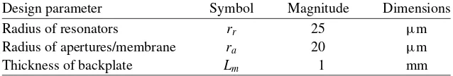
ra=1 nm (solid line), 10 nm (dashed line), 100 nm (dotted line), 1µm (dash dot line) and 25µm (dash dot dot line). The last value being the largest aperture size possible sincerr=25µm, as per Table1. The first value ofra=1 nm should give an indication of how a similar device with no res-onators would operate. Figure5(a) shows the TVR for these five different designs with it being clearly illustrated that the inclusion of resonators with larger apertures (and corresponding larger volumes) results in a higher TVR and a more prominent resonant frequency, although perhaps a reduced band-width. By considering the normalized TVR (Fig. 5(b)) it can be seen that the resonant frequency varies substantially from a sub-ultrasonic resonance (ra=1µm, dash-dot) to resonances in the range of 5−7 MHz. Since there is clearly a high dependence on the aperture radius, it was decided to inves-tigate the dependence of the TVR on the aperture radius for a fixed frequency off =1 MHz. This dependence can be found in Fig.5(c). The figure clearly shows that the TVR is maximized by a value ofra≈12µm.

The RFR follows a similar pattern in all but the resonant frequency positions. Using the same vari-ables as in the TVR case, the results are shown in Fig.6. The results suggest that the device operates in a similar frequency range in the reception and transmission modes; however, it does appear that the device operates substantially better in the reception mode. By varying the aperture size, it seems that the RFR is maximized by a design parameter choice ofra≈12µm. It is also seen that the larger the

(16)

(a)

(b)

(c)

0 1 2 3 4 5

-560 -520 -480 -440

0 2 4 6 8 10

-40 -30 -20 -10 0

0 5 10 15 20 25

0.0 0.2 0.4 0.6 0.8 1.0

transmission voltage response

frequency (MHz)

10nm 100nm 1µm 10µm 100µm

(dB)

frequency (MHz)

transmission voltage response (normalized)

aperture radius (µm)

Fig. 5. TVR (a) and normalized transmission voltage response in dB (b) of the device, for each of the five values for the aperture radius (with corresponding resonator volume). Normalized TVR as a function of aperture radius for fixed frequency f=1 MHz (c).

aperture size, the higher the resonant frequency of the device. However, it should be noted that only the largest aperture size results in an RFR in the ultrasonic range.

4.2 Aperture size with fixed resonator volume

The effect of changing the aperture size, where the volume of the whole resonator is kept constant, is now considered. For ease of comparison, the aperture sizes considered are the same as in the previous section, whereas the volume of the resonator is kept at the same size as in the standard design (calculated via equation (2.9) and Table1). This is clearly not attainable using the chemical set-up described in the introduction to the article, but instead is an interesting mathematical investigation into how the nature of the resonators affects the device’s performance.

[image:16.536.112.413.65.441.2]

(17)

(a)

(b)

(c)

0 1 2 3 4

-300 -275 -250 -225 -200 -175

0.0 0.5 1.0 1.5 2.0 2.5

-40 -30 -20 -10 0

0 5 10 15 20 25

0.0 0.2 0.4 0.6 0.8 1.0

reception force response

frequency (MHz)

1nm 10nm 100nm 1µm 25µm

(dB)

frequency (MHz)

reception force response (normalized)

Fig. 6. RFR (a) and normalized RFR in dB (b) of the device, for each of the five values for the aperture radius (with corresponding resonator volume). Normalized RFR as a function of aperture radius for fixed frequencyf=1 MHz (c).

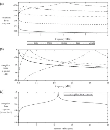
The TVR, normalized TVR and effect of aperture radius for a fixed frequency are given by Fig.7. As can be seen, there are no large differences between these results and those in the previous section, save for the value ofra≈10µm which maximizes the TVR. The same can be said for the RFR, normalized RFR and the effect of aperture radius, given by Fig.8. Both sets of devices operate in the same range of frequencies and both follow similar responses when varying the aperture size. It can therefore be concluded that it is the aperture size which has more influence on the operation of the device than the volume of the resonators.

[image:17.536.93.456.71.502.2]

(18)

(a)

(b)

(c)

0 1 2 3 4 5

-550 -500 -450 -400

0 2 4 6 8 10

-30 -25 -20 -15 -10 -5 0

0 5 10 15 20 25

0.0 0.2 0.4 0.6 0.8 1.0

frequency (MHz)

transmission voltage response (dB)

frequency (kHz)

Fig. 7. TVR (a) and normalized transmission voltage response in dB (b) of the device, for each of the five values for the aperture radius (with fixed resonator volume). Normalized TVR as a function of aperture radius for fixed frequencyf=1 MHz (c).

4.3 Neck length

Finally the effect of constructing a neck on the resonator is scrutinized in order to investigate a possible change in the design which results in an improved bandwidth or resonating frequency. That is, it is not assumed thatL=0 in equation (2.5). To begin, five different lengths of the neck are chosen:L=0 m (solid line), 1µm (dashed line), 10µm (dotted line), 100µm (dash-dot line) and 1 mm (dash-dot-dot line). The TVR and normalized TVR are shown via Fig.9(a,b). These figures show the dependence

[image:18.536.70.443.59.515.2]

(19)

(a)

(b)

(c)

0 1 2 3 4

-300 -270 -240 -210 -180 -150

0.0 0.5 1.0 1.5 2.0 2.5 3.0

-30 -25 -20 -15 -10 -5 0

0 5 10 15 20 25

0.0 0.2 0.4 0.6 0.8 1.0 reception

force response

frequency (MHz)

(dB)

frequency (MHz)

Fig. 8. RFR (a) and normalized RFR in dB (b) of the device, for each of the five values for the aperture radius (with fixed resonator volume). Normalized RFR as a function of aperture radius for fixed frequencyf=1 MHz (c).

of the magnitude, bandwidth and resonating frequency of the device on the length of the neck. It can be seen that the longer the neck, the narrower the bandwidth and the lower the resulting resonating frequency. Figure9(a) also suggests that the highest TVR occurs when the length of the neck is between 10 and 100µm. The actual value of this can be seen easier in Fig.9(c), where the TVR is plotted against the effective length forf =1 MHz. Note thatL≈32µm gives the best TVR. A similar analysis was done for the RFR. Figure10shows the same effect of the resonator neck length on the RFR as the TVR.

[image:19.536.91.454.72.487.2]

(20)

(a)

(b)

(c)

0 1 2 3 4 5

-480 -460 -440 -420 -400

0.0 0.5 1.0 1.5 2.0 2.5 3.0

-60 -40 -20 0

0 20 40 60 80 100

0.0 0.2 0.4 0.6 0.8 1.0 transmission

voltage response

frequency (MHz)

0m 1µm 10µm 100µm 1mm

transmission voltage response (dB)

frequency (MHz)

neck length (µm)

Fig. 9. TVR (a) and normalized transmission voltage response in dB (b) of the device, for each of the five values for the neck length. Normalized TVR as a function of the neck length for fixed frequencyf=1 MHz (c).

5. Conclusions and discussion

This article considered the theoretical modelling of a novel electrostatic transducer in which the back-plate consisted of an array of spherical resonators which act in a similar manner to cavities/pits found in more standard devices. The resonators are made by depositing ternary solutions onto an electrically conducting substrate and the spherical resonators can be created by selective dissolution of one poly-mer phase after phase separation. The dimensions of the cavities and their spatial distribution can be

(21)

(a)

(b)

(c)

0.0 0.5 1.0 1.5 2.0 2.5 3.0

-220 -200 -180 -160 -140

0.0 0.5 1.0 1.5 2.0 2.5 3.0

-70 -60 -50 -40 -30 -20 -10 0

0 20 40 60 80 100

0.0 0.2 0.4 0.6 0.8 1.0

(dB)

frequency (MHz)

0m 1µm 10µm 100µm 1mm

frequency (MHz)

neck length (µm)

Fig. 10. RFR (a) and normalized RFR in dB (b) of the device, for each of the five values for the neck length. Normalized RFR response as a function of the neck length for fixed frequencyf=1 MHz (c).

controlled by selection of the solutes and solvent and the rate of solvent evolution during the deposi-tion process. More specifically, this article focussed on the theoretical modelling of such a device using three different analytical models: a 1D (in space) model, and two 2D (in space) models which consider separate effects on the membrane. The models produced mechanical impedance profiles of the device, in addition to TVRs and RFRs, all of which closely agree.

The 1D pipe-driver model was then used to investigate the effect of changing certain device param-eters on the device performance. Specifically, the aperture radius, resonator volume and aperture neck

(22)

length were varied. It was observed that the resonant frequency, bandwidth and sensitivity of the device were all highly dependent on these resonator parameters.

Each model showed good agreement and illustrated that the device’s performance was highly depen-dent on the parameters of the backplate. It is therefore important to consider an array of resonators to ascertain if their dimensions could be tailored for specific operating frequencies or bandwidths. As an array of exactly similar resonators has the same impedance as one resonator of the same dimensions, then arrays of resonators of varying dimensions should be studied. There is a possibility of being able to compute array designs which produce outputs with much larger bandwidths than the outputs provided herein. The inverse problem of finding the required parameter values which result in a required oper-ating resonance/bandwidth of the device can also be implemented. The models included could also be used as a guideline for constructing a systems-dynamics model which could prove beneficial for finding optimal parameter values for a specific operating bandwidth and resonant frequency.

Some assumptions were made during the modelling which should be addressed. It was assumed, firstly, that the resonators were equally spaced and identical (although the model itself is constructed in such a manner that this need not be the case). Perhaps more importantly, the model assumed that the membrane, while of the order of size of the backplate, has zero displacement everywhere apart from over each aperture, causing the effective radius of the membrane to be much smaller. Clearly, a free membrane would resonate at a much lower frequencies than the resonant frequency of the backplate, meaning that the device would not operate at its desired frequency. These models must be tested against experimental evidence in order to ascertain if the membrane acts in such a manner.

Furthermore, experimental evidence is required to confirm the model’s validity with respect to the operating resonant frequency. In addition, topography scans of the backplate will show to what extent the resonators are of the same shape and dimension. It may be required to introduce a range of sizes of resonators into the model to account for such manufacturing disparities. Furthermore, the actual strength of the pressure output from the models/prototypes must be considered, an aspect which has not been covered in this article. These are experimental issues which are the subject of ongoing investigations.

Finally, there are many facets of these models which could be developed; such as the extent of energy leakage into the silicone substrate and the backplate, the affect of the d.c. bias voltage on device operation and the possibility of filling the resonators with other fluids than air in order to modify the operating frequency. Further methods of comparisons, other than operating frequency, with experimen-tal output will also be considered in future publications.

Acknowledgements

Thanks are given to E. Mackie and R. O’Leary from the Centre For Ultrasonic Engineering, University of Strathclyde, for discussions centred on the experimental work.

Funding

This work was supported by the UK Engineering and Physical Sciences Research Council (EPSRC) (Grant EP/F017421/1). Funding to pay the Open Access publication charges for this article was pro-vided by EPSRC.

References

Álvarez-Arenas, T. E. G. (2004) Acoustic impedance matching of piezoelectric transducers to the air.IEEE Trans.

Ultrason. Ferroelectr. Freq. Control,51, 624–633.

(23)

Bayram, B., Hæggström, E., Yaralioglu, G. & Khuri-Yakub, B. T. (2003) A new regime for operating capacitive micromachined ultrasonic transducers.IEEE Trans. Ultrason. Ferroelectr. Freq. Control, 50, 1184–1190.

Campbell, E.,Galbraith, W. &Hayward, G. (2006) A new electrostatic transducer incorporating fluidic ampli-fication.Ultrasonics Symposium. Vancouver, Canada: IEEE, pp. 1445–1448.

Caronti, A.,Caliano, G.,Iula, A. &Pappalardo, M. (2002) An accurate model for capacitive micromachined

ultrasonic transducers.IEEE Trans. Ultrason. Ferroelectr. Freq. Control,49, 159–168.

Kinsler, L. E.,Frey, A. R.,Coppens, A. B. &Sanders, J. V. (2000)Fundamentals of Acoustics. Chichester: John Wiley.

Ladabaum, I.,Jin, X.,Soh, H. T.,Atalar, A. &Khuri-Yakub, B. T. (1998) Surface micromachined capacitive ultrasonic transducers.IEEE Trans. Ultrason. Ferroelectr. Freq. Control,45, 678–690.

Leighton, T. G. (2007) What is ultrasound?Prog. Biophys. Mol. Biol.,93, 3–83.

Lynnworth, L. C. (1965) Ultrasonic impedance matching from solids to gases.IEEE Trans. Son. Ultrason.,

SU-12, 37–48.

Mackie, E. &O’Leary, R. (2012) Private Communication.

Manthey, W.,Kroemer, N. &Mágori, V. (1992) Ultrasonic transducers and transducer arrays for applications

in air.Meas. Sci. Technol.,3, 249–261.

Noble, R. A.,Jones, A. D. R.,Robertson, T. J.,Hitchins, D. A. &Billson, D. R. (2001) Novel, wide bandwidth, micromachined ultrasonic transducers.IEEE Trans. Ultrason. Ferroelectr. Freq. Control,48, 1495–1507.

Rafiq, M. &Wykes, C. (1991) The performance of capacitive ultrasonic transducers using v-grooved backplates.

Meas. Sci. Technol.,2, 168–174.

Reilly, D. &Hayward, G. (1991) Through air transmission for ultrasonic non-destructive testing.Ultrasonics

Symposium. Orlando, FL: IEEE, pp. 763–766.

Saffar, S. &Abdullah, A. (2012) Determination of acoustic impedances of multi matching layers for

narrow-band ultrasonic airborne transducers at frequencies<2.5 MHz—Application of a genetic algorithm. Ultra-sonics,52, 169–185.

Schindel, D. W.,Hutchins, D. A.,Zou, L. &Sayer, M. (1995) The design and characterization of

microma-chined air-coupled capacitance transducers.IEEE Trans. Ultrason. Ferroelectr. Freq. Control,42, 42–50.

Sneddon, I. N. (1980)Special Functions of Mathematical Physics and Chemistry. London and New York:

Long-man.

Walker, A. J. &Mulholland, A. J. (2010) A theoretical model of an electrostatic ultrasonic transducer incorpo-rating resonating conduits.IMA J. Appl. Math.,75, 796–810.

Walker, A. J.,Mulholland, A. J.,Campbell, E. & Hayward, G. (2008) A theoretical model of a new

electrostatic transducer incorporating fluidic amplification. IEEE Ultrasonics Symposium, Beijing, China, 1409–1412.

Watson, G. N. (1996)A Treatise on the Theory of Bessel Functions, 2nd edn. Cambridge: Cambridge University

Press.

Weisstein, E. W. (2013) ‘Spherical Cap.’ From MathWorld–A Wolfram Web Resource. http://mathworld.

wolfram.com/SphericalCap.html. Accessed 26 August 2013.

Wright, M. C. M. (ed.) (2005)Lecture Notes on the Mathematics of Acoustics. London: Imperial College Press.

Appendix A. Nomenclature

The tables below provide a full nomenclature of terms used within the article. It is worth noting that, as far as notation concerned, the literature is not consistent and care should be taken when comparing with other work.

(24)

Notation Description

Am,Ap Viscous damping

Bm,Bm¯ ,Bp,Bp¯ ,Bpˆ Excitation voltage term

C Capacitance

Cm,Cm¯ ,Cp,Cp¯ , Average displacement of membrane term

C0 Value of capacitanceCatΨ˙ =0

c Speed of sound in resonator

D flexural rigidity of membrane

de Distance between electrodes

dm Thickness of membrane

F Applied force (in frequency domain)

f(t) Voltage driving force (in time domain)

Fe Electrostatic force

fr Force on membrane

G Static conductance

ha Height of removed cap of spherical resonator

I Current at electrical inputs

In Modified Bessel function of first kind ofnth order

i Imaginary number

Jn Bessel function of first kind ofnth order

L Length of neck of resonator

L Effective length of neck of resonator

Lm Distance between lower electrode and membrane

m Total effective mass of aperture

N Number of rows in resonator array

nj Number of resonators in rowj

Pi Amplitude of pressure wave on resonator

Pr Prandtl number

Po Pressure produced at membrane load

pr Pressure in resonator

RFR, (RFR) Reception force response (RFR in decibels)

Rr Radiation resistance of resonator

Rv Damping constant

R_ω Thermoviscous resistance

r Radial variable across resonator aperture

ra Radius of open aperture in resonator

rr Radius of spherical resonator

Sa Area of aperture of resonator

Sm Surface area of membrane

sr Stiffness of resonator

T Transduction coefficient

TVR (TVR) Transmission voltage response (TVR in decibels)

t Time

continued.

(25)

Notation Description

V Applied voltage (time domain)

Vac Alternating current voltage

¯

Vac Applied voltage (frequency domain)

Vdc Direct current voltage

Vr Volume of resonator

xdc Membrane displacement due toVdc

Yn Bessel function of second kind ofnth order

Zb Acoustic impedance of backplate

ZEB Blocked electrical impedance

Zm Mechanical impedance of transducer

Zl

m Mechanical impedance of load

Zb

m Mechanical impedance of backplate

Zr

m Mechanical impedance of resonator

Zmo Open-circuit mechanical impedance atI=0.

Zr _{Acoustic impedance of resonator}

Zs(Zsˆ ) Combined specific acoustic impedance (Zsin decibels)

Zls Specific acoustic impedance of fluid at load Zrs Specific acoustic impedance of resonator

αw Absorption coefficient

β Ratio of transduction coefficient and electrical impedance

γω Attenuation coefficient

r Relative permittivity of the membrane

0 Permittivity of free space

η Coefficient of shear viscosity

λ Wavelength of sound in resonator

ρa Density of fluid in resonator

ρs Density of membrane

τ Tensile strength of membrane

Ψ Displacement of membrane (frequency domain)

ψ Displacement of membrane (time domain)

ω Angular frequency