On boosting kernel regression

promoting access to White Rose research papers

White Rose Research Online

Universities of Leeds, Sheffield and York

http://eprints.whiterose.ac.uk/

This is a final published version of a paper accepted for publication in Journal of Statistical Planning and Inference.

White Rose Research Online URL for this paper:

http://eprints.whiterose.ac.uk/42949/

Paper:

Di Marzio, M and Taylor, CC (2008) On boosting kernel regression. Journal of Statistical Planning and Inference, 138 (8). 2483 -2498.

On boosting kernel regression

Marco Di Marzio and Charles C. Taylor

DMQTE, G.d’Annunzio University, ITALY and Department of Statistics, University of Leeds, UK

Abstract

In this paper we propose a simple multistep regression smoother which is constructed in an iterative manner, by learning the Nadaraya-Watson estimator withL2boosting. We find, in

both theoretical analysis and simulation experiments, that the bias converges exponentially fast, and the variance diverges exponentially slow. The first boosting step is analyzed in more detail, giving asymptotic expressions as functions of the smoothing parameter, and relationships with previous work are explored. Practical performance is illustrated by both simulated and real data.

Key words: Bias Reduction; Boston Housing Data; Convolution; Cross Validation; Local

Polynomial Fitting; Positive Definite Kernels; Twicing.

1 Introduction

1.1 Objectives and motivation

Due to impressive performance, boosting (Schapire, 1990; Freund, 1995) has be-come one of the most studied machine learning ideas in the statistics community.

Basically, a B-steps boosting algorithm iteratively computes B estimates by

ap-plying a given method, called a weak learner, toB different re-weighted samples.

The estimates are then combined into a single one which is the final output. This ensemble rule can be viewed as a powerful committee, which is expected to be significantly more accurate than every single estimate. A great deal of effort is being spent in developing theory to explain the practical behaviour of boosting, and at the moment a couple of crucial questions appear to have been successfully

Email address:

[email protected] and [email protected](Marco Di

addressed. An important question is why boosting works. Now it seems that a sat-isfying response has been provided in that boosting is viewed as a greedy function approximation technique (Breiman, 1997; Friedman, 2001), where a loss function

is optimized by B iterative adjustments of the estimate in the function space; at

each iteration the weighting system indicates the direction of steepest descent. A second question concerns the Bayes risk consistency, and recent theoretical results (Jiang, 2004) show that boosting is not Bayes risk consistent and regularization techniques are needed. Recent results suggest that some regularization methods ex-ist such that the prediction error should be nearly optimal for sufficiently large sam-ples. Jiang (2004) and Zhang and Yu (2005) analyze boosting algorithms with early

stopping, whereas alternative regularization methods are considered by Lugosi and

Vayatis (2004) and by Zhang (2004). In practical applications, a stopping rule is often determined by recourse to cross-validation based on subsamples. However, an alternative more computationally efficient approach, using AIC-based methods, has recently been proposed by B¨uhlmann (2006).

To implement boosting we need to choose a loss function and a weak learner. Ev-ery loss function leads to a specifically shaped boosting algorithm. For example,

AdaBoost (Schapire, 1990; Freund and Schapire, 1996) corresponds to

exponen-tial losses, andL2Boost (Friedman, 2001; B¨uhlmann and Yu, 2003) to L2 losses.

Clearly, if a specific weak learner is considered as well, a boosting algorithm can be explicitly expressed as a multistep estimator, and some statistical properties can thus be derived.

In the present paper we propose a new higher-order biased nonparametric regres-sion smoother that results from learning the Nadaraya-Watson (N-W) estimator

byL2boosting. Note that in polynomial regression bias becomes more serious the

higher the curvature of the regression function. In this latter case the use of a higher polynomial fit — that is asymptotically less biased — is not always preferable since: i) there is no guarantee that the regression function is sufficiently smooth to ensure explicit expressions for the asymptotic bias; and ii) they require much larger samples.

In Section 2 we establish the properties of our boosting algorithm for each itera-tion: exponentially fast bias reduction and exponentially slow variance inflation are

proved. In Section 3 we explore the asymptotic behaviour (asn _{→ ∞}) in the first

1.2 L2boosting

In what follows a description of L2boosting suitable for our aims is given; more

details can be found in the references.

Given three real random variables, X, Y and ε assume the following regression

model for their relationship

Y =m(X) +ε, with Eε= 0, var ε=σ2, (1)

where X and ε are independent. Assuming that n i.i.d. observations S :=

{(Xi, Yi), i = 1, ..., n_} drawn from (X, Y) are available, the aim is to estimate

the mean response curve m(x) = E(Y _| X = x). Note thatm(x) = r(x)/f(x)

where r(x) := R yg(x, y)dy, f(x) := R g(x, y)dy and g is the joint density of

(X, Y). This is the random design model, in the fixed design model we have a

set of fixed, ordered points, x1, . . . , xn that are often assumed equispaced, so the

sample elements ares:= (xi, Yi;i= 1, ..., n).

L2boosting is a procedure of iterative residual fitting where the final output is

simply the sum of the fits. Formally, consider a weak learner _M that is a crude

smoother. An initial least squares fit is denoted by_M0. For b ∈ [1, . . . , B], Mb

is the sum of _Mb−1 and a least squares fit of the residuals Se := {Xi, ei :=

Yi− Mb−1(Xi)}. TheL2boosting estimator isMB.

Typically, the minimal loss obtainable over all boosting iterations, will be achieved

after a finite number of iterations. Actually, the moreBincreases, the more_MB

be-comes complex and tends to closely reproduce the sample (overfitting). Therefore, a stopping rule is needed.

2 L₂boosting and local polynomial fitting

2.1 Local polynomial andL2boosting

Givenp, usually0,1or2, to estimatem(x)we could solve

min

β0,...,βp

n X

i=1  

Yi−

p X

j=0

βj(Xi₋x)j

   2

Kh(Xi₋x) (2)

by fittingPp_j=0βj(_{· −}x)j toS. This givesmd(j)_{(x;S, h) :=j!βj}b _{. Here, the weight}

functionKh(·) := K(·/h)/his non-negative, symmetric and unimodal, andh >0

smoothers (see, for example, Fan and Gijbels, 1996). As mentioned in Section 1.1,

the use of a p-degree polynomial is meaningful only when m(p+1)_{(x)exists; this}

constraint is regarded as the most severe required by this approach.

Notice that md(j)_{(x;S, h) is a least squares fit, so each pair h and p identifies a}

weak learner forL2boosting. But how to selectp? It is known that for a successful

implementation of boosting we need a weak learner. Now within the class of the

local polynomial smoothers the casep= 0— called the N-W smoother — can be

regarded as crude because it is the simplest polynomial (a constant term) to employ

in the fit of the Taylor series expansion ofm.

2.2 The Nadaraya-Watson smoother andL₂BoostNW

Given a sampleS, we want to estimatem(x)in model (1). The N-W estimator is

c

mNW(x;S, h) :=

n−1Pn

i=1Kh(x−Xi)Yi n−1Pn

i=1Kh(x−Xi)

which, as stated, is the solution of Equation (2) when p = 0. For the simplest

interpretation, note that a N-W fit is a locally weighted average of the responses.

Now we recall a bias approximation of cmNW(x;S, h)useful for the next section.

H¨ardle (1990) gives a detailed treatment of the subject.

Let this usual set of conditions hold

(1) x is an interior point of the sample space, i.e. inf(suppf) + h _≤ x _≤

sup(suppf)₋h;

(2) mandf are twice continuously differentiable in a neighbourhood ofx;

(3) the kernelKis a symmetricPDF;

(4) h_→0andnh_{→ ∞}asn_{→ ∞};

(5) f′′_{is continuous and bounded in a neighbourhood ofx.}

Indicate by rˆ(_·;S, h)and fˆ(_·;h) the numerator and denominator ofmˆNW(·;S, h),

respectively. Using condition (4), it has been shown that the leading term of a large sample approximation givesEcmNW≈Er/b Efb. It is easy to show that

Erb(x;S, h) =r(x) + h

2

2 µ2r

′′_{(x) +O(h}4_{); (3)}

whereµk:=R vk_{K(v)dv, and that}

Efb(x;h) =f(x) + h

2

2µ2f

Therefore, the bias is of orderO(h2_{), in particular:}

m(x)₋cmNW(x;S, h)≈

h2_µ 2

2f(x){r

′′_(x)−m(x)f′′_{(x)}. (5)}

We proposeL2boosting with the N-W estimator as our weak learner using the

fol-lowing pseudocode:

Algorithm:L2BoostNW

1. (Initialization) Given Sandh >0, (i) mc0(x;h) :=mcNW(x;S, h).

2. (Iteration) Repeat forb= 1, ..., B

(i) ei :=Yi −mbc−1(Xi;h) i= 1, ..., n;

(ii) cmb(x;h) := mbc−1(x;h) + mcNW(x;Se, h), where Se = {(Xi, ei), i =

1, . . . , n_}.

2.3 Properties ofL2BoostNW

Let(x1, y1), ...,(xn, yn)be data from model (1), the Nadaraya-Watson estimates at the observation points are compactly denoted as

c

m₀ =N Ky

where mcT₀ := ( ˆm0(x1;h), ...,mˆ0(xn;h)), N−1 := diag({Pni=1Kh(x1 − xi)_}, . . . ,_{Pn_i=1Kh(xn ₋xi)_}), yT := (y1, ..., yn) and (K)ij := Kh(xi − xj).

Notice that this fit is linear, but unfortunately the hat matrixN Kis not symmetric,

therefore the detailed theory established by B¨uhlmann & Yu (2003) forL2boosting

of symmetric learners is not applicable here. Indicate asspec(A)the set of the

char-acteristic roots of the square matrixA. It will be apparent thatL2BoostNW works

properly only ifspec(N K) _⊂ (0,1]; in Theorem 1 we define a class of kernels

satisfying such a property. In Theorem 2 we give finite sample accuracy measures ofL2BoostNW at stepb≥0.

Theorem 1 If the continuous second-order kernelK is

1) a Fourier-Stieltjes transform of a finite measure; and 2) symmetric and unimodal;

thenspec(N K)_⊂(0,1]. Moreover,min spec(N K)<1.

Proof: See the Appendix.

Triweight do not. This is somewhat surprising, in view of the fact that the kernel

choice is often influenced by computational convenience.

Now define the mean squared error ofL2BoostNW, averaged over the observation

pointsx1, ..., xn, as

ave-MSE(mcb;m, σ2) := ave-bias2(mcb;m) +ave-var(mcb;σ2),

where mT _{:= (m(x}

1), ..., m(xn)) is the vector of the regression function at the observation points,

ave-bias2(mcb;m) :=

1

n n X

i=1

(Ecmb(xi;h)₋m(xi))2,

and

ave-var(mc_b;σ2_{) :=} 1 n

n X

i=1

varcmb(xi;h).

Theorem 2 Let(x1, y1), ...,(xn, yn)be data from model (1), then

ave-bias2(mc_b;m) = 1

nm

T_(U−1₎T_{diag((1−λk)}b+1_)UT_{Udiag((1−λk)}b+1_)U−1_m,

ave-var(mcb;σ2) = σ2

n trace{Udiag(1−(1−λk)

b+1_)U−1_(U−1₎T_{diag(1−(1−λk)}b+1_)UT_}.

where λ1, ..., λn are the characteristic roots of N K, b ≥ 0, and U is a n ×n invertible matrix of real numbers.

Moreover, ifspec(N K)_⊂(0,1], then

lim

b→∞

ave-bias2(mc_b;m) = 0,

lim

b→∞

ave-var(mc_b;σ2_{) = σ}2_,

lim

b→∞

ave-MSE(mcb;m, σ2) = σ2;

ave-bias2 converges exponentially fast, whileave-varconverges exponentially slow.

Proof: See the Appendix.

For a given stepb, the bias-variance tradeoff emerges: increased characteristic roots

correspond to a bandwidth reduction, with obvious consequences. But it is also

apparent that, if Theorem 1 holds, for eachk_∈[1, ..., n]we have

lim

h→0(1−λk)

b+1 _{= lim}

b→∞(1−λk)

this suggests that bandwidth selection needs to be accomplished by taking into

account the boosting iterations planned. However, as in the case of L2boosting of

symmetric learners (B¨uhlmann & Yu (2003)), the bias decreases exponentially fast

towards zero, while variance increases exponentially slow towardsσ2_{, which shows}

a resistance to overfitting.

3 The first boosting step (B= 1)

3.1 L2BoostNW reduces the bias of the N-W estimator

In this Section we consider the asymptotic bias and variance at the first boosting step. This is an alternative perspective to the one used in the previous section in which conditional expectations were obtained for finite samples.

Theorem 3 Assuming conditions (1)–(5) hold, after the first boosting step we have

Ecm1(x;h) = m(x) +o(h2),

varcm1(x;h) ≤ 4varcm0(x;h).

Proof: See the Appendix.

As a consequence, we observe a reduction in the asymptotic bias from O(h2_{) in}

Equation (5) to o(h2_{)above. This conclusion is consistent with that found by Di}

Marzio and Taylor (2004, 2005), where boosting kernels gives higher order bias for both density estimation and classification. More generally, bias reduction was noted by Friedman et al. (2000) when considering Adaboost. Since at the first step the magnitude order of the variance is preserved, then the mean squared error is

reduced provided thatnis sufficiently large.

3.2 Links to previous work

3.2.1 Twicing and higher order kernels: theory

out that twicing for kernel regression in a fixed, equispaced design is

c

mSM(x;s, h) := 2n−1

n X

i=1

Kh(x−xi)Yi−n−1 n X

i=1

Kh(x−xi) n X

j=1

Kh(xi−xj)Yj

where x1 = 0 and xn = 1. They observed that the second summand contains

a discretization of a convolution of the kernel with itself. Thus, for a sufficiently

fine, equispaced, fixed design twicing approximates the estimatorcmSM(x;s, h) =

n−1P_K∗

h(x−xi)YiwithKh∗ := 2Kh−(K∗K)h. (The convolution between pdfs f andg is(f _∗g)(x) := R f(x₋y)g(y)dy.) Now note thatK∗

h is a higher order

kernel, here called the convolution kernel, consequentlycmSM is a higher order bias

method.

Note that although both are higher order biased,cmSM is defined only for the fixed

equispaced design case, while cm1 is indifferent to the design. An obvious

ques-tion concerns the possibility of extendingmSMc to the random design, and so we

will compare — both theoretically and numerically — the performance of such

an extension with cm1. Assume that Kh is a normal density with mean zero and

standard deviationh, denoted as φh, because in this case the convolution is simply

(φ_∗φ)h =φ√2h. There are two main options of implementing twicing by using the

convolution kernel:

c m∗

1(x;S, h) := Pn

i=1φ∗h(x−Xi)Yi

Pn

i=1φ∗h(x−Xi)

=

Pn i=1

n

2φh(x₋Xi)₋φ√

2h(x−Xi) o

Yi Pn

i=1 n

2φh(x₋Xi)₋φ√

2h(x−Xi) o

c m∗

2(x;S, h) := 2

Pn

i=1φh(x−Xi)Yi Pn

i=1φh(x−Xi)

−

Pn

i=1φ√2h(x−Xi)Yi Pn

i=1φ√2h(x−Xi)

in whichcm∗

1can be viewed as the closest one tocmSM. It simply amounts to dividing

c

mSM — that is a consistent estimator ofr— by a density estimate: it is a ‘higher

order N-W’ smoother derived from a ‘higher order Priestley-Chao’ one. Surelycm∗

2 appears a more direct implementation of the twicing idea and is most similar to

c

m1. We can compare each of these tomc1, and all three estimators can be compared

(bias and variance etc.) with the true regressionmin simulations.

Denote the numerator and denominator of cm∗

1(x;h) by rb1∗(x;h) and fb1∗(x;h). Na¨ıvely plugging these in to equations (3) and (4) we would get

Emc∗

1(x;S, h) = (

2r(x) +h2µ2r′′(x)−r(x)−

(√2h)2

2 µ2r

′′_{(x) +o(h}2₎ )

×

(

2f(x) +h2f′′_{(x)−f(x)−} (

√ 2h)2

2 µ2f

′′_{(x) +o(h}2₎

)−1

=m(x) +o(h2)

and theO(h2_{)bias terms appears to have been eliminated. However, we note that,}

since fb∗

longer valid. Although the numerator and denominator become zero at the same time, the denominator can take negative values while the numerator is positive, so the estimator will be very unstable.

Secondly, if we use equation (5) to obtainEmc∗

2we get

Ecm∗

2(x;S, h) = 2EmcNW(x;S, h)−EcmNW(x;S,

√ 2h) =m(x),

and so theO(h2_{)bias term is apparently eliminated for this estimator also.}

3.2.2 Twicing and higher order kernels: some simulations

Our objective here is to compare the estimators and their ability to reduce bias in different parts of the sample space. We will adopt the experimental design of Hastie and Loader (1993) who considered adaptive kernels for use at the boundary.

Specifically, we taken = 50 points which are (i) equispaced, and (ii) X _∼ f(x)

withf(x) = 6x(1₋x)I[0,1](x). For eachxi we generateYi = x2i +εi with εi ∼

N(0,1). Given h we can estimate the mean integrated squared error MISE cm =

ER (cm₋m)2for each estimatorcm, including the basic N-W estimator.

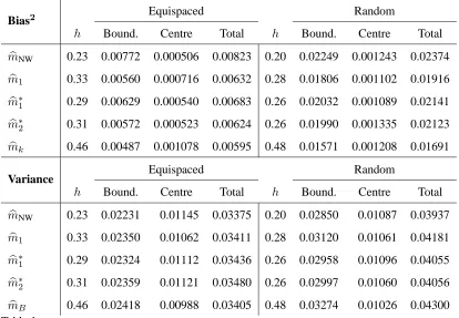
In Table 1 we give the mean integrated squared bias, and the mean integrated vari-ance corresponding to the optimal choice of smoothing parameter — to minimize MISE over the full range — for each estimator. In the case of boosting, the number

of iterations was optimized over all pairs (h, b). As in Hastie and Loader (1993),

we give a breakdown according to the interior, and center of the range [0,1]. The

results are estimated from 200 simulations of sample sizen= 50.

It can be seen that most of the MISE is due to the contribution at the boundaries, particularly the bias-squared, which is an order of magnitude greater. All three bias reduction methods make most of their impact in the boundary contribution, with the bias showing a substantial decrease and only a modest increase in variance, with an overall reduction in MISE compared with the standard N-W estimator. For

this example, it seems thatcm1 (boosting one iteration) is the best single iteration

method for both equispaced and random design data. However, we note that the bias is not as small — even after several boosting iterations — as that obtained by Hastie and Loader (1993) for their local linear regression estimator, which used an adaptive smoothing parameter near the boundaries.

4 Simulation study (B _≥1)

In this section we report the conclusions of a simulation study which verifies the

Bias2 Equispaced Random

h Bound. Centre Total h Bound. Centre Total

b

mNW 0.23 0.00772 0.000506 0.00823 0.20 0.02249 0.001243 0.02374

b

m1 0.33 0.00560 0.000716 0.00632 0.28 0.01806 0.001102 0.01916

b

m∗

1 0.29 0.00629 0.000540 0.00683 0.26 0.02032 0.001089 0.02141

b

m∗

2 0.31 0.00572 0.000523 0.00624 0.26 0.01990 0.001335 0.02123

b

mk 0.46 0.00487 0.001078 0.00595 0.48 0.01571 0.001208 0.01691

Variance Equispaced Random

h Bound. Centre Total h Bound. Centre Total

b

mNW 0.23 0.02231 0.01145 0.03375 0.20 0.02850 0.01087 0.03937

b

m1 0.33 0.02350 0.01062 0.03411 0.28 0.03120 0.01061 0.04181

b

m∗

1 0.29 0.02324 0.01112 0.03436 0.26 0.02958 0.01096 0.04055

b

m∗

2 0.31 0.02359 0.01121 0.03480 0.26 0.02997 0.01060 0.04056

b

mB 0.46 0.02418 0.00988 0.03405 0.48 0.03274 0.01026 0.04300

Table 1

Best MISEs decomposed for several kernel regression estimators: m_bNW — standard Nadaraya-Watson;m_b1 — twicing;mb∗i, i = 1,2— higher order kernel methods;mbB with

B = 4,6 (optimal) boosting iterations of L2BoostNW for equispaced and random

spac-ing, respectively . Integrated bias-squared and variance evaluated over the boundary region [0,0.3)_∪(0.7,1], and centre region[0.3,0.7]for fixed (equi-spaced) design, and random de-sign pointsxi, i= 1, . . . ,50. Averages taken over200simulations, with bandwidth chosen

to minimize MISE in each case.

we defer the selection of the bandwidth and number of boosting iterations, and present the performance that each method gives when the bandwidth is optimally selected. Results which use a cross-validation selection of the required parameters will be discussed in section 5.

Our study is made of two parts. The first one is aimed to illustrate the general

performance of L2BoostNW as a regression method per se; here we have chosen

the models used by Fan and Gijbels (1996, pg. 111). In the second part we compare

L2BoostNW with the L2boosting regression method proposed by B¨uhlmann and Yu (2003) using their simulation model. This comparison is particularly interesting because their method is closely related to ours, in that they learn a nonparametric

4.1 General performance

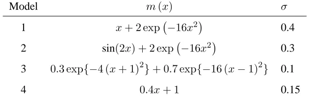
Fan and Gijbels (1996) characterize their case studies as difficult estimation prob-lems due to the level of the noise to signal ratio values. Consider model (1) with

ε normally distributed; the simulation models are specified in Table 2, where, as

Model m(x) σ

1 x+ 2 exp ₋16x2 0.4

2 sin(2x) + 2 exp ₋16x2 0.3

3 0.3 exp_{−4 (x+ 1)2_}+ 0.7 exp_{−16 (x₋1)2_} 0.1

4 0.4x+ 1 0.15

Table 2

The simulation models of Fan and Gijbels (1996).

suggested by Fan and Gijbels, a random design was adopted: for models 1, 2 and 3

X _∼ U(₋2,2)and for model4X _∼ N(0,1).We performed simulations for

sam-ple sizes50,100and200. In Figure 1 we have plotted the integrated mean squared

error forn = 50 for various values of(h, B). The plots confirm that boosting can

reduce the MISE if the smoothing parameter is chosen correctly. Numerical sum-maries are given in Table 3, which also include information for other sample sizes.

This Table shows the best MISEs (calculated from 200 samples) of L2boosting

with the N-W smoother as the weak learner, as well as the gain in MISE which can be achieved by boosting with respect to the N-W estimator.

The results for model 4 suggest that a very large smoothing parameter, together with very many boosting iterations, are preferred for data which are generated by

a straight line. In Figure 2 we plot the estimates cmb(x;h) for various values of

b, and then compare the values cm255(x;h),cm1000(x;h) and cm10000;h(x) with the

true model and the standard (OLS) regression line. It can be seen that the effect of boosting has given a very similar result to a nonparametric polynomial fit with

degreep = 1. This approximation seems to hold true of the other models as well,

but we have preferred this example because it shows that boosting fixes one of the main problems of the N-W smoother i.e. — as pointed out by M¨uller (1993)

— the difficulty of estimating straight regression lines when X is not uniformly

distributed.

4.2 Comparison with boosted splines

The simulation model used by B¨uhlmann and Yu (2003) is specified by

0.10 0.15 0.20 0.25 0.25 0.30 0.35 0.40 0.45

Model 1; n=50

bandwidth MISE 1 2 3 4 5 6

0.10 0.15 0.20 0.25

0.15

0.20

0.25

0.30

0.35

Model 2; n=50

bandwidth MISE 1 2 3 4 5 6 7

0.08 0.10 0.12 0.14 0.16 0.18 0.20 0.22

0.020

0.025

0.030

Model 3; n=50

bandwidth MISE 1 2 3 4 5 6

0 1 2 3 4 5

0.0

0.2

0.4

0.6

0.8

Model 4; n=50

bandwidth MISE 1 2 4 8 16 32 64

Fig. 1. MISEs forn = 50 for each of the four models given in Table 2. These are given as a function of the smoothing parameter for various values ofB = 1,2,3, . . .as shown in the plots). The points (joined by a dashed line) are the optimal values (overh) for eachB.

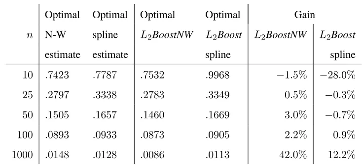
They estimatem(x)by using splines as the weak learner inL2Boost with 100

sam-ples drawn for each of four sample sizes. The accuracy criterion is equivalent to MISE and is estimated in the usual way. The values are summarized in Table 4, where the results of the original study are also shown. Note that both methods are optimized over their relevant parameters and so the comparison should be

mean-ingful. For very small sample sizesL2boosting is outperformed by its base learner:

marginally in the case of N-W; dramatically in the case of splines. In fact, our results are uniformly better for all sample sizes, and although our base learner is

asymptotically inferior to splines, for all n L2BoostNW outperforms the boosted

Model m_bNW p= 1 p= 2 L2BoostNW gain

n= 50 h MISE h MISE h MISE MISE k h

1 .13 .2477 .17 .2909 .29 .3367 .2268 3 .20 8.4%

2 .1 .1841 .15 .2101 .26 .2459 .1482 4 .19 19.5%

3 .1 .0196 .15 .0250 .27 .0286 .0167 4 .19 14.8%

4 .25 .0205 6∗ _{.0044 4}∗ _{.0068 .0049 70* 3.3* 76.1%}

n= 100

1 .12 .1247 .12 .1346 .20 .1383 .1104 4 .19 11.5%

2 .09 .0866 .10 .0907 .18 .0898 .0687 6 .19 20.7%

3 .09 .0095 .10 .0101 .19 .0104 .0077 6 .19 19.0%

4 .21 .0101 10∗ _{.0019 4}∗ _{.0029 .0021 200* 5.3* 79.3%}

n= 200

1 .09 .0658 .10 .0683 .16 .0642 .0557 5 .14 15.4%

2 .07 .0439 .08 .0445 .15 .0401 .0334 7 .18 24.0%

3 .07 .0049 .08 .0050 .15 .0045 .0037 8 .18 24.5%

4 .14 .0059 10∗ _{.0011 4}∗ _{.0014 .0011 164-927 6.0* 81.4%}

Table 3

Simulation results from boosting kernel regression using Fan & Gijbels models shown in Table 2. Gain is percentage improvement of the best boosting estimate over the best N-W smoothing, p = 1,2 correspond to local polynomial fitting using Equation (2); ∗ = boundary values of the grid used.

−3 −2 −1 0 1 2 3

0.0

0.5

1.0

1.5

2.0

estimated curves for model 4, bandwidth=5

x

estimate

0 1 3 7 15 31 63 127 255

−3 −2 −1 0 1 2 3

0.0

0.5

1.0

1.5

2.0

boosting estimate at iteration 255, 1000, 10000

x

estimate

Optimal Optimal Optimal Optimal Gain

n N-W spline L2BoostNW L2Boost L2BoostNW L2Boost

estimate estimate spline spline

10 .7423 .7787 .7532 .9968 ₋1.5% ₋28.0%

25 .2797 .3338 .2783 .3349 0.5% ₋0.3%

50 .1505 .1657 .1460 .1669 3.0% ₋0.7%

100 .0893 .0933 .0873 .0905 2.2% 0.9%

1000 .0148 .0128 .0086 .0113 42.0% 12.2% Table 4

L2BoostNW performances when estimating the model used by B ¨uhlmann and Yu (2003).

The performances of smoothing splines andL2Boost used by B ¨uhlamnn and Yu (2003) are

also reported.

4.3 Optimal values ofhandB

The result in Equation (6) suggest thathneeds to increase withB. The case

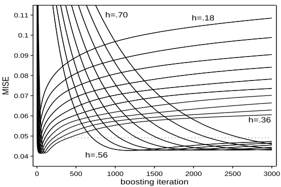
stud-ies of Fan and Gijbels depicted in Figure 1 unequivocally suggest that boosting reduces oversmoothing effects if intensively iterated. Here we illustrate this by a new, ad hoc example based on the model used by B¨uhlmann and Yu. We drew

200 samples withn = 200and estimated the regression function for various

band-widths and boosting iterations. The accuracy results are shown in Figure 3, where

many MISE/iteration curves are depicted. The best MISE occurs whenh _≈ 0.2,

but values quite close to this occur for each setting of the bandwidth. Remarkably, note that when the bandwidths are around 3–3.5 times bigger than 0.2, nearly op-timal MISEs are reached after several hundreds of iterations, and moreover the

best N-W estimate is always beaten forB > 700! Finally, Figure 3 also suggests

how bandwidths of the same magnitude work similarly, another reason to conclude that boosting is less sensitive to the bandwidth selection task than standard kernel regression.

Overall, note that regularizing through oversmoothing in conjunction with many

iterations increases the combinations of (h, B) for which boosting works. Thus,

the potential of reducing the need of an accurate bandwidth selection and stopping rule clearly emerges.

5 Application to multidimensional real data

0 500 1000 1500 2000 2500 3000 0.04

0.05 0.06 0.07 0.08 0.09 0.1 0.11

boosting iteration

MISE

h=.18

h=.36 h=.70

h=.56

Fig. 3.L2BoostNW estimates of the B ¨uhlmann and Yu model. MISEs forn= 200given

as a function of boosting iteration for various values ofh. Dotted line: best MISE of the N-W estimator.

and the number of boosting iterations by cross-validation. We extend our smoother in the most usual way, that lies in building multiplicative kernels with a diagonal bandwidth matrix. In particular, with D-dimensional data (x₁, y1), . . . ,(xn, yn), we employ, with obvious notation, the following weight function

D Y

d=1

Kh(xd−xid).

We use the normal kernel function because this ensures that the conditions of The-orem 1 hold in the multivariate setting.

We obtain(hCV, BCV)by leave-one-out cross-validation, i.e. as the pair that solves

min

h,b = n X

i=1

yi₋mc(−_b i)(x_i;h)2, (7)

wheremc(−_b i)(xi;h)is theL2BoostNW estimate ofm(xi)when theith observation

is omitted.

number of variables could lead us to believe.

MSE MSEopt hCV hopt BCV Bopt

local linear 0.1593 0.1504 2.00 2.55

b

mNW 0.2575 0.2553 0.55 0.50

L2BoostNW 0.1525 0.1477 2.00 1.70 119 115

parametric linear 0.3340 Table 5

Results from the Boston housing data.

Since we are using a common smoothing parameter for all variables, we have stan-dardized the data. We randomly chose 350 instances as a training set, and the

re-maining data as a test set. The accuracy criterion was the mean squared error (MSE)

on the test data. As a benchmark we used the plain N-W estimator, the local linear

polynomial estimator (the solution of Equation (2) when p = 1) and a standard

parametric linear model. Each cross-validation search of h was performed in the

interval[0,3]. The results are summarized in Table 5. The parametric linear fit has

a MSE of 0.3340, suggests that a certain linearity is present in the data. This

ap-pears confirmed by the good performance of the local linear estimator that yields

an accuracy of 0.1593which outperforms the N-W fit. Concerning our multistep

estimator, the cross-validation search of a pair(h, B)was performed over the grid

[0,1, . . . ,3]_×[1,2, . . . ,200], with a MSE of 0.1525. It is clear from Table 5 that

L2BoostNW performs well in higher dimensions, and that cross-validation can be

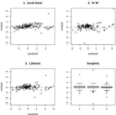
used to successfully obtain the pair(h, B). Residual plots, shown in Figure 4

con-firm this view. Note also that these accuracy values appear quite similar to the results from model 4 of Table 3 where a univariate linear model was estimated, so our estimator seems to coherently extend its properties to the multivariate setting. Another interesting issue is that the cross-validation search was very precise,

be-cause forB _≤ 200the best possible MSE of our boosted estimator is0.1477, and

the optimal setting of(h, B)is very similar to the cross-validation solution.

−1 0 1 2

−3

−2

−1

0

1

2

3

1. local linear

predicted

residual

−2 −1 0 1 2 3

−3

−2

−1

0

1

2

3

2. N−W

predicted

residual

−2 −1 0 1 2 3

−3

−2

−1

0

1

2

3

3. L2boost

predicted

residual

1 2 3

−3

−2

−1

0

1

2

3

method

boxplots

Fig. 4. Residual plots of the Boston housing test data corresponding to the three best models in Table 5.

6 Discussion

6.1 Alternative generalizations

LethT _{:= (h}

0, . . . , hB),wT := (w0, . . . , wB)be vectors of smoothing parameters and weights respectively, then

Kwh :=

B X

j=0 wjKhj

is a weighted sum of kernel functions. The convolution kernel used in Section 3.2 is

We can thus generalizecm∗ 2 to

c

mg(x;S,w,h) := B X

j=0

wjmcNW(x;S, hj). (8)

This is simply a linear combination of N-W estimators, each with its own band-width. Similar proposals were considered by Rice (1984) and Jones (1993) who used weighted combinations of kernels to improve estimators at the boundary. In

order formgc to be asymptotically unbiased we require Pwj = 1. Given a vector

of bandwidthshwe can choose thewj to eliminate the bias terms which arise as a

consequence ofµk.

Since we have used a normal kernel, for a given bandwidthhwe have µ2k ∝ h2k,

and µ2k−1 = 0 so a simple approach to obtain the weights wj would be to set

hT _{= (h,}√_{ch, . . . , c}B/2_{h)for somec, and then to solveCw = (1,0, . . . ,0)}T _for

w, where (forB _≥1)

C =

         

1 1 _{· · ·} 1

1 c _{· · ·} cB

..

. ... ... ...

1cB _{· · · c}2B−1          

and this simplification requires the selection of only two parameters (candh), for

a given B. Note that the above convolution kernel K∗

h uses c = 2, and that the

solution forwgives the desired value(2,₋1).

As an alternative approach, we could consider obtaining thewj by ordinary least

squares regression, i.e. obtain w from wc := (XT_X)−1_XT_{Y where Y}T _:=

(Y1, . . . , Yn) is the vector of responses, and the jth column of the matrix X is given by(cmNW(X1;S, hj), . . . ,cmNW(Xn;S, hj))

T

. This approach could also allow

for the selection ofBthrough standard techniques in stepwise regression. Also note

the connection between (8) and a radial basis function (RBF) representation. In this

framework thewjare the weights, andmNW(x;S, hj)act as “basis functions” which

are themselves a weighted sum of basis functions. So this formulation is equivalent

to a generalizedRBFnetwork, in which an extra layer is used to combine estimates,

but with many of the weights being fixed.

6.2 Conclusions

We have discussed a multistep kernel regression smoother generated by learning

the N-W estimator byL2boosting. Our main result is that the bias ofL2BoostNW

decreases exponentially fast towards zero, while the variance increases

of the ordinary kernel methods in regression. Our experiments show that this

su-periority occurs for several settings of (h, B), and also that cross-validation can

be successfully used for parameter selection. It is clear that the optimal bandwidth for boosting is greater than the values provided by the standard selection theories. Finally, note that our method is easily extended to multivariate data.

Acknowledgements

The authors are grateful to the Associate Editor and two anonymous referees for their valuable comments which led to considerable improvements in this article.

Appendix

Proof of Theorem 1: Following Bochner’s theorem (see e.g. Lax, 2002, p. 144),

spec(K) _⊂ [0,+_∞) if and only if K is a Fourier-Stieltjes transform of a finite

measure. Due to symmetry and unimodality,Kh(0) > Kh(xi ₋xj)for each i ₆=

j, so detK > 0. Clearly, spec(N1/2KN1/2) = spec(N K), but N K is row

stochastic, so apply the Perron-Frobenius theorem for which

1 =min

i { n X

j=1

(N K)ij} ≤max spec(N K)≤max i {

n X

j=1

(N K)ij}= 1

and conclude that spec(N K) _⊂ (0,1]. Finally, trace(N K) < n yields

min spec(N K)<1.

Lemma 1 (B ¨uhlmann & Yu, 2003) Consider linear smoothing by a hat matrixL

with characteristic rootsρ1, ..., ρn. OperateL2boosting with weak learnerL. Then L2boosting at stepb≥0is a linear smoother as well, whose hat matrix is equal to

I₋(I ₋L)b+1_.

Proof: The residual vector at stepb _∈[1, ..., B], denoted ase_b, can be written as

eb =y−mcb−1 =eb−1−Leb−1 = (I −L)eb−1

implyinge_b = (I₋L)b_{yforb ∈[1, ..., B]. Sincemc}

0 =Ly, using a telescope-sum

argument, we obtain

c

m_b =

b X

j=0

Proof of Theorem 2: From Lemma 1 it follows that theL2BoostNW fit ismcb =

Mby. Now, the hat matrixMbcan be written as

Mb =U DbU−1

whereD_b := diag(1₋(1₋λ1)b+1, ...,1−(1−λn)b+1);λ1, ..., λn, are the

char-acteristic roots of N K, which are real due to theorem 1. As a consequence, the

matrixU, formed by the characteristic vectors ofMb, has real entries. Notice that

N K is not symmetric, thereforeU UT ₆=I. Now

bias2(mcb;m) = (E[Mby]−m)T(E[Mby]−m)

= ((M_b−I)m)T((M_b−I)m)

where

Mb−I =U(Db −I)U−1

=Udiag(₋(1₋λ1)b+1, ...,−(1−λn)b+1)U−1.

The covariance matrix is

cov(Mby) = Mbcov(y)MbT =σ2MbMbT =σ2U DbU−1(U−1)TDbUT,

so the variance is

var(mcb;m) =trace(cov(Mby)).

Assume thatspec(N K) _⊂ (0,1]. For anyk _∈ [1, ..., n]the bias order isO_{(1₋

λk)b+1_{}, while the variance order is O{(1− (1− λk)}b+1₎2_{}. So bias converges}

exponentially fast and variance converges exponentially slow.

Proof of Theorem 3: We have

c

m1(x;h) =

2rb(x;h)₋n−1Pn

i=1Kh(x−Xi)cm0(Xi;h) b

f(x;h) .

Now take the expectation of the numerator and denominator. The expectation of the second term in the numerator can be written as

E [Kh(x₋X1)mc0(X1;h)] = E 

 1

nhKh(x−X1) n X

j=1

Kh(X1−Xj)Yj .

b

f(X1;h)  

= 1

h ZZZ

Kh(x₋u)Kh(u₋v)yf(y_|v)

×

(

f(u) + h

2

2 µ2f

′′_{(u) +o(h}2₎

)−1

f(u)f(v)dy du dv

= 1

h ZZ

Kh(x−u)Kh(u−v)m(v)

×

(

1 + h

2_µ 2f′′(u)

2f(u) +o(h

2₎

)−1

where the second line was obtained by ignoring the non-stochastic term in the sum (whenj =i), and the third one uses the fact thatm(v) =Ryf(y_|v)dy.

Making the change of variablet = (v₋u)/hand expandingm(v) = m(u+ht)

andf(v) = f(u+ht)in a Taylor series we get the following expansion up to terms

of orderO(h2₎

E [Kh(x₋X)cm0(X;h)]≈ ZZ

Kh(x₋u)K(t)

(

m(u) +thm′_{(u) +} t

2_h2_m′′_(u)

2

)

×

(

1₋ h

2_µ 2f′′(u)

2f(u)

) (

f(u) +thf′_{(u) +} t

2_h2_f′′_(u)

2

) dt du

=

Z

Kh(x₋u)

"

r(u) + h

2_µ 2

2 {r

′′_(u)−m(u)f′′_(u)} #

du

(9)

=r(x) +h2µ2r′′(x)− h2_µ

2

2 m(x)f

′′_{(x). (10)}

The RHS of Equation (9) was obtained on simplification and recalling thatr′′_{(u) =}

m′′_{(u)f(u) + 2m}′_(u)f′_{(u) +m(u)f}′′_{(u); the RHS of Equation (10) has been}

ob-tained by making a second change of variable w = (x ₋u)/h, expanding in a

Taylor series, and integrating.

To obtain the expectation of the numerator ofcm1(x;h), we multiply Equation (3)

by2, then subtract the RHS of Equation (10) to get

E

"

2rb(x;h)₋ 1

n n X

i=1

Kh(x₋Xi)cm0(Xi;h) #

≈r(x) + h

2_µ 2

2 m(x)f

′′_(x).

Finally we divide this by the approximate (up to the second order) expectation of

the denominator ofcm1(x;h)which is given in Equation (4). We can thus write the

following expression for the asymptotic expectation up to terms of orderO(h2₎

Ecm1(x;h)≈ (

r(x) + h

2_µ 2

2 m(x)f

′′_(x) ) 

 1

f(x)

(

1 + h

2_µ 2f′′(x)

2f(x)

)−1



= r(x)

f(x)

(

2f(x) 2f(x) +h2_µ

2f′′(x)

+ h

2_µ 2f′′(x)

2f(x) +h2_µ 2f′′(x)

)

=m(x).

The variance ofmˆ1(x;h)can be written as

var mˆ0(x;h) + 2cov( ˆm0(x;h),cmNW(x;Se, h)) +varcmNW(x;Se, h)

where Se are the residuals of the first fit. Now since var cmNW(x;Se, h) ≤

For the conditional version of the variance result, we could use Theorem 2 substi-tutingb = 1andb= 0into the expression forave-var. Sinceλk <1, we have

(2λk₋λ2_k)2 <4λ2_k <4.

References

Breiman, L. (1997). Arcing the edge. Technical Report 486, Dept. Statistics, Univ. California, Berkeley.

Breiman, L. and J. Friedman (1985). Estimating optimal transformations for mul-tiple regression and correlation. Journal of the American Statistical

Associa-tion 80, 580–598.

B¨uhlmann, P. (2006). Boosting for high-dimensional linear models. The Annals of

Statistics 34, 559–583.

B¨uhlmann, P. and B. Yu (2003). Boosting with theL2loss: regression and

classifi-cation. Journal of the American Statistical Association 98, 324–339.

Chaudhuri, P., K. Doksum, and A. Samarov (1997). On average derivative quantile regression. The Annals of Statistics 25, 715–744.

Di Marzio, M. and C. C. Taylor (2004). Boosting kernel density estimates: a bias reduction technique? Biometrika 91, 226–233.

Di Marzio, M. and C. C. Taylor (2005). Kernel density classification and boosting:

anL2 analysis. Statistics and Computing 15, 113–123.

Doksum, K. and A. Samarov (1995). Nonparametric estimation of global function-als and a measure of explanatory power of covariates in regression. The Annfunction-als

of Statistics 23, 1443–1473.

Fan, J. and I. Gijbels (1996). Local polynomial modelling and its applications. Chapman & Hall, London.

Freund, Y. (1995). Boosting a weak learning algorithm by majority. information and computation. Information and computation 121, 256–285.

Freund, Y. and R. Schapire (1996). Experiments with a new boosting algorithm. In Machine Learning: Proceedings of the Thirteenth International Conference, pp. 148–156. Morgan Kauffman, San Francisco.

Friedman, J., Hastie, T., and R. Tibshirani (2001). Additive logistic regression: a statistical view of boosting. The Annals of Statistics 28, 337–407.

Friedman, J. (2001). Greedy function approximation: a gradient boosting machine.

The Annals of Statistics 29, 1189–1232.

H¨ardle, W. (1990). Applied nonparametric regression. Cambridge University Press. Harrison, D. and D. Rubinfeld (1978). Hedonic prices and the demand for clean

air. Journal of Environmental Economics and Management 5, 81–102.

Hastie, T. and C. Loader (1993). Local regression: automatic kernel carpentry.

Statistical Science 8, 120–143.

Jones, M. C. (1993). Simple boundary correction for kernel density estimation.

Statistics and Computing 3, 135–146.

Jones, M. C., O. Linton, and J. P. Nielsen (1995). A simple bias reduction method for density estimation. Biometrika 82, 327–38.

Lax, P. D. (2002). Functional Analysis. Wiley, New York.

Lugosi, G. and N. Vayatis (2004). On the bayes-risk consistency of regularized boosting methods. The Annals of Statistics 32, 30–55.

M¨uller, H. G. (1993). Comment on “Local regression: Automatic kernel carpentry” by T. Hastie and C. Loader. Statistical Science 8, 120–143.

Rice, J. A. (1984). Boundary modifications for kernel regression. Comm. Statist.

Theory Meth. 13, 893–900.

Schapire, R. (1990). The strength of weak learnability. Machine Learning 5, 197– 227.

Stuetzle, W. and Y. Mittal (1979). Some comments on the asymptotic behavior of robust smoothers. In Smoothing Techniques for Curve Estimation.

Pro-ceedings, Heidelberg 1979, Lecture Notes in Mathematics 757, pp. 191–195.

Springer-Verlag, Berlin.

Tukey, J. W. (1977). Exploratory Data Analysis. Addison-Wesley, Philippines. Zhang, T. (2004). Statistical behaviour and consistency of classification methods

based on convex risk minimization. The Annals of Statistics 32, 56–85.