Variational Multi-Objective Coordination
Diederik M. Roijers Univeristy of Amsterdam
The Netherlands [email protected]
Shimon Whiteson University of Oxford
United Kingdom
Alex Ihler UC Irvine United States [email protected]
Frans A. Oliehoek University of Liverpool (UK) University of Amsterdam (NL) [email protected]
Abstract
In this paper, we proposevariational optimistic linear support (VOLS), a novel algorithm that finds bounded approximate solutions formulti-objective coordi-nation graphs (MO-CoGs). VOLS builds and improves upon an existing exact algorithm calledvariable elimination linear support (VELS). Like VELS, VOLS solves a MO-CoG as a series of scalarized single-objective coordination graphs. We improve upon VELS in two important ways. Firstly, where VELS uses a single-objective solver calledvariable elimination (VE)as a subroutine, VOLS uses a variational method calledweighted mini-buckets (WMB). Because varia-tional methods scale much better than VE, VOLS can be used to solve much larger MO-CoGs than was previously possible. Furthermore, we show that be-cause WMB computes bounded approximations, so does VOLS. Secondly, we leverage the insight that VOLS can hot-start each call to WMB by reusing the reparameterizationsoutput by WMB on earlier calls. We show empirically that VOLS scales much better than VELS and introduces only negligle error. Our ex-perimental results indicate that the reuse of reparameterizations keeps the runtime low and the approximation quality high.
1
Introduction
In cooperative multi-agent decision problems, agents must coordinate their actions to maximize their common utility. Doing so efficiently requires exploitingloose couplings: each agent’s behavior di-rectly affects only a subset of the other agents. Such independence can be captured in a graphical model called acoordination graph[3, 5]. Typically, the common utility is codified as a sum over local scalar payoffs. However, many real-world decision problems have multiple (possibly con-flicting) objectives, in which case the team utility is more naturally expressed with vector-valued payoffs. If the relative importance of these objectives is not known when the problem needs to be solved, multi-objective methods are needed to compute the set of all possibly optimal solutions [8].
In this paper, we consider the highly prevalent setting in which the true scalar value of any solution is a linear combination of the value in each objective, though the weights of this combination are unknown. In this case, the set of possibily optimal solutions is theconvex coverage set (CCS), a subset of thePareto front.1 The CCS is typically much easier to compute than the Pareto front and is thus the solution concept of choice when it is applicable.
A state-of-the-art approach to computing the CCS for any multi-objective decision problem is the optimistic linear support (OLS)framework [10], which incrementally constructs the CCS by solving a series of single-objective problems. OLS is not only generic, as it can be applied to any problem for which a single-objective solver is available, but also fast, outperforming alternative approaches for small and medium numbers of objectives.
1
In this paper, we consider how OLS can best be applied to multi-objective coordination graphs. In particular, we build off an existing approach calledvariable elimination linear support (VELS), which usesvariable elimination (VE) [5, 11] as its single-objective solver. Since VE is an exact method, VELS produces exact CCSs. However, VE’s runtime is exponential in the coordination graph’s induced width, limiting scalability. Furthermore, the latest insights in OLS, i.e., that the results of calls to single-objective earlier in the series can be reused to hot-start calls later in the series [9], do not apply to VELS.
Fortunately, OLS does not require an exact single-objective solver like VE. On the contrary, given a bounded approximate single-objective solver, it computes a bounded approximation of the CCS [7]. Therefore, we propose a new approach calledvariational optimistic linear support (VOLS), which improves upon VELS in two ways. First, it uses a variational method calledweighted mini-buckets (WMB)[6], as the single-objective solver. Because variational methods scale much better than VE, VOLS achieves unprecedented scalability. In addition, since WMB computes bounded approxima-tions, VOLS does so too. Second, we leverage the key insight that VOLS can hot-start each call to WMB by reusing thereparameterizations output by WMB on earlier calls. Our experimental results indicate that VOLS scales much better than VELS and introduces only negligle error into the resulting CCSs. Furthermore, we show that the reuse of reparameterizations improves both the runtime low and the approximation quality.
2
Background
We start with background on multi-objective decision problems, OLS, and WMB.
2.1 Multi-Objective Decision Problems
In multi-objective decision problems, there aredobjectives and a vector-valued payoff function. As a result, each solution,a, (e.g., a joint action of the agents in a coordination problem) has a vector-valued payoffu(a)of lengthd. In such settings, there can be multiple solutions whose value vectors are optimal for different preferences over the objectives. Such preferences can be expressed using a scalarization functionf(u(a),w)that is parameterized by a parameter vectorwand returnsuw(a),
thescalarized payoff ofa. Whenwis known beforehand, it is possible toa prioriscalarize the decision problem and apply standard single-objective solvers. However, whenwis unknown when the problem needs to be solved, we need an algorithm that computes a set of solutions containing at least one solution with maximal scalarized payoff foreach possiblew.
In many real-world problems,f is linear, i.e.,uw(a) =f(u(a),w) =w·u(a),wherewis a vector
of non-negative weights that sum to 1. In this case, a sufficient solution set is theconvex hull (CH), the set of all payoff vectors of undominated solutions under a linear scalarization:
CH(A) ={u(a) :a∈A ∧ ∃w∀(a0∈A)w·u(a)≥w·u(a0)},
whereAis the solution space. However, the entire CH may not be necessary. Instead, it also suffices to compute aconvex coverage set (CCS), a lossless subset of the CH. For each possiblew, a CCS contains at least one payoff vector from the CH that has the maximal scalarized value forw.
Iff is nonlinear, we might require thePareto front (PF), a superset of the CH. However, when stochastic solutionsare allowed, all values on the PF can be constructed by randomizing over CCS solutions [13]. Therefore, the CCS is inadequate only if the scalarization function is nonlinearand stochasticity is forbidden. For simplicity, we assume linear scalarizations in this paper, but our methods are also applicable to nonlinear scalarizations as long as stochastic solutions are allowed. Using the CCS, we can define ascalarized value function:
u∗CCS(w) = max
u(a)∈CCSw·u(a),
which returns, for eachw, the maximal scalarized value achievable for that weight. u∗
CCS(w)is a piecewise-linear and convex (PWLC)function over weight space, a property that can be exploited to construct a CCS efficiently. When the CCS cannot be computed exactly, we can often use an alternative set of payoff vectorsX that approximates the CCS. The approximate scalarized value function usingX,
u∗X(w) = max
u(a)∈Xw·u(a),
is also PWLC. A setXis called anε-CCS when the maximum scalarized error across all weights is at mostε:
2.2 Optimistic Linear Support
Optimistic linear support (OLS) [10] solves a series of linearly scalarized instances of the multi-objective problem. The solutiona∗to an instance scalarized withwmaximizesuw(a∗) =w·u(a∗). Whena∗is identified,u(a∗)is added to a setX, which eventually becomes a CCS.
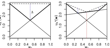
In order to select goodw’s for scalarization, OLS exploits the observation thatu∗X(w)is PWLC over the weight simplex. In particular, OLS selects only so-calledcorner weights that lie at the intersections of line segments of the PWLC functionu∗X(w)that correspond to the value vectors found so far. For example, in Figure 1 (left) there are two payoff vectors inX, and there is one corner weight. When OLS scalarizes the MO-CoG at this corner weight and solves it using a single-objective solver, it finds a new payoff vector, as shown in Figure 1 (right), improving it at the corner weight (as indicated by the red dashed line).
0.0 0.2 0.4 0.6 0.8 1.0
0.0
1.0
2.0
3.0
w1 uX
*
(
w
) Δ
0.0 0.2 0.4 0.6 0.8 1.0
0.0
1.0
2.0
3.0
w1 uX
*
(
w
[image:3.612.310.500.211.294.2])
Figure 1: (Left)The scalarized value as a func-tion of weightsu∗X(w)(bold segments) forX =
{(0,3),(3,0)}. There is one corner weight: (0.5,0.5). (Right) Adding a new payoff vector, (2.0,2.5), toX, thereby improvingu∗X(w). OLS prioritizes corner weights according to an
optimistic estimate of their potential error re-duction. The maximal potential error reduction that can be made by identifying a new payoff vectoru(a)is guaranteed to be at one of these corner weights [2]. In Figure 1, the potential er-ror reduction is denoted with dashed blue verti-cal lines. Note that the figure assumes that the single-objective solver is exact.
If this assumption holds, OLS is guaranteed to produce an exact CCS after solving a finite number of single-objective problems. If the single-objective solver returns a bounded ap-proximation instead, OLS inherits this quality bound.
Lemma 1. When an approximate single-objective solver produces a bounded approximate solution for each scalarized problem, with an error bound of at mostε, OLS produces anε-CCS [7].
2.3 Multi-Objective Coordination Graphs
Amulti-objective coordination graph(MO-CoG) [10] is a multi-objective decision problem that can be formally defined as a tuplehD,A,U iwhereD={1, ..., n}is the set ofnagents;A=A1×...×An is the set of all possible joint actionsa, the Cartesian product of the finite action spaces of all agents; andU =
u1, ...,uρ is the set ofρ,d-dimensionallocal payoff functions. A local payoff function has limited scopee, i.e., only a subset of agents participate in it. The total team payoff is the (vector) sum of all local payoffs:u(a) =P
ue∈Uue(ae). We refer to the set of all possible payoff vectors asV={u(a) :a∈ A}. For convenience, we assume thatVcontains both the values and associated joint actions. The additive functionu(a)can be expressed as a graphical model, i.e., a factor graph [1], where the agents are the vertices and the local payoff functions are the hyperedges connecting these vertices.
A MO-CoG can be linearly scalarized with a weight vectorw. Because of the additive nature of u(a), this scalarization distributes over the local payoff functions: uw(a) =Pue∈Uw·ue(ae). A scalarized MO-CoGis thus a single objective problem where the set of vector-valued local payoffs is replaced by a set of local payoff functions scalarized with a weightw:
Uw={ue
w(ae) =w·ue(ae) :ue(ae)∈ U }.
For convenience, we use justUwto refer to a scalarized MO-CoG asDandAare the same as in the MO-CoG. Because a scalarized MO-CoG is a single objective coordination graph, the maximal payoff can be determined with single-objective methods such as variable elimination, or, as we do in this paper, withvariational methods.
2.4 Variational Methods for Graphical Models
Variational techniques [12, 14] can be used to bound the maximal payoff of a single-objective co-ordination graph. The dual decomposition approach relaxes the combinatorial optimization into an easily evaluated bound, maxau(a) = maxaPue∈Uue(ae) ≤ Pue∈Umaxaeu
e(ae) = ¯u.
one finds a set of equivalent local payoffsu0e such that the total payoff is unchanged, u0(a) = maxaPu0e∈U0u0e(ae) = u(ae), while minimizing the decomposed upper bound. The resulting optimization is convex and can be solved using a number of gradient-based or fixed-point techniques [12]; our implementation uses a fixed-point update based onweighted mini-bucket[6].
The upper bound corresponds to an optimization of the individualue(a
e); if the optimal local actions a∗e are all consistent with somea∗, thena∗ is also the global optimum ofu(a). In practice, the decomposition bound may not be able to find the global optimum; for this reason, they typically also assemble a joint actionalusing, for example, greedy assignment. For each local payoffu0e(ae), we assign the elements ofaethat are not already assigned inalby maximizing the local function, conditioned on the already-assigned elements. The joint actionalthen provides a lower bound on the optimal payoff,u=u(al). We use this upper boundu¯, and the lower bound actional, to produce a bounded approximate CCS, in accordance with Lemma 1, in our new algorithm, described below.
3
Variational Optimistic Linear Support
In this section, we present our main contribution, variational optimistic linear support (VOLS). To our knowledge, VOLS is the first variational algorithm for solving MO-CoGs. Like previous OLS-based algorithms VOLS solves a MO-CoG as a series of single-objective coordination graphs. However, instead of relying on an exact single-objective solver, VOLS uses a variational method and can thus find approximate CCSs for much larger MO-CoGs than previous methods.
VOLS uses a variational subroutine for solving scalarized instances of the MO-CoG. This subroutine takes a scalarized MO-CoG as input. As output, the subroutine procudes a lower-bound joint action al, which we use to construct the approximate CCS. It also produces an upper bound u¯ on the optimal value, which we use to bound the quality of the final approximate CCS, and to prioritize instances in the series of single-objective problems to solve. Furthermore, the variational method manipulates the set of scalarized local payoff functionsUw to output a reparameterization, i.e., a set of manipulated local payoff functions U0
w for which all joint actions have the same (scalar)
payoff, i.e., ∀aP
ue∈U wu
e(a
e) = Pug∈U0 wu
g(a
g). A key insight is that we can re-use Uw0 to
hot-start the reparameterization of a new scalarized instance for a new weight vector zclose to w. Specifically, if we define thedifference graph between two scalarization weightsw andzas
Uw→z ={uew→z(ae) = (z−w)·ue(ae) :ue(ae)∈ U },then adding this difference graph to the reparameterizationU0
wyields a valid reparameterization forz,Uzˆ =Uw0 ∪ Uw→z. Whenwis close
toz, the magnitude of the local payoff functions inUw→zis small, andUzˆ is close toUw0 . Intuitively,
ˆ
Uzis therefore likely to be closer to the eventual reparameterizationU0
zthat the variational subroutine
will produce forUz, thanUzitself would be, and fewer iterations of the variational method will be required to further tighten the bounds and findU0
z.
The variational optimistic linear support (VOLS) algorithm (presented in Algorithm 1) takes a MO-CoG hD,A,U i and a variational single-objective coordination graph subroutine,
variationalSOSolver, as input. Following the OLS framework, VOLS keeps a setX, that will become an approximate CCS (line 1), and a set of upper bounds on the optimal values that VOLS finds for scalarized instances (for individualw),Uold(line 2). The algorithm starts looking for so-lutions (i.e., approximately optimal joint actions and payoffs) for the extrema of the weight simplex (line 3–4). VOLS keeps a setR(line 5) with tuples of weightswand reparameterizations produced at thosewbyvariationalSOSolverin iterations of the main loop.
In the main loop (lines 6–16), VOLS iteratively pops a corner weightw off the priority queueQ
and solves the corresponding scalarized MO-CoG,Uw. However, instead of just calling the single-objective solver forUwdirectly, VOLS first looks for the reparameterizationUv0 found in earlier
it-erations (on line 10), for the weight closest tow. Because∀a:P
ue∈U vu
e(a
e) =Pug∈U0 vu
g(a g), adding the difference graphUv→w ={uev→w(ae) = (w−v)·ue(ae) : ue(ae)∈ U }, results in a graphUˆw = Uv0 ∪ Uv→w, for which∀a Pue∈Uˆwue(ae) = Pug∈Uwug(ag). In other words, reusing the reparameterization forv on the scalarized graph forw does not affect the scalarized payoffuw(a)for anya.
Besides the reparameterizationU0
v∪ Uv→w,variationalSolveris also provided with the joint
actionavthat achieves the lower bound of the previous weightv. This joint action can be reused as
an initialguessfor the joint action atw. If at any time during the execution ofvariationalSolver
forU0
Algorithm 1:VOLS(hD,A,U i,variationalSOSolver)
Input: A MO-CoG
1 X← ∅; // approximate CCS of multi-objective payoff vectorsu(a) 2 Uold← ∅; // set of previouswanduw¯ , for determining optimistic estimates for new corner weights
3 Q←an empty priority queue ; // a priority queue with corner weights to search
4 Add extrema of the weight simplex toQwith infinite priority;
5 R ← ∅; // set of reparameterizations, joint actions, and associated weights
6 while¬Q.isEmpty()∧ ¬timeOutdo
7 w←Q.dequeue(); // retrieve a weight vector
8 Uv,0 av←select previous reparameterization and joint action found for the closest weightvtowfromR; 9 Uw,0 al, ¯uw←variationalSOSolver(U0
v∪ Uv→w); // a variational single objective solver.
10 R ← R ∪ {(w,Uw0,al)}; // store the reparameterization of the scalarized graph for reuse
11 Uold←Uold∪ {(w,uw)¯ }; // store upper bound forw, for determining the next max. possible improv.
12 ifu(al)6∈Xthen
13 X←X∪ {u(al)}; // add lower bound payoff and associated action,u(al), to the approximate CCS
14 W ←compute new corner weights and max. possible improvements(w,∆w)usingUoldandX;
15 Q.addAll(W);
16 end
17 end
18 returnX;
reuse, is thus highly effective when the variational single-objective solver can produce optimal solu-tions for the scalarized problem, as it can circumvent thedecodingphase of variational algorithms, which is often very computationally intensive.
The single-objective variational solver (called on line 9) produces three outputs: the new repa-rameterized graphU0
w, an upper bound on the optimal scalarized payoff,uw¯ , and the approximally
optimal joint actional. Note thatalimplies a lower bound on the optimal payoff inw, i.e.,w·u(al). All of these are stored (lines 10, 11 and 13).
Ifu(al)is not already inX, then it is added to it and new corner weights are identified. Then, VOLS calculates the maximal possible improvement for those corner weights by solving a linear program (line 14) [7, 10]. Finally, the new corner weights are added to the priority queueQ(line 15). Because the maximal possible improvement to the scalarized payoff is guaranteed to be at one of the corner weights ofX [2], VOLS terminates whenQis empty.
Upon termination, we can useUoldandXto determine the approximation qualityε, ofX using the following corollary of Lemma 1:
Corollary 1. VOLS returnsX, anε-CCS, where
ε= max
(w,¯uw)∈Uold
¯
uw−u∗X(w)
.
4
Experiments
In this section, we compare the performance of VELS and VOLS on randomly generated MO-CoGs. For the single-objective subroutine, we useweighted mini-buckets (WMB)[4, 6], with ani-bound ofi = 1. i = 1is the highest degree of approximation. The MO-CoGs are generated following the procedure of Roijers et al. [10], which can produce a MO-CoG for any specified number of:
nagents,dobjectives,ρlocal payoff functions, and|Ai|actions per agent. Starting from a fully connected graph withn(n−1)/2local payoff functions, each of which connects two random agents, local payoff functions are removed randomly, until onlyρremain. An edge is removed only if doing so does not cut the graph. Finally, each local payoff function is filled with vectors of lengthd, containing real numbers drawn independently and uniformly from[0,10].
We compare VELS and VOLS on random 3-objective MO-CoGs with increasing numbers of agents
Of course, VOLS produces only anε-CCS, whereas VELS produces an exact one. However, when we measureεusing Corollary 1, we find that it is consistently1.1%of the value or smaller. In fact, in Figure 2 (top right), it even appears to decrease as a function of the size of the problem. At 150 agents, VOLS (with reuse) produced anε-CCS with aεof only0.27%of the scalarized payoff. We thus conclude that VOLS’ improved scalability comes at only a negligible cost in terms of payoff.
To test the effect of reuse on runtime, we compare the runtime of VOLS with and without reuse. We ran both versions on the same 25 instances for each number of agents. Figure 2 (top left) shows that VOLS with reuse requires consistenly less runtime across all numbers of agents. Across all numbers of agents, VOLS with reuse is a factor1.22faster. Figure 2 (bottom left), shows the ratio of the runtimes of VOLS with and without reuse (the runtime with reuse divided by the runtime without reuse), and the ratio of theεproduced by VOLS with and without reuse. While the runtime ratio gradually increases, meaning less benefit from reuse, theεratio gradually increases, meaning better accuracy. Furthermore, VOLS with reuse has lower runtime and ε overall. Hence, reuse contributes positively to VOLS’ performance.
20 40 60 80 100 140
1e +0 2 1e +0 4 1e +0 6
number of agents
ru
nt
ime
(ms)
VELS VOLS no reuse VOLS with reuse
20 40 60 80 100 140
0.004
0.008
0.012
number of agents
ε (a s % o f sca l. pa yo
ff) VOLS with reuse
VOLS without reuse
20 40 60 80 100 140
0.70
0.80
0.90
1.00
number of agents
ra tio w ith /w ith ou t re use runtime ratio epsilon ratio
1e-08 1e-06 1e-04 1e-02 1e+00
1e -0 3 1e -0 1 1e +0 1 Δw ru nt ime ra tio
Figure 2: (Top left)The runtime (in logscale) of VOLS versus the runtime (in logscale) of VELS as a function of the number of agentsnwithρ= 1.8nandd= 3. The error bars represent SDOM.(Top right)The quality (ε) of the approximate CCSs produced by VOLS with and without reuse for the same MO-CoGs(Bottom left)The ratio of the runtimes andεof VOLS with and without reuse for the same MO-CoGs(Bottom right)The runtime of the variational subroutine for different weights with reuse, divided by the runtime without reuse in logscale, as a function of the difference with the closest weight∆w, for a MO-CoG withn= 125with
ρ= 1.8andd= 3.
We also tested the effect of reuse on the runtime of the single-objective subroutine inside VOLS, using
a single MO-CoG
withd = 3,n = 125 and ρ = 1.8n. For each weight w in the sequence, we exe-cuted the variational subroutine with and without reuse. The average total run-time with reuse was 0.10s while it was 0.16s without reuse. Figure 2 (bottom right) shows the ratio between the runtime with and without reuse as a function of ∆w=z−w, i.e., the distance between the current weight on the weight on which the reused reparameteri-zation is based. This figure shows that the runtime is positively correlated with ∆w. However, there are also a lot of weights
for which reuse has little or effect, and even a few outliers for which reuse has a negative effect on the runtime. These outliers contribute disproportionaly to the average runtime: although they make up only5%the weights, they are responsible for48%of the total runtime of VOLS with reuse. For comparison, the first5%of the calls, i.e., those with the5%largest∆w, account for only9%of the runtime. An interesting direction for future work is to develop a method for identifying these outliers before executing the single-objective subroutine and then employing reuse only when it is expected to help.
5
Conclusions
vari-ational method for MO-CoGs. VOLS solves a MO-CoG as a series of scalarized single-objective CoGs, for different scalarization weightsw. A key insight of VOLS is that the reparameteriza-tions outputted by variational methods for earlierwin the series can be reused when the variational single-objective subroutine is called again for a similar neww. Our experiments confirm that for large MO-CoGs, this reuse is key, and leads to both lower runtimes, and lower error. We therefore conclude that VOLS can efficiently solve large MO-CoGs that cannot be solved with exact methods, and that reparameterization reuse is a key component of the VOLS algorithm.
In future work, we aim to find a more efficient method, by analyzing and hopefully predicting the outliers of Figure 2 (bottom right). Furthermore, we aim to analyze the effect of thei-bound parameter of the WMB subroutine on the accuracy (in terms ofε) of VOLS.
Acknowledgments
This research is supported by NWO DTC-NCAP (#612.001.109) project, the NWO Innovational Research Incentives Scheme Veni (#639.021.336), and the NSF project #IIS-1254071. This work was carried out on the Dutch national e-infrastructure with the support of SURF Cooperative.
References
[1] C. M. Bishop. Pattern Recognition and Machine Learning. Springer, 2006.
[2] H.-T. Cheng. Algorithms for partially observable Markov decision processes. PhD thesis, University of British Columbia, Vancouver, 1988.
[3] C. Guestrin, D. Koller, and R. Parr. Multiagent planning with factored MDPs. InAdvances in Neural Information Processing Systems 15 (NIPS’02), 2002.
[4] A. T. Ihler, N. Flerova, R. Dechter, and L. Otten. Join-graph based cost-shifting schemes. In Proceedings of the Twenty-Eight Annual Conference on Uncertainty in Artificial Intelligence (UAI-12), pages 397–406, 2012.
[5] J. Kok and N. Vlassis. Collaborative multiagent reinforcement learning by payoff propagation. Journal of Machine Learning Research, 7:1789–1828, Dec. 2006.
[6] Q. Liu and A. T. Ihler. Bounding the partition function using H¨older’s inequality. In Proceed-ings of the 28th International Conference on Machine Learning (ICML-11), pages 849–856, 2011.
[7] D. M. Roijers, J. Scharpff, M. T. J. Spaan, F. A. Oliehoek, M. M. de Weerdt, and S. White-son. Bounded approximations for linear multi-objective planning under uncertainty. InICAPS 2014: Proceedings of the Twenty-Fourth International Conference on Automated Planning and Scheduling, pages 262–270, June 2014.
[8] D. M. Roijers, P. Vamplew, S. Whiteson, and R. Dazeley. A survey of multi-objective sequen-tial decision-making. Journal of Artificial Intelligence Research, 47:67–113, 2013.
[9] D. M. Roijers, S. Whiteson, and F. Oliehoek. Point-based planning for multi-objective POMDPs. InIJCAI 2015: Proceedings of the Twenty-Fourth International Joint Conference on Artificial Intelligence, pages 1666–1672, July 2015.
[10] D. M. Roijers, S. Whiteson, and F. A. Oliehoek. Computing convex coverage sets for faster multi-objective coordination.Journal of Artificial Intelligence Research, 52:399–443, 2015.
[11] A. Rosenthal. Nonserial dynamic programming is optimal. InProceedings of the Ninth Annual ACM Symposium on Theory of Computing, pages 98–105. ACM, 1977.
[12] D. Sontag, A. Globerson, and T. Jaakkola. Introduction to dual decomposition for inference. Optimization for Machine Learning, 1:219–254, 2011.
[13] P. Vamplew, R. Dazeley, E. Barker, and A. Kelarev. Constructing stochastic mixture policies for episodic multiobjective reinforcement learning tasks. InAdvances in Artificial Intelligence, pages 340–349. 2009.