promoting access to White Rose research papers
White Rose Research Online
[email protected]
Universities of Leeds, Sheffield and York
http://eprints.whiterose.ac.uk/
This is an author produced version of a paper published in
Physical Review A
.
White Rose Research Online URL for this paper:
Published paper
Zwierz, M., Perez-Delgado, C.A., Kok, P. (2010)
Unifying parameter estimation
and the Deutsch-Jozsa algorithm for continuous variables
, Physical Review A, 82
(4), Art no.042320
Marcin Zwierz,∗ Carlos A. Pérez-Delgado,† and Pieter Kok‡
Department of Physics and Astronomy, The University of Sheffield, Hounsfield Road, Sheffield, S3 7RH, United Kingdom
(Dated: November 9, 2010)
We reveal a close relationship between quantum metrology and the Deutsch-Jozsa algorithm on continuous variable quantum systems. We develop a general procedure, characterized by two parameters, that unifies pa-rameter estimation and the Deutsch-Jozsa algorithm. Depending on which papa-rameter we keep constant, the procedure implements either the parameter estimation protocol or the Deutsch-Jozsa algorithm. The parame-ter estimation part of the procedure attains the Heisenberg limit and is therefore optimal. Due to the use of approximate normalizable continuous variable eigenstates, the Deutsch-Jozsa algorithm is probabilistic. The procedure estimates a value of an unknown parameter and solves the Deutsch-Jozsa problem without the use of any entanglement.
PACS numbers: 03.67.Ac, 42.50.Ex, 06.20.-f
I. INTRODUCTION
Quantum metrology promises many advances in science and technology. Continuous variables (CV) are natural candidates for optical implementations of quantum metrology protocols [1–3]. The importance of continuous variables for quantum metrology stems from the unconditional and efficient charac-ter of CV preparation, manipulation and detection techniques [4,5]. In this paper, we devise an optimal parameter estima-tion procedure for continuous variables. Our procedure em-ploys a single continuous variable and estimates a value of an unknown parameter with Heisenberg-limited precision. Fur-thermore, for a particular, fixed value of the parameter in ques-tion the procedure behaves as the Deutsch-Jozsa algorithm for CVs. In fact our protocol extends the Deutsch-Jozsa algo-rithm over continuous variables presented by Pati and Braun-stein [6]. Instead of idealized, nonnormalizable and unphysi-cal states, we employ Gaussian states to represent continuous variables. Moreover, we define Gaussian states on a finite do-main, thus removing an unphysical, infinite speed-up over any classical procedure offered by the idealized states. An exten-sive analysis of the Deutsch-Jozsa algorithm over continuous variables was given by Adcock, Høyer, and Sanders [7].
The Deutsch-Jozsa algorithm is one of the first quantum algorithms, preceded only by the original Deutsch algorithm [8]. Even though the Deutsch-Jozsa problem is rather artifi-cial, the algorithm drew enormous attention due to the compu-tational speed-up over any classical procedure. The structure of the algorithm is simple enough to determine the source of this speed-up. The quantum superposition principle and con-sequent quantum parallelism that lie at the heart of quantum mechanics allows for the interference of many distinct compu-tational paths, and allows the correct answer to the problem to emerge in a single query. In other words, the Deutsch-Jozsa algorithm probes a global property of an unknown function
f(x)and returns the result in a single run.
∗Electronic address:[email protected]
†Electronic address:[email protected] ‡Electronic address:[email protected]
The paper is organized as follows. In Sec. II, we review the Deutsch-Jozsa algorithm over continuous variables and present its simplified version. In Sec. III, we review basic concepts in quantum metrology. In Sec.IV, we introduce a general procedure that unifies parameter estimation with the Deutsch-Jozsa algorithm, and we analyze it in detail. Finally, we make some concluding remarks in Sec.V.
II. DEUTSCH-JOZSA ALGORITHM OVER CONTINUOUS
VARIABLES
The generalization of the Deutsch-Jozsa algorithm to continu-ous variables was devised by Pati and Braunstein [6]. This generalization was implemented with idealized continuous variables defined on an infinite domain. However, we need to stress that any practical continuous-variable implementa-tion of the Deutsch-Jozsa problem can be realized only on a finite domain. Nevertheless, for simplicity, we first recall the Deutsch-Jozsa algorithm over continuous variables as origi-nally stated in Ref. [6].
The objective of the Deutsch-Jozsa problem is to determine whether some function f(x)is constant or balanced. This is achieved by Alice and Bob playing the following game. Al-ice submits a value ofxfrom−∞to+∞to Bob. Then Bob evaluates f(x), which can take only two values: 0 or 1. Bob also promises Alice to use either balanced or constant func-tions. A constant function is either 0 or 1 for all values of
x∈(−∞,+∞). A balanced function is 0 for half of the values of x, and 1 for the remaining values ofx. This is defined in terms of the Lebesgue measureµonR:µ(x∈R|f(x) =0) = µ(x∈R|f(x) =1)[6]. The goal of this game is the same as the objective of the Deutsch-Jozsa problem, i.e. to establish if the function used by Bob is constant or balanced. Classi-cally, Alice would have to submit infinitely many values ofx
to learn the global property of f(x)with certainty. However, if Bob can use a unitary black-box operation to calculate func-tion f(x), then a single function evaluation reveals the global property of f(x). In the setting of idealized continuous vari-ables, this would imply an infinite speed-up over any classical procedure.
2
|x0⟩ F
Uf
F−1
>= π
2 ⟩
[image:3.595.88.244.116.153.2]F
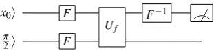
FIG. 1: A quantum circuit representing the Deutsch-Jozsa algorithm over continuous variables. The quantum networkNDJconsists of the Fourier transformsF and controlled black-box gateUf applied to the register and target CVs prepared in the idealized position eigen-states|x0⟩and|π/2⟩, respectively. The last operation is an inverse Fourier transform that enables the interference of different computa-tional paths.
algorithm over continuous variables shown in Fig.1. This implementation of the Deutsch-Jozsa algorithm employs two continuous variables, the so-called register and target CVs. Alice stores her query in the register CV, and the target CV is used by Bob during function evaluation. The register CV is prepared in the position eigenstate|x0⟩and the target in the
eigenstate|π/2⟩. The quantum network NDJ implementing
the Deutsch-Jozsa algorithm is given by the following unitary transformation
NDJ=Fr−1UfFrFt, (1)
whereFis the Fourier transform andr,tindicates the register and target CV, respectively. The Fourier transform applied to a CV in some position eigenstate|x⟩creates a superposition of all position eigenstates according to
F|x⟩=√1 π
∫ ∞
−∞dy e
2ixy|y⟩, (2)
where we used photon number units in which ¯h= 12. The unitary black-box operatorUf evaluates a value of function
f(x)and stores it in the state of the target CV:|x⟩|y⟩ −→ |x⟩|y+
f(x)⟩. Let us analyze the Deutsch-Jozsa algorithm step by step: (i) prepare the register and target CVs in an ideal position eigenstate|x0⟩and|π/2⟩, respectively; (ii) apply the Fourier
transformFto the register and target CVs
|s⟩=FrFt|x0⟩|π/2⟩=
1 π
∫ ∞
−∞dxdy e
2ixx0+iπy|x⟩|y⟩;
(iii) following the action of a unitary black-box operatorUf
the state of the CVs is given by
Uf|s⟩=
1
√ π
∫ ∞
−∞dx e
2ixx0e−iπf(x)|x⟩F t|π/2⟩;
(iv) the quantum network NDJ is finalized with an inverse
Fourier transformF−1applied to the register CV. Therefore, the state of the CVs can be written as
Fr−1Uf|s⟩=
1 π
∫ ∞
−∞dxdx
′e2ix(x0−x′)e−iπf(x)|x′⟩F t|π/2⟩;
(v) following the quantum networkNDJ, the property of
func-tion f(x)is determined by projecting the state of the register
CV onto the original position eigenstate|x0⟩. The
continuous-variable projection operator for idealized states can be written as
Px0=
∫ x0+ε
x0−ε
dy|y⟩⟨y|, (3)
whereε is the spread around x0 value, i.e. the
continuous-variable measurement cannot be performed with infinite pre-cision. The orthogonal complement ofPx0is given by
Px¯0=I−Px0=I−
∫ x0+ε
x0−ε
dy|y⟩⟨y|. (4)
By construction, a complete set of orthogonal projectors Pm
satisfy the completeness relation ∑mPm =I and PmPm′ =
δmm′Pm. If f(x)is constant then the measurement statistics
based on the above set of orthogonal projection operators and assumingε→0 is given by
p(x0) = Tr[Pˆx0ρDJ] =1, (5)
p(x¯0) = Tr[Pˆx¯0ρDJ] =0, (6)
wherep(x0)is the probability of measurement outcome to be
x0,p(x¯0)is the probability of a measurement outcome
differ-ent thanx0andρDJ=NDJ|r⟩|t⟩⟨t|⟨r|NDJ−1. Conversely, if f(x)
is balanced then the measurement statistics assumingε→0 is given by
p(x0) = Tr[Pˆx0ρDJ] =0, (7)
p(x¯0) = Tr[Pˆx¯0ρDJ] =1. (8)
Therefore, if the state of the register CV remains unchanged then the function f(x)is definitely constant, and if the state of the register CV is not|x0⟩ then the function f(x)is
bal-anced. A single function evaluation solves the Deutsch-Jozsa problem.
The core of the above implementation of the Deutsch-Jozsa algorithm is represented by a unitary, controlled black-box operator Uf applied between the Fourier transformed
reg-ister and target CVs. Here, the Fourier transformed target CV together with a black-box operator induces a phase shift, which depends on the global property of the function f(x):
Uf(|x⟩Ft|π/2⟩) = e−2i f(xˆ)pˆt|x⟩Ft|π/2⟩ =e−iπf(x)|x⟩Ft|π/2⟩.
Notice that the state of the target CV is not changed follow-ing the action ofUf. In factFt|π/2⟩is an eigenstate ofUf
with an eigenvaluee−iπf(x)“kicked back” in front of the regis-ter CV [9]. Conventionally, the Deutsch-Jozsa algorithm em-ploys multiple quantum systems, however, as the above sim-ple analysis of the action ofUf indicates the target CV can
be omitted. It is easy to show that a single register CV to-gether with a redefined black-box operatorUf≡e−2iπ/2f(xˆ)is
P
U
(
φ
)
Mp(x|φ)
ρ(0) ρ(φ)
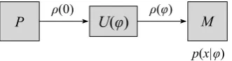
FIG. 2: The general parameter estimation procedure involving state preparationP, evolutionU(φ)and generalized measurementMwith outcomesx, which produces a probability distributionp(x|φ).
Moreover, the above implementation of the Deutsch-Jozsa al-gorithm is expressed in terms of the idealized position eigen-states. However, a more realistic and physically meaningful representation of a continuous variable is given by, for exam-ple, Gaussian states.
Similar to the setting of discrete quantum systems (e.g. qubits), some features of the Deutsch-Jozsa algorithm can serve as a starting point for developing other quantum al-gorithms. A slightly modified black-box operator Uf ≡
e−2iπ/2f(xˆ) for a simplified Deutsch-Jozsa algorithm can be used as the core of a protocol capable of estimating an un-known parameter that under appropriate conditions still re-tains the capabilities of the Deutsch-Jozsa algorithm. Before introducing this protocol, let us recall some basic concepts in quantum parameter estimation theory.
III. PARAMETER ESTIMATION
The most general parameter estimation procedure is shown in Fig.2, and consists of three elementary steps: (i) prepare a probe system in an initial quantum stateρ(0), (ii) evolve it to a stateρ(φ)by a unitary evolutionU(φ) =exp(−iφH), (iii) subject the probe system to a generalized measurement
M, described by a Positive Operator Valued Measure (POVM) that consists of elements ˆEx, where xdenotes the
measure-ment outcome. Here, the Hermitian operatorH is the gener-ator of translations inφ, the parameter we wish to estimate. The amount of information aboutφthat can be extracted by a measurement of the probe system is given by the Fisher infor-mation
F(φ) =
∑
x1
p(x|φ)
(
∂p(x|φ) ∂φ
)2
, (9)
where p(x|φ) =Tr[Eˆxρ(φ)] is the probability distribution
given by the Born rule that describes the measurement data, andxis a discrete measurement outcome. Based on the Fisher information one can bound a minimal value of the uncertainty inφwith the quantum Cramér-Rao bound [10–12]
(δφ)2≥ 1
T F(φ), (10)
where(δφ)2is the mean squared error in the parameterφ, and
T is the number of times the procedure is repeated. The ulti-mate limit of the quantum Cramér-Rao bound depends on how the Fisher information is bounded from above. The Fisher in-formation can be bounded in two ways: by the variance ofH
|G(x0)⟩ F Uf(φ) F−1
[image:4.595.89.255.108.152.2]>=
FIG. 3: A quantum circuit representing the general protocol over continuous variables. The quantum network consists of the Fourier transformF and black-box gateUf(φ)applied to a single register CV prepared in the Gaussian state|G(x0)⟩. The last operation is an inverse Fourier transformation that enables the interference of differ-ent computational paths.
[13] or by the expectation value ofH [14,15]
F(φ)≤16(∆H)2 and F(φ)≤4⟨H⟩2, (11) where we again used ¯h=12. Since both bounds are completely general and complement each other, any parameter estimation procedure must respect them. Typically, the Fisher informa-tion is related to an appropriate resource count such as the average photon number, the average energy of the probe sys-tem or the number of unitary evolution gates that are used in the estimation procedure. The expectation value ofH plays the role of the resource count [14]. We usually consider two scaling regimes of the quantum Cramér-Rao bound. The first regime: the so-called standard quantum limit(SQL) [16] or
shot-noise limitis obtained when the Fisher information is a constant with respect toT and the resource count. TheSQLis typically given by
δφ&√1
T . (12)
The second regime: the so-calledHeisenberg limit[17] is ob-tained in a single-shot experiment (T =1) when the Fisher information scales quadratically with the resource count. The Heisenberg limit is then given by
δφ≥√1
F(φ). (13)
Therefore, the uncertainty in the parameterφ scales linearly inversely with the resource count. Both scaling regimes of the quantum Cramér-Rao bound can be compared directly in terms of an appropriate resource count [14].
IV. GENERAL PROCEDURE WITH GAUSSIAN STATES
In this section, we present a general procedure capable of de-termining the value of a single parameterφ∈[0,2π)or im-plementing the Deutsch-Jozsa algorithm (see Fig. 3). Here, the black-box operator is defined in the following way
Uf(φ)≡exp(−2iφf(xˆ)), (14)
4
algorithm, any physical continuous-variables parameter esti-mation protocol can be implemented only on a finite domain. Therefore, we introduce the semi-Gaussian input state defined on a finite domain given by
|G(x0)⟩=
∫ T −T dx Nx exp [
−(x−x0)2
2∆2
]
|x⟩, (15)
where∆is the variance of the state andNxis the normalization
constant given by Nx2 =√π∆2/2[erf(T+x0
∆ ) +erf(T−∆x0)
] .
We note that for∆≪T we recover the normalization con-stant in the form ofNx2=√π∆2which is characteristic for a
Gaussian state defined on an infinite domain, i.e. from−∞to
+∞. The Fourier transformed semi-Gaussian state defined on a finite domain can be written as
|G(p0)⟩=
∫ P
−P
d p Np
exp[−2∆2(p−p0)2
]
|p⟩, (16)
where 1/(2∆)is the variance of the Fourier transformed semi-Gaussian state andNpis given by
N2p=
√ π/4∆2
2 [erf(2(P+p0)∆) +erf(2(P−p0)∆)]. ForP≫1/(2∆) the normalization constant takes the form of N2p=√π/4∆2, characteristic for a Fourier transformed
Gaussian state define on an infinite domain. The relation-ship between domains of the semi-Gaussian input state and its Fourier transformed counterpart is given byP=1/(2T).
The general procedure consists of the following instruc-tions: (i) prepare the register CV in the normalized semi-Gaussian state|r⟩=|G(x0)⟩, and apply the Fourier transform
Fdefined by
F|x⟩=|x⟩p=
1
√
2T
∫ T
−T
dy e2ixy|y⟩, (17)
where|x⟩pis the Fourier transformed position eigenstate, i.e.
the momentum eigenstate; (ii) subsequently, a black-box op-eratorUf(φ)is applied. Then the state of the system is
Uf(φ)F|r⟩ =
∫ T −T dx Nx exp [
−(x−x0)2
2∆2
]
e−2iφf(xˆ)|x⟩p
= √1
2T ∫ T −T dxdy Nx exp [
−(x−x0)2
2∆2
]
×e2iyxe−2iφf(y)|y⟩;
(iii) finally, an inverse Fourier transformF−1is applied fol-lowed by a measurement. The state of the register CV is mea-sured by projecting onto the original semi-Gaussian state cen-tered aroundx0. Measurement is described by a POVM set
{Px0,Px¯0}, where
Px0=
∫ T
−T
dxdy gxy|x⟩⟨y|,andPx¯0 =I−Px0 (18)
with
gxy=
1
N2
ε exp
[
−(x−x0)2
2ε2
] exp
[
−(y−x0)2
2ε2
]
, (19)
andεis the intrinsic precision of the measurement apparatus, i.e. any continuous-variable measurement must have finite precision if it is to be physical, andNε is the normalization constant given by Nε2 = √πε2/2[erf(T+x0
ε ) +erf(T−εx0)
] .
The optimal measurement which corresponds to the initial semi-Gaussian register state hasε=∆, thusNε=Nx.
Now let us calculate the measurement statistics. Analyti-cal expressions for the measurement statistics are hard to find due to the presence of error functions erf(x). However, for the semi-Gaussian states with∆≪Tthe calculations simplify considerably. Under this regime, the limits of integration for the integrals containing terms that depend on∆ range from
−∞to+∞. Necessarily, the normalization constants have to be changed and are expressed as√2T Nx=
√ π√4
π∆2. In other
words, a semi-Gaussian input state defined on a finite domain is approximated with a Gaussian state defined on an infinite domain. Therefore, the measurement statistics based on the above POVM are given by the following expression
p(x0|φ) =
4∆2 π
∫ P
−P
dzdy e−4∆2(z2+y2)e2iφ(f(z)−f(y)),
p(x¯0|φ) = 1−p(x0|φ). (20)
Here, the interval (−P,P) is a finite domain of the Fourier transformed semi-Gaussian state|G(x0)⟩, and denotes the
in-terval, where for this particular procedure function f(x)is de-fined.
At this point, we have to give an explicit definition of the function. Functions f(x) defined on a finite domain return-ing only two values({0,1})fall into three distinct categories: constant, balanced and neither constant nor balanced. We re-call that the objective of the Deutsch-Jozsa algorithm is to probe whether an unknown function f(x)is constant or bal-anced. We parameterize the three possibilities for defining
f(x)by introducing a parameterr. The above integrals can then be evaluated for any function f(x) behaving as a step function, with the parameterrmarking the point where f(x)
changes its value. Hence, forr=0 andr=±Pthe function
f(x) is balanced and constant, respectively. For 0<r<P
(or −P<r<0), the function f(x)is neither constant nor balanced. We consider only positive values of rdue to the symmetry of the setup. This leads to
p(x0|φ) =
1 2 [
erf2(2P∆) +erf2(2r∆)]+
1 2 [
erf2(2P∆)−erf2(2r∆)]cos(2φ),
p(x¯0|φ) = 1−p(x0|φ),
wherep(x0|φ)is the probability of measurement outcome to
be in the intervalx0±εandp(x¯0|φ)is the probability of
A. Representations off(x)
Our choice to represent f(x)as a step function simplified our calculations. However, we can imagine more elaborate be-havior patterns for f(x). In principle, since in the case of the Fourier transformed idealized continuous variables all terms have amplitudes of equal magnitude, all finite sub-intervals, where the function takes value 0 can be added up to a single interval. The same applies to all sub-intervals, where function takes value 1. Therefore, one ends up with two intervals and a relationship between them given by the parameterr. However, in the setting of semi-Gaussian states defined on a finite do-main, the above reasoning is not quite as straightforward. The amplitudes of the Fourier transformed Gaussian states have a slightly different magnitude. One may notice this feature by inspecting Eq. (20). Since in our calculations we favor a step-function representation over any other, let us estimate the maximum error we make with this assumption. Due to a triv-ial nature of a constant function, in the following analysis we consider a balanced function. We consider the step-function representation of a balanced function withr=0. The biggest deviation from this representation is offered by a balanced function that changes its value twice at pointsr1=−P/2 and
r2=P/2. Both representations produce two distinct
probabil-ity distributionspstep(x0|φ)andphat(x0|φ), respectively, that
differ by the errorεP∆given by
εP∆=|1−cos(2φ)| ×
−8
π(P∆)6+ 24
π (P∆)8+O (
(P∆)10).
The error tends to zero withP∆→0. This is natural since when ∆→0 all amplitudes of the Fourier transformed ide-alized position eigenstate have the same magnitude, i.e., the spectrum is flat.
B. Analysis
Our procedure can be analyzed in two ways. As expected, from one perspective it behaves as a parameter estimation pro-tocol. From the other, it behaves as the Deutsch-Jozsa algo-rithm. First, we analyze the behavior of the parameter estima-tion part of the procedure. Based on the above measurement statistics, we calculate the Fisher informationF(φ). The min-imal value ofF(φ) =0 occurs when function f(x)is constant (r=P) with the corresponding measurement statistics
p(x0|φ) = erf2(2P∆),
p(x¯0|φ) = 1−erf2(2P∆).
Conversely, the maximal value of the Fisher information
F(φ) = 4 erf
2(2P∆)(cos(2φ)−1)
erf2(2P∆)(cos(2φ) +1)−2 (21)
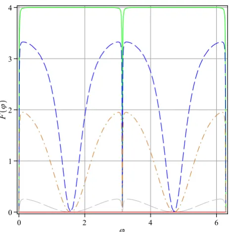
FIG. 4: (Color online) General dependence of the Fisher informa-tionF(φ)for five values of the parameterr: r=0 corresponds to the uppermost solid line (green),r=P/8 corresponds to the dashed line (blue),r=P/4 corresponds to the dashed-dotted line (brown),
r=P/2 corresponds to the long dashed line (gray), andr=P corre-sponds to the lowermost solid line (red).
occurs when function f(x)is balanced (r=0) with the corre-sponding measurement statistics
p(x0|φ) =
1 2erf
2(2P∆) [1+cos(2φ)],
p(x¯0|φ) = 1−
1 2erf
2(2P∆) [1+cos(2φ)].
Here, the optimal value of the Fisher informationF(φ) =4 is given for erf2(2P∆) =1⇒P≥3/(2∆)which, in general, impliesP&1/(2∆)and is consistent with the approximation applied above. The general dependence of the Fisher informa-tionF(φ)on parameterrwithP=3/(2∆)and∆=1/√2 (the variance of the coherent state) is shown in Fig.4. The dips that are especially visible for the balanced function appear because the Fisher informationF(φ)retains some dependence on the parameterφ since forP=3/(2∆): erf2(2P∆)≈1. Based on the general dependence of F(φ)onr, we conclude that the maximal value of the Fisher information is indeed obtained for a balanced function.
To address the optimality of our parameter estimation pro-tocol, we analyze the behavior of the generator of translations in the parameterφ:H ≡f(xˆ). The expectation value of the generatorH in the state of the register CV preceding applica-tion of the black-box operator, i.e. |ψin⟩=F|r⟩with∆≪T,
is given by
⟨H⟩=⟨f(xˆ)⟩=1
2(erf(2P∆)−erf(2r∆)).
[image:6.595.323.556.109.344.2]6
can be written as
(∆H)2= (∆f(xˆ))2 = 1
2(erf(2P∆)−erf(2r∆))× [
1−1
2(erf(2P∆)−erf(2r∆)) ]
.
The maximal expectation value of the generatorH occurs for a balanced function (r=0) withP≥3/(2∆)and is given by
⟨H⟩=1/2. On the other hand, the maximal variance of the generatorH is(∆H)2=1/4. Hence, the Fisher information is bounded byF(φ)≤16(∆H)2=4. Therefore, we note that according to Eqs. (11) and (13) our procedure attains the scaling regime of the Heisenberg limit. However to establish its optimality we must calculate whetherδφ=1/√F(φ). We use the standard expression for the mean squared error given by
δφ= ∆X
|d⟨X⟩/dφ|, (22)
where X is the measurement observable defined as X =
Px0 [see Eq. (18)]. Hence, for the final state ψφ
⟩
=
F−1Uf(φ)F|r⟩withε=∆we calculate⟨X⟩=⟨ψφ|Px0|ψφ⟩=
1 2erf
2(2P∆) [1+cos(2φ)]. Based on the propertyP2
x0=Px0we
find that⟨X2⟩=⟨X⟩. ForP≥3/(2∆)the mean squared error isδφ=1/2. Hence, we conclude that for a balanced function our parameter estimation procedure over continuous variables attains the ultimate limit of the quantum Cramér-Rao bound, and therefore is optimal. This result constitutes an analogy to the phase estimation with a qubit realized as a single photon placed in the arms of the Mach-Zender interferometer. Here, the balanced property of function f(x)plays a role of two dis-tinct paths in a balanced Mach-Zender interferometer.
Next, let us analyze the Deutsch-Jozsa side of the proce-dure. Under appropriate conditions the developed procedure can determine the character of function f(x). If a value of the parameterφis fixed:φ=π/2 then the measurement statistics is given by
p(x0) = erf2(2r∆),
p(x¯0) = 1−erf2(2r∆),
It is clear that for a constant and balanced function f(x)the corresponding measurement statistics of the Deutsch-Jozsa al-gorithm are recovered. Indeed, when functionf(x)is constant (r=P) then
p(x0) = erf2(2P∆),
p(x¯0) = 1−erf2(2P∆),
and when function f(x)is balanced (r=0) then p(x0) =0
andp(x¯0) =1. The Deutsch-Jozsa algorithm over the
semi-Gaussian states defined on a finite domain becomes a prob-abilistic procedure. This is consistent with the conclusions found in Ref. [7]. However, when the size of the domain is sufficiently large withP≥3/(2∆)then a definite distinction between constant and balanced functions can be made. Never-theless, even for large enough domains this implementation of
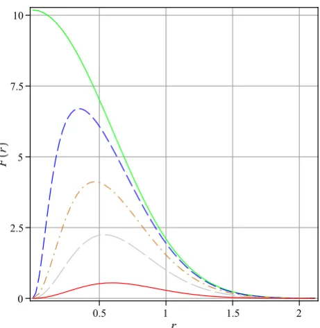
FIG. 5: (Color online) General dependence of the Fisher information
F(r)for four values of the parameterφ:φ=π/2 corresponds to the uppermost solid line (green),φ=5π/12 corresponds to the dashed line (blue),φ=π/3 corresponds to the dashed-dotted line (brown),
φ=π/4 corresponds to the long dashed line (gray), andφ=π/8 corresponds to the lowermost solid line (red). The optimal value ofr
shifts from balanced to constant.
the Deutsch-Jozsa protocol does not offer an unphysical, infi-nite speed-up over the classical procedures. We note that for ideal, nonnormalizable position eigenstates (∆→0), the con-stant function measurement statistics is retained forP→∞
renderingPandrunphysical, thus making a meaningful dis-tinction between the balanced and constant functions impos-sible.
We also calculated the Fisher information F(r) and plot-ted it againstr∈(0,P)for five different values of the param-eter φ={π/2,5π/12,π/3,π/4,π/8} withP=3/(2∆)and
∆=1/√2 (see Fig.5). The maximal value of the Fisher infor-mationF(r)is obtained forφ=π/2 corresponding to a sim-plified Deutsch-Jozsa algorithm. We note that the optimality changes from balanced to more constant whenφ̸=π/2. Any further analysis of this side of the procedure is problematic due to a lack of the generator of translations inr.
[image:7.595.324.555.107.344.2]continuous variables.
V. CONCLUSIONS
In conclusion, we developed a general procedure capable of performing two distinct tasks. For one mode of operation the protocol estimates a value of an unknown parameter with Heisenberg-limited precision. On the other hand, for a fixed value of the parameter in question the procedure addresses the Deutsch-Jozsa problem in a single run. Our procedure em-ploys Fourier transforms and black-box unitary operator ap-plied to a single continuous variable represented as the semi-Gaussian state defined on a finite domain. Consequently, for this setup, the parameter estimation side of the proce-dure is optimal and the Deutsch-Jozsa algorithm offers finite,
i.e. physically feasible, speed-up over any classical proce-dure. Furthermore, no entanglement is present at any stage of the procedure. A similar conclusions concerning quan-tum metrology can be found in Refs. [18,19]. We emphasize a special role played by balanced functions f(x). The pro-cedure equipped with the black-box operator that introduces the parameterφvia the balanced function attains the ultimate limit of the quantum Cramér-Rao bound. This behavior can be linked to the phase estimation with a qubit realized as a single photon placed in the arms of the Mach-Zender interferometer.
Acknowledgments
This work was supported by the White Rose Foundation and the QIPIRC programme of the EPSRC.
[1] C. M. Caves. Quantum-mechanical noise in an interferometer.
Phys. Rev. D, 23:1693, 1981.
[2] S. L. Braunstein and H. J. Kimble. Teleportation of continuous quantum variables.Phys. Rev. Lett., 80:869, 1998.
[3] P. Kok and B. W. Lovett. Introduction to Optical Quantum In-formation Processing. Cambridge University Press, 2010. [4] S. L. Braunstein and P. van Loock. Quantum information with
continuous variables.Rev. Mod. Phys., 77:513, 2005.
[5] S. Lloyd and S. L. Braunstein. Quantum computation over con-tinuous variables.Phys. Rev. Lett., 82:1784, 1999.
[6] A. K. Pati and S. L. Braunstein. Deutsch-Jozsa algorithm for continuous variables. InQuantum Information with Continuous Variables. Kluwer Academic Publisher, 2003.
[7] M. R. A. Adcock, P. Høyer, and B. C. Sanders. Limitations on continuous variable quantum algorithms with Fourier trans-forms.New J. Phys., 11:103035, 2009.
[8] D. Deutsch and R. Jozsa. Rapid solution of problems by quan-tum computation. InProceedings of the Royal Society of Lon-don, volume A439, pages 553–558, 1992.
[9] R. Cleve, A. Ekert, C. Macchiavello and M. Mosca. Quan-tum algorithms revisited. In Proceedings of the Royal Soci-ety of London, volume A454, pages 339–354, 1998. e-print arXiv:quant-ph/9708016.
[10] C. W. Helstrom. Minimum mean-squared error of estimates in quantum statistics.Phys. Letters, 25A:101–102, 1967.
[11] C. W. Helstrom. Quantum detection and estimation theory.
Journal of Statistical Physics, 1:231–252, 1969.
[12] S. L. Braunstein and C. M. Caves. Statistical distance and the geometry of quantum states. Phys. Rev. Lett., 72:3439–3443, 1994.
[13] S. L. Braunstein, C. M. Caves, and G. J. Milburn. General-ized uncertainty relations: Theory, examples, and Lorentz in-variance.Ann. Phys., 247:135–173, 1996.
[14] M. Zwierz, C. A. Pérez-Delgado, and P. Kok. General optimal-ity of the Heisenberg limit for quantum metrology. Phys. Rev. Lett., 105:180402, 2010.
[15] P. J. Jones and P. Kok. Geometric derivation of the quantum speed limit.Phys. Rev. A, 82:022107, 2010.
[16] C. W. Gardiner and P. Zoller.Quantum Noise. Springer-Verlag, 3rd edition, 2010.
[17] M. J. Holland and K. Burnett. Interferometric detection of optical phase shifts at the Heisenberg limit. Phys. Rev. Lett., 71:1355–1358, 1993.
[18] T. Tilma, S. Hamaji, W. J. Munro, and K. Nemoto. Entangle-ment is not a critical resource for quantum metrology. Phys. Rev. A, 81:022108, 2010.