What is the orientation of the tip in a scanning tunneling microscope?

arXiv:1501.06538v1 [cond-mat.mtrl-sci] 26 Jan 2015

What is the orientation of the tip in a scanning tunneling

microscope?

G´abor M´andi

Department of Theoretical Physics, Budapest University of Technology and Economics,

Budafoki ´ut 8., H-1111 Budapest, Hungary

Gilberto Teobaldi

Stephenson Institute for Renewable Energy and Surface Science Research Centre,

Department of Chemistry, University of Liverpool,

L69 3BX Liverpool, United Kingdom

Kriszti´an Palot´as∗

Department of Theoretical Physics,

Budapest University of Technology and Economics,

Budafoki ´ut 8., H-1111 Budapest, Hungary

Abstract

The atomic structure and electronic properties of the tip apex can strongly affect the contrast

of scanning tunneling microscopy (STM) images. This is a critical issue in STM imaging

given the, to date unsolved, experimental limitations in precise control of the tip apex atomic

structure. Definition of statistically robust procedures to indirectly obtain information on the

tip apex structure is highly desirable as it would open up for more rigorous interpretation and

comparison of STM images from different experiments. To this end, here we introduce a statistical

correlation analysis method to obtain information on the local geometry and orientation of the

tip used in STM experiments based on large scale simulations. The key quantity is the relative

brightness correlation of constant-current topographs between experimental and simulated data.

This correlation can be analyzed statistically for a large number of modeled tip orientations and

geometries. Assuming a stable tip during the STM scans and based on the correlation distribution,

it is possible to determine the tip orientations that are most likely present in an STM experiment,

and exclude other orientations. This is especially important for substrates such as highly oriented

pyrolytic graphite (HOPG) since its STM contrast is strongly tip dependent, which makes

interpretation and comparison of STM images very challenging. We illustrate the applicability

of our method considering the HOPG surface in combination with tungsten tip models of two

different apex geometries and 18144 different orientations. We calculate constant-current profiles

along the h1100i direction of the HOPG(0001) surface in the |V| ≤1 V bias voltage range, and

compare them with experimental data. We find that a blunt tip model provides better correlation

with the experiment for a wider range of tip orientations and bias voltages than a sharp tip model.

Such a combination of experiments and large scale simulations opens up the way for obtaining

more detailed information on the structure of the tip apex and more reliable interpretation of

STM data in the view of local tip geometry effects.

Keywords: STM, tip geometry, tip orientation, correlation, statistical analysis, graphite, HOPG

I. INTRODUCTION

The interpretation of scanning tunneling microscopy (STM) images is not straightforward due to the effects of the local tip apex geometry, termination and orientation. The reason is the convolution of sample and tip electronic states in a given energy window defined by the

bias voltage, and the fact that in STM experiments the detailed atomic geometry around the tip apex is practically unknown and hardly controllable. On the other hand, it is clear

that the electronic states and their dominating orbital characters involved in the tunneling depend very much on the local atomic structure of the tip apex.

It has been a challenge to obtain information about the relevant properties of the STM tip apex for a long time. Herz et al. performed reverse STM imaging experiments to study

p,d, andf orbital characters of the tip apex atom above the Si(111)-(7×7) surface [1]. The combination of STM experiments and simulations on well characterized surfaces to obtain

information on the tip structure and termination was used, e.g., by Chaikaet al. [2, 3]. They considered the highly oriented pyrolytic graphite (HOPG) surface in the (0001) crystallo-graphic orientation in combination with W(001) tip models. Rodary et al. studied Cr/W

tip apex structures by high resolution transmission electron microscopy, and they pointed out that the magnetization direction of monocrystalline nanotips cannot be controlled in spin-polarized STM [4]. Recently, the effect of the tip orbitals on the STM imaging of

supported molecular structures attracted considerable attention. Gross et al. investigated pentacene and naphthalocyanine molecules on NaCl/Cu(111) surface by CO-functionalized

tips, and they explained the obtained STM contrast by tunneling through the p-states of the CO molecule [5]. Siegert et al. developed a reduced density matrix formalism in com-bination with Chen’s derivative rule [6] to describe electron transport in STM junctions for

molecular quantum dots, and studied the effect of selected tip orbital symmetries on the STM images of the hydrogen phthalocyanine molecule on a thin insulating film [7]. Lakin

et al. proposed a method to deconvolute STM images and determine molecular orientations of both the sample and the functionalized tip [8]. In their work a C60-Si(111)-(7×7) surface

and a C60-functionalized tip were chosen.

Even in seemingly less complicated STM junctions, only a few theoretical works focused

on the effect of the tip orientation on the STM images. Hagelaar et al. demonstrated that a wide range of modeled tip terminations and orientations can reproduce the experimental

images for NO adsorbed on Rh(111) [9]. This work also showed that the modeling of realistic

tip structures, including nonsymmetric tips, is desirable for a good qualitative reproduction of experimental STM images. However, it is quite unlikely that the relative orientation of

the sample surface and the local tip apex geometry in STM experiments is of high symmetry, which has been commonly assumed in the vast majority of STM simulations to date. M´andi

et al. studied the effect of asymmetric relative tip-sample orientations on the STM contrast of the W(110) metal surface [10] and of the HOPG(0001) surface [11] employing a three-dimensional Wentzel-Kramers-Brillouin (3D-WKB) electron tunneling theory. It was found

that the STM images can be substantially distorted due to tip geometry effects. A physical explanation was provided based on the real-space shape of the electron orbitals entering the orbital-dependent tunneling transmission formula in the 3D-WKB method [10], see Eq.(A8)

in Appendix. Motivated by the ideas of Hagelaar et al. and based on the methodology of M´andi et al., in the present work a new concept of obtaining information about the

local spatial orientation of the STM tip in real instruments is introduced. The concept is substantiated by a combination of STM experiments and large scale simulations taking the HOPG(0001) surface. Concomitantly, the qualitative visual analysis of STM images is

advanced by quantifying their correspondence in terms of relative brightness correlations.

The paper is organized as follows: The proposed correlation analysis method is introduced in section II, followed by its application to the HOPG(0001) surface. We analyze and discuss our results in section III, and summarize our findings in section IV. The appendix reports a

brief summary of the 3D-WKB tunneling theory with an arbitrary tip orientation.

II. METHOD

To quantitatively compare the experimental (EXP) and simulated (SIM) constant-current

topographs, the definition of the relative brightness of a given two-dimensional (2D) contour

C at bias voltage Vk is needed [11, 12]:

BC(x, Vk) =

zC(x, Vk)−zC(xmin, Vk)

zC(xmax, Vk)−zC(xmin, Vk)

, (1)

where zC(x, Vk) is the apparent height of the constant-current contour C above the surface

lateral x = xij position at bias voltage Vk obtained by C ∈ {EXP,SIM}. zC(xmin, Vk)

area, thus due to the definition, BC(xmin, Vk) = 0 andBC(xmax, Vk) = 1. Assuming that all

BC(xij, Vk) contours consist of Nx×Ny points (i= 1, ..., Nx, j = 1, ..., Ny), the mean value

of the relative brightness in a given bias voltage range ofNV bias values (k = 1, ..., NV) can

be calculated as

BC =

1

NxNyNV

NV X k=1 Nx X i=1 Ny X j=1

BC(xij, Vk). (2)

Using the same resolution of the scanning area in the experiment and in the simulations resulting in relative brightness contours ofNx×Ny lateral points in both cases, it is possible

to quantitatively compare the BEXP and BSIM contours in the corresponding bias voltage

range of NV bias values by calculating their correlation coefficient as

r =    NV X k=1 Nx X i=1 Ny X j=1

[BEXP(xij, Vk)−BEXP][BSIM(xij, Vk)−BSIM]    ×    NV X k=1 Nx X i=1 Ny X j=1

[BEXP(xij, Vk)−BEXP]2 





−1/2

×    NV X k=1 Nx X i=1 Ny X j=1

[BSIM(xij, Vk)−BSIM]2 





−1/2

. (3)

The (Pearson product-moment) correlation coefficient r measures the degree of linear rela-tionship between the BEXP(xij, Vk) and BSIM(xij, Vk) datasets. Due to the definition, the

values of r are bounded to the range of [-1, +1]. r = +1 corresponds to a perfect positive linear relationship that is desirable when comparing relative brightness contours between experiment and simulations. Obtaining r = +1 would mean that the simulation

repro-duces the experimental data perfectly. r =−1 means a perfect negative linear relationship, e.g., this would be the result of calculating the correlation coefficient of exactly oppositely

corrugated contours. r= 0 means that there is no linear relationship between the contours. Another statistical measure for the difference between experimental and simulated con-tours is the mean squared error,

MSE=_N 1

xNyNV

PNV

k=1

PNx

i=1P

Ny

j=1[BEXP(xij, Vk)−BSIM(xij, Vk)]2.

A perfect agreement of contours is obtained at MSE=0, and it is desired that MSE is

mini-mal comparing experimental and simulated contours for obtaining the best agreement. For selected contours and bias voltages we found good correspondence between minimal MSE and maximal correlation. However, MSE is not bounded from above, and this makes the

analysis of MSE distribution and the interpretation of maximal MSE difficult. Therefore, we excluded using this measure in our statistical analysis.

The calculation of the correlation coefficient in Eq.(3) was presented in the more general

case of taking 2D relative brightness contours. However, the same method can be specifi-cally applied to one-dimensional (1D) relative brightness profiles by setting Ny = 1. This

approach will be used in the paper for the h1¯100i direction of the HOPG(0001) surface since experimental data [12] is available for such a case. To calculate the relative bright-ness correlations between the experiment and simulations, profiles shifted to start with their

minimum value, BC(xi=1,j=1, Vk) = 0 are taken. A detailed discussion justifying this was

given in section 3.2. of Ref. [11].

Since in the simulations the tip material (TIPMAT), atomic arrangement/geometry (TIP-GEO), and orientation described by the Euler angles (θ0, φ0, ψ0) can be chosen in practically

infinite ways, the corresponding relative brightness profiles are dependent on these parame-ters:

BSIM(x, Vk) =BSIM(x, Vk,TIPMATTIPGEO, θ0, φ0, ψ0), and similarly, the correlation

coeffi-cient is r = r(TIPMATTIPGEO, θ0, φ0, ψ0). In the present work, we consider TIPMAT=W

(tungsten) and TIPGEO ∈ {blunt,sharp} tip models. The Wblunt tip is represented by an

adatom adsorbed on the hollow site of the W(110) surface and the Wsharp tip is modeled

as a pyramid of three-atoms height on the W(110) surface. More details on the used tip geometries can be found in Ref. [12]. These tip models are expected to bracket the range of

possible tip sharpnesses in experiments as extremely blunt tips with flat surfaces would pro-vide no contrast-resolution at all and sharp pyramids would likely be very unstable during prolonged tip scans. Moreover, carbon-contaminated tips with a C atom at the apex can be

excluded due to a dramatic decrease of the tunneling current [12].

In our simulations the three-dimensional Wentzel-Kramers-Brillouin (3D-WKB) electron

tunneling theory with arbitrary tip orientations is employed, see Appendix, which is imple-mented in the 3D-WKB-STM code [10, 13, 14]. Recently, the 3D-WKB method was

suc-cessfully applied in a number of theoretical [15–19] and combined experimental-theoretical investigations [20].

Constant-current brightness profiles are calculated along the h1¯100i direction (x-axis of Fig. 1) containing the three characteristic positions of the HOPG(0001) surface: hollow (h),

α-carbon and β-carbon, see inset of Fig. 1. The experimental averaged brightness data with

Ny = 1 and Nx = 46 points are taken from Fig. 4 of Ref. [12] in the interval of [-1 V, 1 V]

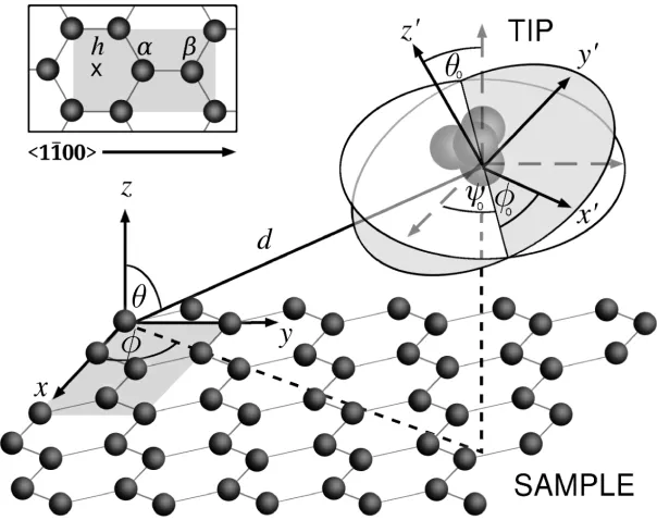
FIG. 1: Schematic view of the STM tip above the HOPG surface. The rotation of the local coordinate system of the tip with respect to that of the sample surface is described

by the Euler angles (θ0, φ0, ψ0). Inset shows the positions of the characteristic h, α and β

sites of the HOPG(0001) surface along the h1¯100idirection.

bias voltage in such a way that the lowest apparent height of each constant-current contour is zSIM(xmin, Vk) = 5.5 ˚A (pure tunneling regime). The relative brightness profiles are

calculated by using the introduced Wblunt and Wsharp tip models for a set of tip orientations

described by the Euler angles: θ0 ∈ [0◦,30◦], φ0 ∈ [0◦,175◦], ψ0 ∈ [0◦,355◦] with 5◦ steps.

The Euler angles are visualized in Fig. 1. θ0 angle describes the rotation with respect to the

x axis, transforming the z axis to z′_{. Additionally, φ}

0 and ψ0 are rotation angles around

the z′ _{and z axes, respectively, as Fig. 1 shows. The exact meaning of the Euler angles is} mathematically formulated in the rotation matrix in Eq.(A11) in Appendix and explained

in Refs. [10, 11]. Altogether 7 ×36× 72 = 18144 tip orientations are considered. For this selection we used the general symmetry property of the rotation matrix in Eq.(A11):

(θ0, φ0, ψ0) = (−θ0, φ0+π, ψ0 +π) and the mirror symmetry of the HOPG surface above

the h−α− β line: (θ0, φ0, ψ0) = (−θ0,−φ0,−ψ0). Correlation coefficients in Eq.(3) are

calculated between the experimental and a large number of simulated relative brightness

profiles in the negative (-1 V ≤ V < 0 V, NV = 10), positive (0 V < V ≤ 1 V, NV = 10)

and full (-1 V ≤V ≤ 1 V, NV = 20) bias voltage ranges.

FIG. 2: Constant-current STM images illustrating the variety of observed STM contrasts above the HOPG(0001) surface in the tunneling regime for θ0 =φ0 = 0◦: a) hexagonal

contrast (both α- and β-carbons are bright; V = 1 V, ψ0 = 90◦), b) triangular contrast

(only β-carbons are bright; V = 0.1 V,ψ0 = 90◦), c) triangular contrast with striped

feature (V = 0.1 V,ψ0 = 120◦). The STM images are calculated above the shaded

rectangular area shown in the inset of Fig. 1 using the Wblunt tip model. Inset shows the

relative orientation of the Wblunt tip with respect to the HOPG(0001) surface in each

subfigure.

III. RESULTS AND DISCUSSION

We recall that the STM contrast of the HOPG(0001) surface can change substantially

depending on the tunneling and tip parameters [2, 3, 11, 12, 21]. A selection of the possible STM contrasts in the tunneling regime is shown in Fig. 2. Here, the two nonequivalent carbon atoms of HOPG (α and β) are primarily responsible for the different STM contrasts

[hexagonal contrast in Fig. 2a) and triangular contrast in Fig. 2b)]. Particular rotations of the STM tip were shown to result in striped STM images [11], affecting the secondary

contrast features [Fig. 2c)]. In the near contact regime multiple scattering effects and tip-sample forces also play an important role in the STM contrast appearance [22], e.g., a shift of the maximum brightness from the β-carbon to the hollow (h) position of HOPG was

demonstrated by Ondr´aˇceket al. [21]. Note that we restrict our study to the pure tunneling regime corresponding to the used experimental data [12] and to the validity of the 3D-WKB

method [11]. The diversity of the observed STM contrasts above the HOPG(0001) surface surely contains information about the local geometry of the tip apex in STM measurements, therefore HOPG(0001) is an ideal candidate to illustrate the applicability of our statistical

correlation analysis method combining large scale STM simulations with experiments.

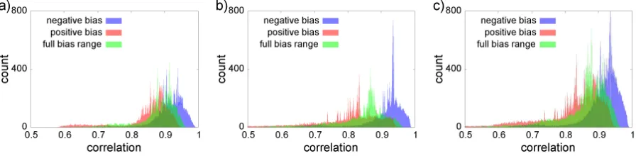
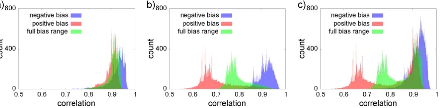
consid-FIG. 3: |V| ≤1 V relative brightness correlation histograms calculated by using 18144 tip orientations for: a) Wblunt tip, b) Wsharp tip. Part c) reports the sum of the histograms in

a) and b). The correlation histograms for the negative, positive and full bias ranges are

shown using Eq.(3) in the [0.5, 1] range with 0.001 resolution.

ered tungsten tip models in 18144 tip orientations and the sum of the two histograms in Fig. 3c). The maximal correlation between the experiment and simulations is found at

ap-proximately 0.97 in the negative and at approx. 0.95 in the positive bias range for both tips. However, we cannot conclude that the tip orientations belonging to the maximal correlation are the best since there is a large number of other orientations within a few percent from

the maximum correlation well above 0.9. Analyzing the correlation distribution, it is clearly seen that much more tip orientations provide better correlation values in the negative

com-pared to the positive bias range for both tip models. This effect is even more evident for the Wsharp tip, where the correlation distributions have two distinct peaks for the negative and

positive bias at around 0.93 and 0.66, respectively. The presented statistics for the relative

brightness correlation taking a large number of tip orientations confirm the significance of the findings of Ref. [11], where the simulated brightness profiles obtained at positive bias for the Wsharp tip model in high symmetry orientations resulted in much lower correlation

with the experiment than in the negative bias voltage range. No such large differences were found for the Wblunt tip at either bias polarities. This suggests that the Wblunt tip is more

likely to be present in a wide range of bias voltages in the experiment than the Wsharp tip.

The minimal correlation between the experimental and simulated brightness profiles is found at 0.55 for the Wsharp tip at positive bias voltages, whereas for the Wsharp tip at

negative bias voltages and for the Wblunt tip at all considered bias voltage ranges the minimal

correlation is above 0.7. Once more, this suggests a more likely Wblunt than Wsharp tip in

the experiment since various local rotations of the Wblunt tip do not give worse correlations

with the experiment than 0.7, whereas there are particular local rotations of the Wsharp tip

at positive bias voltages with much worse correlations.

The presented relative brightness correlation histograms provide information about the

distribution of the correlation values in terms of the number of simulated tip orientations within a particular correlation range with the experimental brightness data. This

presenta-tion of the correlapresenta-tion statistics, however, cannot tell which specific tip orientapresenta-tions give the best or worst correlations with the experiment. To assign the most or least likely orientations of the STM tip in the experiment for the given tip model, we need another representation

of the correlation data. Therefore, we complement our analysis by calculating correlation maps: r(Wblunt, θ0, φ0, ψ0) and r(Wsharp, θ0, φ0, ψ0).

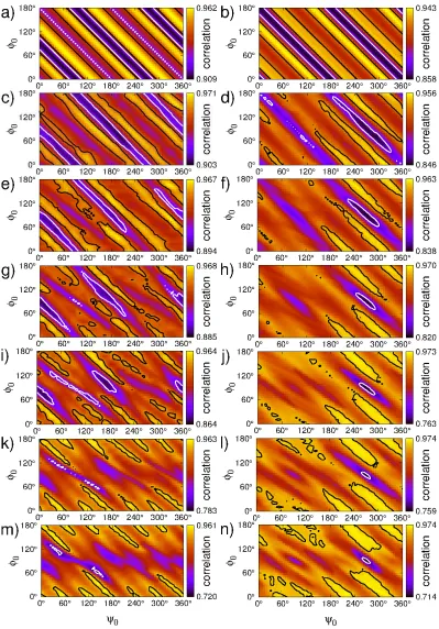
Figs. 4, 5 and 6 show the calculated relative brightness correlation maps for the two con-sidered tungsten tip models in the negative, positive and full bias voltage range, respectively.

r(φ0, ψ0) two-dimensional maps are shown as a function ofθ0. Note thatθ0 = 0◦ corresponds

to the same z-axis of the surface and the tip, and in this case φ0 and ψ0 denote the same

type of rotations around the common z-axis. As a result, we obtain striped r(φ0, ψ0)

corre-lation maps for θ0 = 0◦ [panels a) and b)]. For θ0 >0◦ these maps quickly change to show

more complicated correlation distributions [panels c)-n)]. Most importantly, Figs. 4, 5 and

6 show the most (least) likely tip orientations (θ0, φ0, ψ0) in the experiment in the given bias

interval corresponding to bright (dark) regions bounded by black (white) contours within 2% relative to the maximum (minimum) correlation value for each θ0 assuming the model

tip apex geometry. Overall, we find that the regions close to the maximal and minimal correlations can be differently affected by the bias range considered for the mapping for dif-ferent tip apex geometries. These results emphasize the importance of a large experimental

dataset for reliable application of the proposed procedure. Considering the favorable and unfavorable orientations for the given tip models, we find that the (φ0, ψ0) positions of the

indicated regions close to the maximum and minimum correlations in the r(φ0, ψ0) maps

are fairly stable with respect to the change of θ0. This means that the specific (φ0, ψ0)

Euler angles are representative for the likely (bright regions) and unlikely (dark regions) tip

orientations in the STM experiment, irrespective of θ0. Based on our results, we find that

the favored tip-sample relative orientations are far from being symmetric.

FIG. 4: -1 V ≤V <0 V negative bias range correlation analysis. Relative brightness correlation distributions r(θ0, φ0, ψ0) for Wblunt tip [first column: a), c), e), g), i), k), m)]

and Wsharp tip [second column: b), d), f), h), j), l), n)] for the following fixed θ0 angles:

a)-b) 0◦_{, c)-d) 5}◦_{, e)-f) 10}◦_{, g)-h) 15}◦_{, i)-j) 20}◦_{, k)-l) 25}◦_{, m)-n) 30}◦_{. Most (least) likely tip} orientations in the experiment in the given bias interval correspond to bright (dark)

regions bounded by black (white) contours within 2% relative to the maximum (minimum) correlation value in each subfigure assuming the model tip apex geometry.

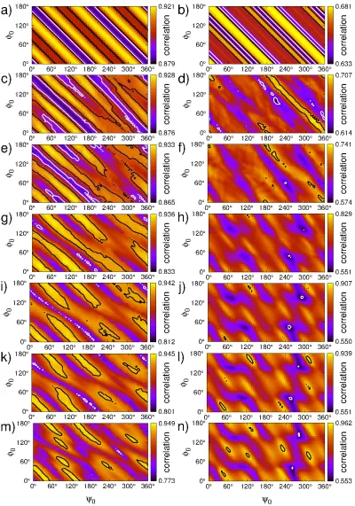
FIG. 5: 0 V < V ≤1 V positive bias range correlation analysis. Relative brightness correlation distributions r(θ0, φ0, ψ0) for Wblunt tip [first column: a), c), e), g), i), k), m)]

and Wsharp tip [second column: b), d), f), h), j), l), n)] for the following fixed θ0 angles:

a)-b) 0◦_{, c)-d) 5}◦_{, e)-f) 10}◦_{, g)-h) 15}◦_{, i)-j) 20}◦_{, k)-l) 25}◦_{, m)-n) 30}◦_{. Most (least) likely tip} orientations in the experiment in the given bias interval correspond to bright (dark)

FIG. 6: |V| ≤1 V full bias range correlation analysis. Relative brightness correlation distributions r(θ0, φ0, ψ0) for Wblunt tip [first column: a), c), e), g), i), k), m)] and Wsharp

tip [second column: b), d), f), h), j), l), n)] for the following fixed θ0 angles: a)-b) 0◦, c)-d)

5◦_{, e)-f) 10}◦_{, g)-h) 15}◦_{, i)-j) 20}◦_{, k)-l) 25}◦_{, m)-n) 30}◦_{. Most (least) likely tip orientations in} the experiment in the given bias interval correspond to bright (dark) regions bounded by

black (white) contours within 2% relative to the maximum (minimum) correlation value in each subfigure assuming the model tip apex geometry.

area ratios at fixed θ0 can be interpreted as the likelihood of favorable or unfavorable tip

orientations in the experiment assuming the considered tip geometry in the given bias range. The area ratios alone, however, are not sufficient to identify the most or least likely tip

orientations in the experiment since the maximum and minimum correlation values vary considerably depending on θ0.

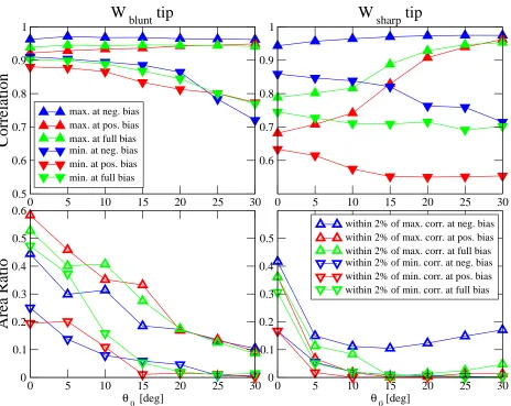
To further analyze the correlation maps in Figs. 4, 5 and 6, the evolutions of the maximum and minimum correlation values and the calculated area ratios with θ0 are reported in Fig.

7. This figure also allows comparison between the different bias voltage ranges and the

two considered tip models. We find that the maximum correlation is increasing and the minimum correlation is decreasing with increasingθ0 for all bias voltage ranges. This results

in a larger difference between the maximum and minimum correlations with increasing θ0.

It is interesting to note that the maximum correlation values are always larger than 0.9 for the Wblunt tip, whereas this is true only in the negative bias range for the Wsharp tip. In the

positive and full bias ranges the maximum correlation above 0.9 is achieved forθ0 ≥20◦, i.e.,

for a much smaller number of considered tip orientations. On the other hand, the minimum

correlation values are always smaller for the Wsharp compared to the Wblunt tip. These

findings clearly suggest that the Wblunt tip is more likely to be present in the experiment in

an enhanced bias voltage range than the Wsharp tip.

In Fig. 7, at negative bias voltages the two tips provide similar maximum correlation values as a function of θ0. In such case the area ratios can be used to decide which tip is

more likely in the experiment since the corresponding area ratios are proportional to the number of tip orientations within the maximum correlation, and such larger area ratios favor a given tip. We find that the area ratios are generally larger for the Wblunt compared to

the Wsharp tip. Area ratios close to the correlation maximum mean that more orientations

can provide better correlation values for the Wblunt than for the Wsharp tip. On the other

hand, area ratios close to the correlation minimum mean that more orientations provide correlations close to the minimum for the Wblunt compared to the Wsharp tip. This is,

however, not a problem in the present case since the minimum correlations are always larger

for the Wblunt compared to the Wsharp tip. Therefore, based on the number of favorable tip

orientations, we can also conclude that the blunt tungsten tip is indeed more likely in the experiment than the sharp tip in the |V| ≤1 V bias voltage range.

0 5 10 15 20 25 30 0.5 0.6 0.7 0.8 0.9 1

Correlation

max. at neg. bias max. at pos. bias max. at full bias min. at neg. bias min. at pos. bias min. at full bias

0 5 10 15 20 25 30 0.6

0.7 0.8 0.9 1

0 5 10 15 20 25 30

θ ₀ [deg] 0 0.1 0.2 0.3 0.4 0.5 0.6

Area Ratio

0 5 10 15 20 25 30

θ ₀ [deg] 0 0.1 0.2 0.3 0.4 0.5

within 2% of max. corr. at neg. bias within 2% of max. corr. at pos. bias within 2% of max. corr. at full bias within 2% of min. corr. at neg. bias within 2% of min. corr. at pos. bias within 2% of min. corr. at full bias

W

tip

W

tip

FIG. 7: Analysis of the correlation maps in Fig. 4 (at negative bias), Fig. 5 (at positive

bias) and Fig. 6 (at full bias) in the|V| ≤1 V bias range. Top row: The evolution of the maximum and minimum correlation value in ther(θ0, φ0, ψ0) maps with θ0. Bottom row:

The θ0-evolution of the area within 2% relative to the maximum and minimum correlation

values (respectively bounded by the black and white contours in Figs. 4, 5 and 6) in relation to the area of ther(φ0, ψ0) map (36×72). These area ratios at fixed θ0 can be

interpreted as the likelihood of favorable or unfavorable tip orientations in the experiment

assuming the considered tip geometry. Left and right parts respectively correspond to data obtained by Wblunt and Wsharp tip models.

with simulated brightness profiles obtained by taking the contributions of four extra next-neighbor atoms of the tip apex atom in the tunneling current calculations using the 3D-WKB

method. We find that the correlation maps are quantitatively very similar to those obtained by the one-apex tip for θ0 ≤ 20◦. For larger θ0-tilting the emergence of multiple tip apices

FIG. 8: |V| ≤0.3 V relative brightness correlation histograms calculated by using 18144 tip orientations for: a) Wblunt tip, b) Wsharp tip. Part c) reports the sum of the histograms

in a) and b). The correlation histograms for the negative, positive and full bias ranges are

shown using Eq.(3) in the [0.5, 1] range with 0.001 resolution.

distorts the simulated brightness profiles and consequently worsens the agreement with the experiment, manifesting as dramatically reduced correlation values (down to 0.35 atθ0 = 25◦

and 0.13 at θ0 = 30◦) for particular (φ0, ψ0) ranges. Based on this, we can conclude that

our findings are robust for θ0 ≤20◦, i.e. for a small tilting of the tip z-axis.

To investigate the effect of the bias voltage on the obtained results, we recalculated the

correlation statistics in the |V| ≤0.3 V bias voltage range that corresponds to the low bias regime used in typical STM imaging experiments of HOPG. This analysis used redefined negative (-0.3 V ≤V < 0 V, NV = 3), positive (0 V < V ≤ 0.3 V, NV = 3) and full (-0.3

V ≤ V ≤ 0.3 V, NV = 6) bias ranges. Fig. 8 shows the recalculated relative brightness

correlation histograms for the two considered tungsten tip models in 18144 tip orientations

and the sum of the two histograms in Fig. 8c). We find qualitatively similar results as in the |V| ≤1 V bias range reported in Fig. 3. The main differences in Fig. 8 in comparison to Fig. 3 are: i) there is a longer tail of the correlation distributions extending toward lower

values for both tips, resulting in much lower minimum correlations (e.g., 0.26 for the Wsharp

tip at positive bias voltages and 0.58 for the Wblunt tip at all bias ranges), ii) the maximum

correlations are increased to 0.99 at negative bias for both tips, iii) the difference between

the two distinct peaks of the correlation distributions for the negative and positive bias in case of the Wsharp tip is reduced, but still significant (above 0.1).

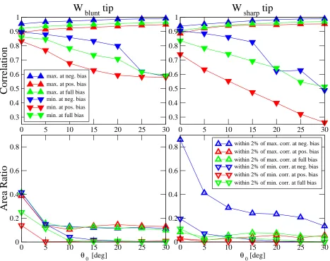
Fig. 9 shows the evolutions of the maximum and minimum correlation values and the

calculated area ratios withθ0obtained from ther(θ0, φ0, ψ0) correlation maps in the|V| ≤0.3

0 5 10 15 20 25 30 0.3 0.4 0.5 0.6 0.7 0.8 0.9 1

Correlation

max. at neg. bias max. at pos. bias max. at full bias min. at neg. bias min. at pos. bias min. at full bias

0 5 10 15 20 25 30 0.3 0.4 0.5 0.6 0.7 0.8 0.9 1

0 5 10 15 20 25 30

θ ₀ [deg] 0 0.2 0.4 0.6 0.8

Area Ratio

0 5 10 15 20 25 30

θ ₀ [deg] 0

0.2 0.4 0.6

0.8 within 2% of max. corr. at neg. bias

within 2% of max. corr. at pos. bias within 2% of max. corr. at full bias within 2% of min. corr. at neg. bias within 2% of min. corr. at pos. bias within 2% of min. corr. at full bias

W

tip

W

tip

FIG. 9: Extracted data from the correlation maps in the |V| ≤0.3 V bias voltage range. Top row: The evolution of the maximum and minimum correlation value in the

r(θ0, φ0, ψ0) maps with θ0. Bottom row: The θ0-evolution of the area ratio, for explanation

see the caption of Fig. 7. Left and right parts respectively correspond to data obtained by

Wblunt and Wsharp tip models.

in the low bias regime. However, the area ratios within 2% of the maximum correlation are systematically larger for the Wsharp than for the Wblunt tip in the negative bias range. Since

the maximum correlations are above 0.93 for for both type of tips in this bias interval, this suggests that more tip orientations of the Wsharp tip result in better agreement with the

experiment than of the Wblunt tip at low negative bias, -0.3 V ≤V < 0 V. The indications

of a favored Wblunt tip in the experiment are, however, not affected in the other considered

low bias regimes.

Although using larger bias ranges is better for the statistical analysis, the tip may become

unstable in the experiment at larger bias voltages, thus making the assignment of the tip

geometry and orientation more difficult. In general, we suggest that the primary decision for the quality of the STM tip in an experiment has to be based on the comparison between the

maximum and minimum relative brightness correlations between two (or more) tip models, and the secondary decisive factor should be the introduced area ratio measure that gives information on the number of likely or unlikely tip orientations.

IV. CONCLUSIONS

In scanning probe experiments the scanning tip is the source of one of the largest un-certainty as very little is known about its precise atomic structure and stability. Since the

atomic structure and electronic properties of the tip apex can strongly affect the contrast of STM images, it is very difficult to experimentally obtain predictive STM images in certain systems. To tackle this problem we proposed a statistical correlation analysis method to

ob-tain information on the local geometry and orientation of the tip used in STM experiments. We defined the relative brightness correlation of constant-current topographs between ex-perimental and simulated data, and analyzed it statistically for the HOPG(0001) surface in

combination with two tungsten tip geometries in 18144 orientations. The simulations were performed using the 3D-WKB electron tunneling theory based on first principles electronic

structure calculations. We find that a blunt tip model provides better correlation with the experiment for a wider range of tip orientations and bias voltages than a sharp tip model. A favored sharp tip is indicated at low negative bias only. From the correlation distribution

we proposed particular tip orientations that are most likely present in the STM experiment, and likely excluded other orientations. Importantly, we find that the favored relative

tip-sample orientations do not correspond to high symmetry setups that are routinely used in standard STM simulations. The demonstrated combination of large scale simulations with experiments is expected to open up the way for a more reliable interpretation of STM data in

ACKNOWLEDGMENTS

The authors thank E. Inami, J. Kanasaki, and K. Tanimura at Osaka University for

the experimental brightness data. Financial support of the Magyary Foundation, EEA and Norway Grants, the Hungarian Scientific Research Fund project OTKA PD83353, the Bolyai Research Grant of the Hungarian Academy of Sciences, and the New Sz´echenyi Plan

of Hungary (Project ID: T ´AMOP-4.2.2.B-10/1–2010-0009) is gratefully acknowledged. G. T. is supported by EPSRC-UK (EP/I004483/1). Usage of the computing facilities of the

Wigner Research Centre for Physics and the BME HPC Cluster is kindly acknowledged.

APPENDIX: 3D-WKB TUNNELING THEORY

M´andiet al. have developed an orbital-dependent electron tunneling model with arbitrary

tip orientations [10] for simulating scanning tunneling microscopy (STM) measurements within the three-dimensional (3D) Wentzel-Kramers-Brillouin (WKB) framework based on previous atom-superposition theories [13, 16, 17, 23–26]. Here, this method is briefly

de-scribed, which was used in the paper for the HOPG(0001) surface in combination with tungsten tips. The model assumes that electrons tunnel through a tip apex structure

con-sisting of a few atoms, and transitions between individual atoms of this tip apex structure and a suitable number of sample surface atoms, each described by the one-dimensional (1D) WKB approximation, are superimposed [13, 15]. Since the 3D geometry of the tunnel

junc-tion is considered, the method is a 3D-WKB atom-superposijunc-tion approach. The advantages, particularly computational efficiency, limitations, and the potential of the 3D-WKB method were discussed in Ref. [14].

The electronic structure of the surface and the tip is included in the model by taking the atom-projected electron density of states (PDOS) obtained by ab initioelectronic structure calculations [16]. The orbital-decomposition of the PDOS is necessary for the description

of the orbital-dependent electron tunneling [13]. The energy-dependent orbital-decomposed PDOS functions of theith sample surface atom with orbital symmetryσand thejth tip atom

with orbital symmetry τ are denoted by ni

Sσ(E) and n j

T τ(E), respectively. In the present

work σ ∈ {s, py, pz, px} atomic orbitals for the carbon atoms on the HOPG surface and

τ ∈ {s, py, pz, px, dxy, dyz, d3z2_−r2, d_xz, d_x2_−y2} orbitals for the apex atoms of blunt and sharp tungsten tips are considered. The total PDOS function is the sum of the orbital-decomposed contributions:

ni_S(E) =X

σ

ni_Sσ(E), (A4)

njT(E) =

X

τ

njT τ(E). (A5)

Note that a similar decomposition of the Green’s functions was reported within the linear

combination of atomic orbitals (LCAO) framework in Ref. [27].

Assuming elastic electron tunneling at temperature T = 0 K, the tunneling current at the tip apex position RT IP and bias voltage V is given by the superposition of atomic

orbital combinations between the sample and the tip (sum over σ and τ):

I(R_{T IP}, V) = X

i

X

j

X

σ,τ

I_στij (R_{T IP}, V). (A6)

One particular current contribution can be calculated as an integral in an energy window corresponding to the bias voltage V as

I_στij (RT IP, V) = ǫ2

e2

h

Z V 0 Tστ

E_FS +eU, V,dij

×ni_SσE_FS+eUnj_{T τ}E_FT +eU −eVdU. (A7) Here, e is the elementary charge, h is the Planck constant, and ES

F and EFT are the Fermi

energies of the sample surface and the tip, respectively. Theǫ2_e2_{/hfactor ensures the correct}

dimension of the electric current. The value of ǫ has to be determined by comparing the simulation results with experiments, or with calculations using standard methods, e.g., the

Bardeen approach [28]. In our simulations ǫ = 1 eV was chosen that gives comparable current values with those obtained by the Bardeen method [13] implemented in the BSKAN code [29, 30]. Note that the choice of ǫ has no qualitative influence on the reported results,

and a rigorous comparison between the 3D-WKB and Bardeen methods in relation to STM experiments performed on HOPG [12] was reported in Ref. [11].

In Eq.(A7), Tστ (E, V,dij) is the orbital-dependent tunneling transmission function, and

it gives the probability of the electron tunneling from theτ orbital of thejth tip atom to the

σ orbital of the ith surface atom, or vice versa, depending on the sign of the bias voltage.

The conventions of tip → sample tunneling at positive bias voltage (V >0) and sample →

tip tunneling at negative bias (V < 0) are used. The transmission probability depends on

the energy of the electron (E), the bias voltage (V), and the relative position of the jth tip atom and the ith sample surface atom (dij = RjT IP −Ri). Note that RT IP corresponds

to the position of the tip apex atom. The following form for the transmission function is

considered [10]:

Tστ

EFS +eU, V,dij

= exp{−2κ(U, V)|dij|}χ2σ(θij, φij)χ2τ(θij′ , φ′ij). (A8)

Here, the exponential factor corresponds to an orbital-independent transmission, where all

electron states are considered as exponentially decaying spherical states [23, 26, 31], and it depends on the distance between the jth tip atom and the ith surface atom, |dij|, and on

the vacuum decay,

κ(U, V) = 1 ¯

h

s

2m

ϕ

S+ϕT +eV

2 −eU

. (A9)

For using thisκan effective rectangular potential barrier in the vacuum between the sample

and the tip is assumed. ϕS and ϕT are the electron work functions of the sample surface

and the tip, respectively, m is the electron’s mass and ¯h the reduced Planck constant. The

remaining factors of Eq.(A8) are responsible for the orbital dependence of the transmission. They modify the exponentially decaying part according to the real-space shape of the elec-tron orbitals involved in the tunneling, i.e., the angular dependence of the elecelec-tron densities

of the atomic orbitals of the surface and the tip is taken into account as the square of the real spherical harmonics χσ(θij, φij) and χτ(θij′ , φ′ij), respectively. It is important to note that

the angles are given in the respective local coordinate system of the surface (without primes) and the tip (denoted by primes). This distinction of the local coordinate systems is crucial to describe arbitrary tip orientations that correspond to a rotation of the tip coordinate

system by the set of Euler angles (θ0, φ0, ψ0) with respect to the surface coordinate system

[10]. The transformation between a vector defined in the local coordinate system of the tip,

(x′_{, y}′_{, z}′_{), and a vector defined in the local coordinate system of the sample, (x, y, z), is} given by       x′ y′ z′      

=R(θ0, φ0, ψ0)       x y z       , (A10)

with the rotation matrix:

R(θ0, φ0, ψ0) = (A11)

      

cosφ0cosψ0−sinφ0sinψ0cosθ0 cosφ0sinψ0+ sinφ0cosψ0cosθ0 sinφ0sinθ0

−sinφ0cosψ0−cosφ0sinψ0cosθ0 −sinφ0sinψ0+ cosφ0cosψ0cosθ0 cosφ0sinθ0

sinψ0sinθ0 −cosψ0sinθ0 cosθ0

       .

The polar and azimuthal angles (θ(_ij′), φ(_ij′)) given in both real spherical harmonics in Eq.(A8) correspond to the tunneling direction, i.e., the line connecting the ith surface atom and the jth tip atom, as viewed from their local coordinate systems (denoted by no prime and

prime, respectively), and they have to be determined for each surface atom-tip atom (i−j) combination from the actual tip-sample geometry. A schematic view of an STM tip with rotated local coordinate system by the Euler angles (θ0, φ0, ψ0) above the HOPG(0001)

3D-WKB and Bardeen methods in relation to STM experiments performed on HOPG, see

Ref. [11].

REFERENCES

[1] M. Herz, F.J. Giessibl, J. Mannhart, Probing the shape of atoms in real space, Phys. Rev. B

68 (2003) 045301/1-7.

[2] A.N. Chaika, S.S. Nazin, V.N. Semenov, S.I. Bozhko, O. L¨ubben, S.A. Krasnikov, et al.

Selecting the tip electron orbital for scanning tunneling microscopy imaging with sub-angstrom

lateral resolution, EPL 92 (2010) 46003/p1-p6.

[3] A.N. Chaika, S.S. Nazin, V.N. Semenov, N.N. Orlova, S.I. Bozhko, O. L¨ubben, et al. High

resolution STM imaging with oriented single crystalline tips, Appl. Surf. Sci. 267 (2013)

219-223.

[4] G. Rodary, J.-C. Girard, L. Largeau, C. David, O. Mauguin, Z.-Z. Wang, Atomic structure

of tip apex for spin-polarized scanning tunneling microscopy, Appl. Phys. Lett. 98 (2011)

082505/1-3.

[5] L. Gross, N. Moll, F. Mohn, A. Curioni, G. Meyer, F. Hanke, et al. High-resolution molecular

orbital imaging using a p-wave STM tip, Phys. Rev. Lett. 107 (2011) 086101/1-4.

[6] C.J. Chen, Tunneling matrix elements in three-dimensional space: The derivative rule and

the sum rule, Phys. Rev. B 42 (1990) 8841-8857.

[7] B. Siegert, A. Donarini, M. Grifoni, The role of the tip symmetry on the STM topography of

π-conjugated molecules, Phys. Stat. Sol. B 250 (2013) 2444-2451.

[8] A.J. Lakin, C. Chiutu, A.M. Sweetman, P. Moriarty, J.L. Dunn, Recovering molecular

orien-tation from convoluted orbitals, Phys. Rev. B 88 (2013) 035447/1-8.

[9] J.H.A. Hagelaar, C.F.J. Flipse, J.I. Cerd´a, Modeling realistic tip structures: Scanning

tunnel-ing microscopy of NO adsorption on Rh(111), Phys. Rev. B 78 (2008) 161405/1-4.

[10] G. M´andi, N. Nagy, K. Palot´as, Arbitrary tip orientation in STM simulations: 3D WKB

theory and application to W(110), J. Phys. Condens. Matter 25 (2013) 445009/1-10.

[11] G. M´andi, G. Teobaldi, K. Palot´as, Contrast stability and ’stripe’ formation in scanning

tunneling microscopy imaging of highly oriented pyrolytic graphite: the role of STM-tip

ori-entations, J. Phys. Condens. Matter 26 (2014) 485007/1-11.

[12] G. Teobaldi, E. Inami, J. Kanasaki, K. Tanimura, A.L. Shluger, Role of applied bias and tip

electronic structure in the scanning tunneling microscopy imaging of highly oriented pyrolytic

graphite, Phys. Rev. B 85 (2012) 085433/1-15.

[13] K. Palot´as, G. M´andi, L. Szunyogh, Orbital-dependent electron tunneling within the atom

superposition approach: Theory and application to W(110), Phys. Rev. B 86 (2012)

235415/1-11.

[14] K. Palot´as, G. M´andi, W.A. Hofer, Three-dimensional Wentzel-Kramers-Brillouin approach

for the simulation of scanning tunneling microscopy and spectroscopy, Front. Phys. 9 (2014)

711-747.

[15] K. Palot´as, W.A. Hofer, L. Szunyogh, Theoretical study of the role of the tip in enhancing

the sensitivity of differential conductance tunneling spectroscopy on magnetic surfaces, Phys.

Rev. B 83 (2011) 214410/1-9.

[16] K. Palot´as, W.A. Hofer, L. Szunyogh, Simulation of spin-polarized scanning tunneling

mi-croscopy on complex magnetic surfaces: Case of a Cr monolayer on Ag(111), Phys. Rev. B 84

(2011) 174428/1-11.

[17] K. Palot´as, W.A. Hofer, L. Szunyogh, Simulation of spin-polarized scanning tunneling

spec-troscopy on complex magnetic surfaces: Case of a Cr monolayer on Ag(111), Phys. Rev. B 85

(2012) 205427/1-13.

[18] K. Palot´as, Prediction of the bias voltage dependent magnetic contrast in spin-polarized

scan-ning tunneling microscopy, Phys. Rev. B 87 (2013) 024417/1-11.

[19] G. M´andi, K. Palot´as, STM contrast inversion of the Fe(110) surface, Appl. Surf. Sci. 304

(2014) 65-72.

[20] P. Nita, K. Palot´as, M. Ja lochowski, M. Krawiec, Surface diffusion of Pb atoms on the

Si(553)-Au surface in narrow quasi-one-dimensional channels, Phys. Rev. B 89 (2014) 165426/1-6.

[21] M. Ondr´aˇcek, P. Pou, V. Rozs´ıval, C. Gonz´alez, P. Jel´ınek, R. P´erez, Forces and currents in

carbon nanostructures: Are we imaging atoms?, Phys. Rev. Lett. 106 (2011) 176101/1-4.

[22] J.M. Blanco, C. Gonz´alez, P. Jel´ınek, J. Ortega, F. Flores, R. P´erez, First-principles

sim-ulations of STM images: From tunneling to the contact regime, Phys. Rev. B 70 (2004)

[23] J. Tersoff, D.R. Hamann, Theory of the scanning tunneling microscope, Phys. Rev. B 31

(1985) 805-813.

[24] H. Yang, A.R. Smith, M. Prikhodko, W.R.L. Lambrecht, Atomic-scale spin-polarized scanning

tunneling microscopy applied to Mn3N2(010), Phys. Rev. Lett. 89 (2002) 226101/1-4.

[25] A.R. Smith, R. Yang, H. Yang, W.R.L. Lambrecht, A. Dick, J. Neugebauer, Aspects of

spin-polarized scanning tunneling microscopy at the atomic scale: experiment, theory, and

simu-lation, Surf. Sci. 561 (2004) 154-170.

[26] S. Heinze, Simulation of spin-polarized scanning tunneling microscopy images of nanoscale

non-collinear magnetic structures, Appl. Phys. A 85 (2006) 407-414.

[27] N. Mingo, L. Jurczyszyn, F.J. Garcia-Vidal, R. Saiz-Pardo, P.L. de Andres, F. Flores, et

al. Theory of the scanning tunneling microscope: Xe on Ni and Al, Phys. Rev. B 54 (1996)

2225-2235.

[28] J. Bardeen, Tunnelling from a many-particle point of view, Phys. Rev. Lett. 6 (1961) 57-59.

[29] W.A. Hofer, Challenges and errors: interpreting high resolution images in scanning tunneling

microscopy, Prog. Surf. Sci. 71 (2003) 147-183.

[30] K. Palot´as, W.A. Hofer, Multiple scattering in a vacuum barrier obtained from real-space

wavefunctions, J. Phys. Condens. Matter 17 (2005) 2705-2713.

[31] J. Tersoff, D.R. Hamann, Theory and application for the scanning tunneling microscope, Phys.

Rev. Lett. 50 (1983) 1998-2001.