The influence of fetch on the response of surface currents to wind studied by HF ocean surface radar

MALCOLML. HERON

Marine Geophysical Laboratory, James Cook University, and AIMS@JCU, Townsville, Queensland, Australia

(Manuscript received 4 October 2006, in final form 5 October 2007)

ABSTRACT

The momentum transfer from wind to sea generates surface currents through both the wind shear stress and the Stokes drift induced by waves. This paper addresses issues in the interpretation of HF radar measurements of surface currents and momentum transfer from air to sea. Surface current data over a 30-day period from HF ocean surface radar are used to study the response of surface currents to wind. Two periods of relatively constant wind are identified—one for the short-fetch condition and the other for the long-fetch condition. Results suggest that the ratio of surface current speed to wind speed is larger under the long-fetch condition, while the angle between the surface current vector and wind vector is larger under the short-fetch condition. Data analysis shows that the Stokes drift dominates the surface currents under the long-fetch condition when the sea state is more mature, while the Stokes drifts and Ekman-type currents play almost equally important roles in the total currents under the short-fetch condition. The ratios of Stokes drift to wind speed under these two fetch conditions are shown to agree well with results derived from the empirical wave growth function. These results suggest that fetch, and therefore sea state, signifi-cantly influences the total response of surface current to wind in both the magnitude and direction by variations in the significance of Stokes drift. Furthermore, this work provides observational evidence that surface currents measured by HF radar include Stokes drift. It demonstrates the potential of HF radar in addressing the issue of momentum transfer from air to sea under various environmental conditions.

1. Introduction

Ocean surface currents are dominant features that impact maritime industries as well as the monitoring of climate and weather. The surface currents are coupled to the atmosphere by wind stress and momentum trans-fer, and to the deep ocean by eddy viscosity and mo-mentum transfer. The main physical processes that de-termine the speed and direction of currents at and near the surface are Stokes drift, resulting from nonlineari-ties in the surface gravity waves, and Ekman dynamics, resulting from viscosity and Coriolis forces related to the rotation of the earth. In the numerical hydrody-namic modeling of ocean currents, the effect of Stokes drift is often not considered and the knowledge about wind stress is inadequate, both of which would cause

significant error in the results. Some work (Paduan and Shulman 2004) has been done to reduce numerical modeling error by using the HF radar data to improve the way wind forcing is introduced into the models. This has been achieved by assimilating the surface current data provided by HF radar into the modeling. HF radar is also used in the present study, but the emphasis in the present work is on investigating the relationship be-tween surface currents and the wind under different conditions to provide more insight into the physical processes involved, which will benefit surface current prediction and improve accuracy in numerical model-ing.

The response of surface currents to wind has two components: surface currents caused by momentum transfer through wind shear stress, and the Stokes mass transport. The former is explained by Ekman theory (Stewart 2005) and indicates a quadratic relation be-tween the surface wind drift currents and the wind; the latter is caused by the nonlinear character of waves

Corresponding author address: Yadan Mao, School of Engi-neering, James Cook University, Townsville 4811 QLD, Australia. E-mail: [email protected]

DOI: 10.1175/2007JPO3709.1

© 2008 American Meteorological Society

generated by wind (LeBlond and Mysak 1978) and in-dicates a linear relation between the Stokes drift and the wind. The momentum transfer from the wind into the ocean is through both wind shear stress and wave generation. Therefore, these two components are inde-pendent of each other, but work together to generate the current response. In different conditions, they play different roles.

As noted by Kirwan et al. (1979), resolving wind and wave drift components from each other and from a larger-scale main flow is a difficult experimental prob-lem. Most laboratory and field investigations have fo-cused on just one component.

Some exceptions include the analysis of Kirwan et al. (1979) and Wu (1983). The analysis of Kirwan et al. incorporated both of these two components. They found that linear theory was superior to the quadratic theory in explaining their data. However, because of some logistical compromises and uncertainty about the effect of wind drag on the exposed part of the buoy, they were unable to determine the role that Stokes drift played in the surface currents. In the study of Wu (1983), based on the wind-drag coefficient from labo-ratory experiments, and wave data compiled by Wiegel (1964), surface currents caused by wind stress and Stokes drift are calculated from empirical functions. However, both the wind and surface currents are treated as scalar and no angle relation was included in the analysis. In addition, the scarcity of the wave data used may have resulted in an inaccuracy of the wave parameters. The fetch-limited laboratory conditions in-hibit the contribution of Stokes drift to the total cur-rents.

Ekman’s theory predicts that the angle between the wind-driven surface current vector and the wind vector is 45°. This is derived under the assumption of a con-stant vertical eddy viscosity for steady wind-driven cur-rents in an infinitely homogenous ocean. This 45° angle relation is generally considered to be on the high side in field observations (Madsen 1977). The shortcomings of a constant vertical eddy viscosity have long been rec-ognized, and as a result the simple Ekman model has been extended to include variable eddy viscosity as well as boundary layers.

However, Stokes drift generated by waves also has an effect on the angle relation between the total surface drift currents and the wind. The study done by Lewis and Belcher (2003) demonstrates that the inclusion of the Stokes drift is the key to reconciling the discrepan-cies in the angular deflections of the steady-state cur-rents. Polton et al. (2005) also found that the surface current direction is affected by the presence of ocean waves. These studies are based on adding the influence

of Stokes drift into the Ekman model, and their ana-lytical solution agrees well with the current profiles from previously published observational data and agrees better than the standard Ekman model.

Stokes drift is different under different sea states and this is reflected in the total response of the surface cur-rent to wind. Using data from HF ocean surface radar, this study aims to focus on the influence of fetch on the surface current response to wind and ascertain the role that Stokes drift and wind stress play in generating sur-face currents under different fetch conditions. HF radar data have the advantage over drifter data in studying the response of surface current to wind because the error introduced by the wind acting directly on buoys is excluded.

There has been some controversy about the ability of HF surface radar to measure Stokes drift. Theoretical-ly, Creamer et al. (1989) described an approximation scheme that reproduces the effect of the lowest-order nonlinear behavior of surface waves, and captures im-portant features of short waves interacting with longer waves. Their results indicate that the surface currents measured by the HF radar should respond to Stokes drift from all waves with wavelengths longer than the Bragg waves. Many recent research projects were con-ducted with the assumption that Stokes drift is present in the HF radar surface current data (Graber and Haus 1997; Gremes-Cordero et al. 2003; Chapron et al. 2005; Ullman et al. 2006). Ullman et al. (2006) used two ranges of the Coastal Ocean Dynamics Applications Radar (CODAR) measurements with different effec-tive depths (⬃0.5 and⬃2.4 m), and compared the radar data with the drifters at a depth of 0.65 m. The com-parison suggests the existence of Stokes drift in the HF radar data and the importance of effective depth of radar measurements.

We approached the above issues by identifying two typical fetch conditions with approximately the same wind speed, and comparing the difference in current response under these two conditions. The differences in current response to wind under these two typical fetch conditions suggest that not only is Stokes drift present in the HF radar measurement, but also that fetch plays a significant role in the response of surface current to wind by varying the magnitude of Stokes drift under different sea states.

2. Experiment

a. Site

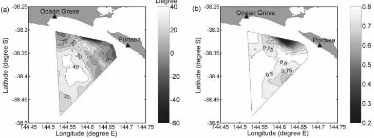
tool at James Cook University, and uses an eight-ele-ment antenna array for both transmit and receive modes. A pulse modulation is used and a transmit–re-ceive switch is used to change from a high-energy trans-mit pulse to a low-noise receiver after each transtrans-mit pulse. The radar stations were set up at Portsea (38°20⬘03.6⬙S, 144°42⬘16.9⬙E) and Ocean Grove (38°16⬘20.1⬙S, 144°31⬘01.4⬙E) in Bass Strait, near the entrance to Port Phillip Bay in Victoria, Australia. The area in which surface current maps are produced ranges from 38.3° to 38.5°S latitude, and from 144.5° to 144.7°E longitude, with the grid points shown as aster-isks in Fig. 1a. The radar data archive consists of surface current vectors every hour at each of the 269 grid points within this area for a 1-month period, from 27 June 2001 to 26 July 2001.

The bathymetry in the near-coastal zone is shown in Fig. 1a. Five weather stations are located along the coast around the study area—two on the right side, two on the left side, and one inside the bay. Comparison among the wind records suggests that wind is quite uni-form in the study area during the study period. Corre-lations of the wind data from each of these weather stations with the current data are all significant, with the highest correlation obtained from the weather sta-tion nearest to our study area, which is the one at the South Channel Island (marked as SCI in Fig. 1a). Therefore, wind data from an anemometer located 10 m above sea level on South Channel Island were used. Figure 1b shows the study area in a wider perspective and the two typical fetch conditions under which cur-rent response to wind will be compared.

b. Results

The experiment was carried out by recording hourly values of surface currents for 30 days and mapping sur-face current vectors at the 269 grid points. Over the 30-day duration, only one hourly dataset was lost, be-cause of environmental reasons.

The 10 grid points highlighted with circles at the south end of the mapped area had currents dominated by winds and all behaved in a similar way to wind changes. As will be mentioned later, these 10 grid points are selected for studying surface current re-sponse to wind under different fetch conditions. Figure 2 shows a typical time series of current at one of the grid points.

The high-frequency variation of the current is caused mainly by tides, while the low-frequency variation of the current is dominated by winds. Tidal analysis shows thatK1andM2are the dominant tidal components. By

filtering the surface current data with a 25-h boxcar filter, tide-generated currents are almost completely re-moved.

Hourly wind data were taken at South Channel Is-land for the 30-day period and the raw values are shown in Fig. 3.

3. Surface current response to wind

a. Overall response over the whole time series

Sea surface currents are generated by tides, winds, and other factors, such as geostrophic pressure gradi-ents and density gradigradi-ents. Currgradi-ents are also influenced by bottom friction, land boundaries, and water flowing FIG. 1. Map of the study area (a) land (shaded), data grid points (asterisks), and bathymetry contours (m); two

into and out of rivers or bays. To evaluate the signifi-cance of wind in generating surface currents in our study area, a correlation analysis was conducted be-tween the wind and filtered surface currents over the whole time series.

First both the wind data and the current data are filtered with 25-h boxcar low-pass filter. Let␪(t) be the angle between surface current vectorC(t) and the wind vectorW(t) at each time, and assume that the observed surface current is made up of a component CW(t) re-sponding to wind and a residualCR(t). If␾is the angle between vectorCW(t) and the wind vectorW(t), and␾ is assumed to be constant over the whole time series, then the component ofC(t) in the direction ofCW(t) at each time is |C(t)| cos[␪(t)⫺␾]. The assumption that␾ is constant over the entire duration allows ␾ to vary with locations (e.g., for different bathymetry), but does not allow ␾ to change with wind speed or direction. Later on, when analyzing the influence of fetch on the response of surface current to wind, this condition on␾ is relaxed.

The time series of |C(t)| cos(␪(t)⫺␾) is correlated with the time series of wind speed |W(t) | . By varying␾ from ⫺180° to 180°, the highest correlation between |C(t) | cos[␪(t)⫺␾] and |W(t)| is found, and the corre-sponding␾is assumed to be the overall direction rela-tion betweenCW(t) andW(t) over the whole time se-ries.

In performing the correlation analysis, a time shift was also considered. Figure 4 shows the correlation re-sults for 1 of the 10 selected grid points. The correlation coefficient is plotted as a contour with a varying angle

␾and time shifts.

Results show that the highest correlation coefficient for currents at this grid point and the wind is found at zero time shift and at an angle of ␾ ⫽20°. Figure 5a shows the correlation coefficient at zero time shift as angle␾varies, and Fig. 5b shows the correlation coef-ficient versus time shift when␾is 20°. Comparing the results of several points on the current maps, it is found that the highest correlation coefficient almost always occurs at about zero time shift, but at different values of angle␾. Therefore, we used zero time shift to find the value of␾at each grid point on the map. The values of

␾ and the corresponding maximum correlation coeffi-cient are shown in Figs. 6a,b, respectively.

FIG. 3. Wind data from an anemometer located on SCI,

refer-ence time is 1700 Australian eastern standard time (UTC⫹10) 27 Jun 2001: (top) east and (bottom) north component.

FIG. 4. Contours of correlation coefficient between |C(t) | cos(␪(t)⫺␾) and |W(t) | at one typical southern grid point vs␾ and time shift.

Figure 6a is the contour of ␾ values optimized for maximum correlation. The angle is defined in a way that positive values indicate that the current is on the left side of the wind. Figure 6a suggests that for most areas,␾[i.e., the angle between current responseCW(t) and the windW] is within the range of 10°–45°, which is in agreement with other observational results (Huang 1979). The angle appears to decrease for grid points near to the coast, which can be explained by the larger effect of bottom friction there. For areas near the en-trance of Port Phillip Bay, the value of␾varies widely and is often outside this range. Here, the surface cur-rents appear to respond to flow into and out of the bay on the surface current map.

Figure 6b shows the contour of correlation coeffi-cient corresponding to the optimized␾values shown in Fig. 6a. It is shown that, except for areas near the en-trance of Port Phillip Bay, the filtered current is highly correlated with wind for most of the study area, with a

correlation coefficient around 0.8. For the selected 10 grid points, after removing the effect of tide and wind, the residual current is found to be very small and be-haves like noise (Mao et al. 2007). Therefore, it is con-sidered that wind-generated currents dominate over other factors, such as geostrophic large-scale currents, for this part of the study area during this period of time. Figures 6a,b reveal the overall response of surface current to wind considering the whole time series; the linear correlation conducted over the whole time series is mainly aimed at finding the significance of wind in generating surface currents. The high correlation sug-gests that the wind is the dominant force in generating the filtered surface current for the grid points at the southern end of the current map.

Therefore, when we later investigate the influence of fetch on the response of surface current to wind in the southern end of the current map, the filtered surface current is considered to be generated by wind only. We

FIG. 6. Contours related to the response of surface current to wind over the whole time series; (a) the ␾value is optimized for maximum correlation. Positive angle indicates that the responding current is on the left of the wind. (b) The correlation coefficient between the surface current and wind corresponding to the optimized direction relation in (a) is given.

FIG. 5. Profile of the correlation coefficient corresponding to Fig. 4: (a) correlation coefficient at zero

are interested in how fetch influences the response of surface current to wind. To this end, we need to identify periods that represent a variety of fetch conditions with reasonably stable wind.

b. Response under long- and short-fetch periods

After being filtered with a 25-h boxcar low-pass fil-ter, the wind time series is shown in Figs. 7a,b in terms of speed and direction, respectively. The angle is de-fined trigonometrically, anticlockwise from east, and it shows the vector wind direction.

Given Figs. 7a,b and the geography map of Fig. 1b, we identified the period (230–320 h) when the wind was relatively constant in speed and direction over a long fetch, in addition to another period (420–500 h) over a short fetch. As will be mentioned later, the wave growth during the first 36 h of the long-fetch period is duration limited. Because we are mainly concerned about the influence of fetch, the interval of 270–320 h in the time series is chosen to represent the long-fetch periods. The short- and long-fetch periods are marked with dashed lines in Fig. 7. For the long-fetch section, the fetch is around 380 km; the mean speed of wind is 8.4 m s⫺1, with a standard deviation of 0.8 m s⫺1; and the mean direction of the wind vector is 149.9°, anti-clockwise from the east, with a standard deviation of 6.3°. For the short-fetch section, the fetch is around 30 km; the mean wind speed is 9.8 m s⫺1_{, with a standard}

deviation of 0.7 m s⫺1_{; and the mean direction of the}

wind is⫺15.8°, anticlockwise from the east, with a stan-dard deviation of 12.4°.

The average ratio of surface current speed AC to

wind speed U10 measured at 10 m above sea level is

shown in Fig. 7c with error bars marked as dotted lines. The errors of the current speed are calculated by the standard deviation over the 10 grid points divided by the square root of the number of grid points; the errors of the wind speed are calculated by the standard devia-tion over the adjacent 10-h period divided by the square root of the number of hours. Comparing Fig. 7a with Fig. 7c, it can be seen that large error bars generally correspond to low wind speeds. Ratio values that are unreasonably large also have large error bars and there-fore can be ignored. For the selected long- and short-fetch periods, the error bar is small, and hence the ratio values are significant. The average ratioAC/U10is 0.021

for the long-fetch period and 0.015 for the short-fetch period.

Typical maps of surface currents under the long- and short-fetch conditions are shown in Figs. 8a,b, respec-tively. The currents at the southern end of the mapped area behave uniformly and appear to respond mainly to the wind. At the northern end of the map, the currents are complex and appear to respond to the flow into and out of Port Phillip Bay. For the middle area, the cur-rents follow the bathymetry lines. This is reasonable, because the bathymetry gradients around the 60-m bathymetry line are large and variable; areas with bot-toms shallower than 60 m have larger bathymetry gra-dients. As depth increases, the gradients become smaller. Therefore, for areas near the coast with bathymetry shallower than 60 m, the currents are steered along the bathymetry contours.

The criteria we adopt here in choosing the grid points to study the influence of fetch on surface currents are as follows: 1) a high correlation with the wind (with cor-relation coefficient⬎0.8), 2) reasonably deep water and distant from the coast, and 3) far from the area with large bathymetry gradients. Therefore, only 10 points, as highlighted in Fig. 1, are chosen to study current response to wind under the short- and the long-fetch conditions. As shown in Fig. 6b, for these 10 grid points, the surface current is highly correlated with the wind, with the correlation coefficient higher than 0.8.

Comparing Figs. 8a,b for the selected 10 grid points, it is noticeable that the angle between the surface cur-rent and the wind is smaller in the long- than in the short-fetch condition. Because the current map shows the current only at a particular time, the difference in direction relation might not be representative of other times. Therefore, the direction relation averaged over the 10 selected grid points is shown in Fig. 9 as time series over the long- and the short-fetch periods. The errors of current direction and wind direction are cal-culated in the same way as for current speed and wind FIG. 7. The selected long- and short-fetch periods from (a) time

speed in Fig. 7. The condition on␾is now relaxed;␾is the angle between surface currents and wind averaged over the 10 selected grid points and is assumed to vary with fetch conditions: it is not constant as before over the entire 30-day duration.

As shown in Fig. 9, for the long-fetch period, the angle␾between surface currents and wind ranges from

6.8° to 19.9°, with an average of 14.4° and standard deviation of 3.8°. For the short-fetch period, the angle ranges from 17.8° to 36.2°, with an average of 24.4° and standard deviation of 4.9°. On average, the angle ␾ between surface currents and wind is 10° larger in the short- than in the long-fetch conditions.

Because the grid points remain the same under the

FIG. 9. (left) Direction of the wind vector and surface current vector over the (top) long- and (bottom) short-fetch periods; the angle is measured anticlockwise from the east. (right) Direction difference of surface current and wind over the long- and short-fetch periods; positive angle means the current vector is on the left side of the wind vector.

long- and the short-fetch conditions, factors such as ge-ography, bottom friction, and vertical eddy viscosity that may influence the value of ␾ are assumed to re-main the same in the long- and short-fetch conditions. Therefore, the difference in the value of␾under these two conditions can be attributed to the difference in wind fetch conditions.

In summary, the above results suggest that the ratio of the surface current speed to wind speed AC/U10 is

larger under long- than short-fetch conditions. Also, the angle ␾ between the surface current and the wind is smaller under long- than short-fetch conditions.

To explain these differences, we need to understand that wind generates surface currents as a result of mo-mentum transfer through both wind stress acting di-rectly on the ocean surface and Stokes drift induced by the nonlinearity of waves. As the wave spectrum devel-ops with fetch, the magnitude of Stokes drift also varies with fetch.

4. Surface current components

The response of surface current to wind is composed of both Ekman-type currents generated by wind stress and the Stokes drift. The former is governed by Ekman theory and the latter is governed by Stokes mass trans-port theory.

a. Ekman-type currents

Assuming a steady, homogeneous, horizontal flow with friction on a rotating earth and constant vertical eddy viscosity, the speed of surface current is derived from the momentum equation as (Stewart 2005)

VE⫽

T

公

2

fAz

, 共1兲

whereTis the wind stress,␳wis the water density,f⫽

2␻sin␸is the Coriolis parameter,␻is the rotation rate of the earth,␻ ⫽7.292⫻10⫺5_{(rad s}⫺1_{), andA}

zis the

eddy viscosity. A value forAzcannot be obtained from

theory. Instead, it must be calculated from data col-lected in wind tunnels or measured in the surface boundary layer at sea.

According to Ekman theory, surface wind drift cur-rents are 45° to the left of the wind in the Southern Hemisphere.

Wind stressTcan be calculated from

T⫽␳aCDU10

2 _{, 共2兲}

whereCDis the drag coefficient,␳a is the air density.

Substituting (2) into (1), we obtain

VE⫽

␳aCDU10 2

公

2

fAz

. 共3兲

Many studies have been done to obtain the drag coef-ficientCD. A form given by Wu (1980) is

CD⫽共0.8⫹0.065U10兲⫻10⫺ 3_U

10⬎1 m s⫺ 1_.

共4兲 Garratt (1992) gives

CD⫽共0.75⫹0.067U10兲⫻10⫺ 3

. 共5兲

More recently, Yelland and Taylor (1996) give

CD⫽

冉

3.1

U10 ⫹ 7.7

U10 2

冊

⫺3

3ⱕU10ⱕ6 m s⫺ 1

CD⫽共0.60⫹0.07⫻U10兲⫻10⫺ 3

6ⱕU10ⱕ26 m s⫺ 1

.

共6兲 These findings suggest that at relatively high wind speed, the drag coefficient increases with the wind speed. Using (5), we calculate the ratio of standard de-viation ofCDversus the mean ofCDfor the long- and

short-fetch periods. The ratio is 4.1% for the long-fetch period and 3.6% for the short-fetch period. Therefore,

CDis regarded as relatively constant over the selected

fetch periods, and thus (3) suggests that a quadratic relation between VEandU10is a good approximation

for the relation between the wind-generated current speed and the wind speed.

b. Stokes drift

1) EXPRESSION OFSTOKES DRIFT

The Stokes drift can be expressed as (Bye 1967)

VS⫽␻a

2

the Stokes drift.

If m0 is the variance or total energy of the wave

record,␻pis the peak frequency of the spectrum, andX

is the fetch for the wave field, the corresponding non-dimensional termsm⬘0,␻⬘p, andX⬘can be expressed as

m⬘0⫽

g2_m 0

U10

4 , ␻⬘p⫽

U10␻p

g , X⬘⫽ gX

U10

2 , 共9兲

where g is gravity acceleration. Thus, the nondimen-sional fetch for our long-fetch period is about 54 000, and for the short-fetch period is about 3100.

The significant wave heightHsis defined as (Janssen

2004)

Hs⫽4

公

Hence, for significant wave amplitudea, we have

a⫽1

2Hs⫽2

公

and, from wave dispersion theory, we have

k⫽␻

2

g . 共12兲

Substituting (9), (11), (12) into (8) yields the magnitude of Stokes drift with respect to the nondimensional wave parameters

VS⫽4␻⬘p

3

m⬘0U10. 共13兲

Equation (13) suggests that at a certain wave develop-ment state, there is a linear relation between the surface Stokes drift and the wind speed.

2) INFLUENCE OF FETCH ON WAVE PARAMETERS To calculate Stokes drift, wave parameters need to be known. Much work has been done to establish the empirical functions of wave parameters versus nondi-mensional fetch (Dobson et al. 1989; Donelan et al. 1985; Hasselmann et al. 1973; Kahma 1981; Kahma and Calkoen 1992). All of these expressions are obtained under different circumstances: some are obtained from

Lake Ontario (Donelan et al. 1985),

m⬘0⫽8.415⫻10⫺ 7

X⬘0.76, ␻⬘p⫽11.6X⬘⫺

0.23

; 共15兲

North Atlantic open ocean (Dobson et al. 1989),

m⬘0⫽1.27⫻10⫺ 6

X⬘0.75, ␻⬘p⫽10.68X⬘⫺

0.24_{; 共16兲}

an average expression with error bars (Young 1999),1

m⬘0⫽min

再

共7.5⫾2.0兲⫻10⫺7X⬘0.8

共3.6⫾0.9兲⫻10⫺3

␻⬘p⫽max

再

共12.56⫾1.88兲X⬘⫺0.25

0.82⫾0.13

. 共17兲

The above fetch-limited Eqs. (14)–(16) apply only to short-fetch condition when the wave is in fast growth. Despite their differences, there is a common form that nondimensional wave energy and frequency are power functions of nondimensional fetch; it is only the coeffi-cient and the exponent that vary between the different models. All of the above expressions of wave param-eters are in agreement, with the expectation that as nondimensional fetch increases, wave energy increases and the peak frequency decreases.

Once the fetch and duration are long enough that the sea reaches a fully developed state for a given constant wind speed, waves will not continue to grow even when either the fetch or duration increase further. The non-dimensional parameters of this constant state are given as (Pierson and Moskowitz 1964)

m⬘0⫽3.64⫻10⫺ 3

, ␻⬘p⫽0.82. 共18兲

Between the short fetch with a stable wave growth rate and the long fetch, where waves cease to grow, there is a transition region where the growth rate gradually slows down. For this transition region, the above-mentioned fetch-limited wave growth formulas

do not apply, because these empirical formulas are de-rived from fitting to the data only in the short-fetch region.

Therefore, for the transition regime, we look for em-pirical functions that are derived by fitting to data for both short and long fetches. During World War II, Sverdrup and Munk (1944, 1946) compiled existing data from a number of sources, including the field and laboratory. Bretschneider (1952a,b) later augmented and refined the results. The results have been summa-rized in CERC (1973), and the growth curve became know as the Sverdrup–Munk–Bretschneider (SMB) curve:

m⬘0⫽5.0⫻10⫺

3_tanh2_{共0.0125X⬘}0.42_兲

␻⬘p⫽

0.833

tanh共0.077X⬘0.25_兲. 共19兲

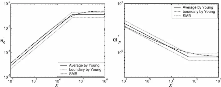
Nondimensional variance of wave energy and nondi-mensional peak frequency in (17) and (19) are plotted in Fig. 10. It can be seen that the transition region is from about 104_{to about 10}5_{in nondimensional fetch.}

Hence, the long-fetch condition in our study with a nondimensional fetch of 54 000 belongs to the transi-tion region in the fetch-limited wave growth regime. Therefore, for calculating the wave parameter in this region, it is better to use (19), which includes the tran-sition region, because it is derived from fitting to both long and short nondimensional fetches. The short-fetch condition with a nondimensional fetch of 3100 belongs to the short-fetch regime where the wave spectrum is in fast development. Wave parameters in this regime can be calculated using (14)–(17).

Because wave development is limited both by fetch and duration, the duration for wave development also needs to be considered. Because we are mainly con-cerned about the influence of fetch on the response of the surface current to wind, we need to know when the

wave is not duration limited. An empirical function was derived by CERC (1973) to calculate the duration for wave development,

␵⫽Kexp兵关A共lnX⬘兲2_{⫺BlnX⬘⫹C兴}1Ⲑ2_⫹DlnX⬘

其,

共20兲

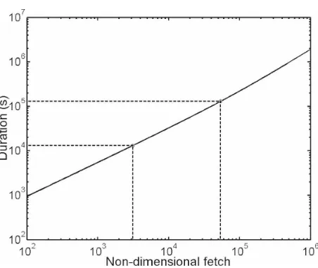
whereK⫽6.5882,A⫽0.0161,B⫽0.3692,C⫽2.2024, andD⫽0.8798. Here,␵is the nondimensional duration needed for wave development as a function of nondi-mensional fetchX⬘. As shown in Fig. 11, the duration required for wave development increases with increas-ing nondimensional fetch. The duration needed for wave development for the long- and short-fetch periods is marked in Fig. 11 as dashed lines.

For the short-fetch section, the wave growth will be duration limited for the first 3.6 h; for the long-fetch section, the wave growth will be duration limited for the first 36.1 h. Hence, for long fetches, the influence of duration on wave growth cannot be ignored. Because the long-fetch wind starts around 230 h in the time series, we choose 270–320 h to be the section for our long-fetch case, in order to exclude the effect of dura-tion on wave development.

5. Current data analysis

a. Determination of coefficients for Ekman-type surface currents and Stokes drift

As discussed above, the filtered surface current is mainly driven by the local wind, and the surface current is predominantly a combination of wind stress induced current vector VEand Stokes drift vectorVS. We ex-press the surface current in the following way:

V⫽VE⫹VS. 共21兲

FIG. 10. (left) Nondimensional total energym⬘0of wave record and (right) nondimensional frequency

With the quadratic and linear theories and the angle relations between the surface current and the wind ex-plained above, we have

VE⫽c1U10 2

冋

cos

冉

4

冊

冉

冊册

VS⫽c2U10共cos␣⫹isin␣兲, 共22兲

where U10 is the wind speed, ␣ is the angle of wind

anticlockwise to the east, andc1andc2are related with

drag coefficient and wave parameters, respectively. The real and imaginary parts represent components in the east and north directions, respectively. Substituting (22) into (21) yields the surface current equation,

u⫽a1U10

2_{共cos␣⫺sin␣兲⫹a}

2U10cos␣

␷⫽a1U10 2

共cos␣⫹sin␣兲⫹a2U10sin␣, 共23兲

whereuand␷are the observed east and north compo-nents of surface current, respectively. Here,a1anda2

are the two coefficients corresponding toc1and c2 in

(22);a1⫽

公

right side of (23) represents the component of the wind stress–generated surface current, including the qua-dratic relation and the 45° angle relation. The last term of (23) signifies the component of Stokes mass trans-port that is in the same direction as the wind, including the linear relation. Because the Stokes drift is in the wave direction, our assumption that the Stokes drift is in the wind direction implies that the wave is in the same direction as the wind. It is common practice to assume that the wave propagation direction agrees with the wind direction. Donelan et al. (1985) pointed out

that when the wind is not perpendicular to the land boundary, the gradient in the fetch about the wind di-rection is large and the wave didi-rection will not agree with the wind and will be biased toward the longer fetch. In our dataset, no wave information is available; otherwise, the dominant wave direction would be de-rived from the wave data. However, the shape of Lake Ontario, where Donelan et al. (1985) made their obser-vations, is quite elongated and enclosed. For our study area, the water body is within a fairly open geometry, and in the short-fetch duration the wind direction is rather perpendicular to the shoreline in the early half of the duration and is favorable for obtaining long fetch; hence, the effect of the water body geometry on the wave direction is expected to be small. Therefore, in applying Eq. (23), the problem is simplified by assum-ing that the direction of dominant wave agrees with the wind direction.

To ascertain the role VE and VS each play under different conditions, the least squares fitting process is applied to (23) to minimize the mean square speed re-sidual. The least squares fitting process was conducted on each of the 10 chosen points separately, with a set of

a1anda2values obtained for each grid point (Table 1).

The result of the fitting for 1 of the 10 grid points is shown in Fig. 12. The real current data and the model result derived from the value ofa1anda2at that point

are shown for the short- and long-fetch periods. Figure 12 also shows the current produced separately by wind stress and Stokes mass transport. It can be clearly seen that under the long-fetch condition, Stokes drift is dom-inant in generating the surface current, while under the short-fetch condition, Stokes drift is equally important as wind stress in generating the surface current. FIG. 11. Duration required for the full wave development vs

nondimensional fetch (CERC 1973); the dashed lines show the two durations for the long- and short-fetch conditions studied.

239 0.0006 0.0152 0.0231 0.0006 0.0082 0.0175 219 0.0007 0.0132 0.0294 0.0006 0.0089 0.0221 Average 0.0006 25 0.0150 0.0218 0.0006 0.0080 0.0205

Table 1 shows the least squares fitting results of co-efficients a1 and a2 for the 10 grid points during the

long- and short-fetch periods, as well as the average fitting error dc between the observed current and the model results. The modeling process here is done for each grid point in order to evaluate the generality of the value of coefficienta1anda2 so as to verify the

influ-ence of fetch on the values. The average coefficient value of these different points can be used for current prediction under the corresponding environmental con-dition.

Results show that the value of the coefficienta2for

Stokes drift is much smaller under the short- than long-fetch conditions. This suggests that under long-long-fetch conditions, resulting from more mature wave develop-ment, the influence of Stokes drift is much stronger than under short-fetch conditions. In contrast, the simi-larity of the value of the coefficienta1under these two

fetch conditions suggests that fetch condition does not have much influence on the wind stress–generated sur-face currentVE. As indicated by Eq. (3), the value of

公

2

wfAz)⫺

1/2

; therefore, the similarity ofa1under the two fetch

con-ditions suggests that the value of CDA⫺

1/2

z was not

af-fected much by the sea state because other parameters, such as water density ␳w, air density ␳a, and Coriolis

parameterf, were independent of fetch and assumed to be the same under different fetch conditions. The de-pendence of drag coefficientCDon sea state has been a

contentious issue; recently, some studies show that there is lack of evidence of this dependence (Janssen 1997; Yelland et al. 1998). In our study, a conclusion on whether the drag coefficientCDdepends on sea state

might be too early without further information of the variation of eddy viscosityAzwith fetch. However,

re-sults suggest that wind stress–generated surface current

does not have much dependence on the fetch condition, and as a result of wave development with fetch, Stokes drift increases with fetch, contributing to a larger ratio of total current speed to wind speedAC/U10.

b. Comparison with results derived from empirical wave growth functions

Finally, we are going to compare the values of the Stokes drift coefficientsa2derived from our data

analy-sis with those calculated from previously mentioned empirical equations. For short nondimensional fetches (⬍104_{), which apply to our short-fetch condition, (14)–}

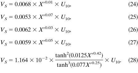
(17) and (19) can be used to calculate the wave param-eters. Substituting them into (13), the following equa-tions expressing Stokes drift as function of nondimen-sional fetchX⬘and wind speedU10are obtained:

VS⫽0.0068⫻X⬘

0.01_⫻U

10, 共24兲

VS⫽0.0053⫻X⬘

0.07_⫻U

10, 共25兲

VS⫽0.0062⫻X⬘

0.03

⫻U10, 共26兲

VS⫽0.0059⫻X⬘

0.05_⫻

U10, 共27兲

VS⫽1.164⫻10⫺

2_⫻tanh

2_{共0.0125X⬘}0.42_兲

tanh3共0.077X⬘0.25兲 ⫻U10. 共28兲

For the transition zone (which applies to the long-fetch condition), only (19) applies for the wave param-eters, thus Stokes drift can be calculated from (28). Figure 13 shows the ratioVS/U10derived from

empiri-cal Eqs. (24)–(28), and the values derived from our data analysis (coefficient a2 in Table 1) for different fetch

conditions.

It is shown that for the short-fetch condition, the values of VS/U10 derived from our data analysis are

FIG. 12. Model results at grid point 255 for (a) long- and (b) short-fetch periods; the total surface current speed

V(dashed), the observed surface current speedAC(solid), speed of the Ekman-type currentVE(dash dotted), and

within the range of values from empirical Eqs. (24)– (27), with an average of 0.8%; and for the transition region, the data are scattered around the value from (28) with an average of 1.5%. Therefore, the result of our analysis for surface currents induced by Stokes drift is in agreement with that calculated from the empirical wave growth functions.

The above results suggest that, because of wave de-velopment, Stokes drift is more significant in generat-ing surface currents under the long-fetch condition (transition region) than under the short-fetch condi-tion, resulting in smaller ␾ values and larger AC/U10

values for the long-fetch condition.

In addition, the curve from (28) in Fig. 13 suggests that after the transition region, as nondimensional fetch continues to increase, the ratioVS/U10decreases and is

about 1.22% when the wave is fully developed. Data representing large nondimensional fetch conditions are needed to verify this trend.

6. Conclusions

The theoretical approach by Creamer et al. (1989) indicates that the Stokes drift component measured by HF radar should be derived from all waves in the spec-trum that have wavelengths longer than that for the Bragg waves. The results of this paper indicate that the response of the ocean surface current to wind is a result of momentum transfer by both the wind stress and the Stokes mass transport. A quadratic law governs the

shows that, for most of the study area, wind dominates over other factors in generating surface currents (with correlation coefficient higher than 0.8). Current maps show that currents tend to follow the bathymetry con-tours in areas of high-bathymetry gradients. Ten grid points at the southern end where the filtered surface current is highly correlated with the filtered wind were chosen for the fetch analysis.

Two durations in the time series of wind represent the short- and long-fetch conditions. Wind data for these two durations are reasonably constant and strong. The ratio of surface current speed to wind speedAC/

U10 is higher under the long-fetch condition (average

value of 2.1%) than under the short-fetch condition (average value of 1.5%). In addition, the angle␾ be-tween the surface current and the wind is smaller under the long-fetch condition (average value of 14.4°) than under the short-fetch condition (average value of 24.4°).

Analysis of the data suggests that under the long-fetch condition, Stokes drift dominates the surface cur-rent, while under the short-fetch condition, wind stress and Stokes drift are almost equally important in gen-erating surface current. The ratios of Stokes drift to wind speedVS/U10obtained from data analysis

(coeffi-cienta2) are shown to agree well with the results

cal-culated from empirical wave growth functions. The long-fetch condition belongs to the transition region in the wave growth regime, while the short-fetch condi-tion belongs to the region with a high wave growth rate. Results show that the value ofVS/U10 is around 1.5%

under the long-fetch condition and 0.8% under the short-fetch condition. The larger value ofVS/U10under

the long- than the short-fetch condition accounts for the largerAC/U10 and the smaller␾ observed. In

con-trast, analysis results for the ratioVE/U

2

10, that is,

公

are similar in the short- and long-fetch conditions, sug-gesting that sea state does not affect the wind stress– generated current in a significant manner.

In the open sea, the wind fetch is often long, which is favorable for wave development. Hence, the Stokes drift is expected to dominate the surface drift in the FIG. 13. The value ofVS/U10from empirical functions and from

our data; values from (24)–(27) are shown as combined solid and dashed lines (dashed lines represent regions where these equa-tions do not apply). For the transition zone, the CERC (1973) line [Eq. (28)] is shown (solid). The asterisks (long fetch) and triangles (short fetch) represent the value from our data analysis (a2 in

open ocean. This explains why in the open sea, the linear relation between the surface current and the wind dominates over the quadratic relation, as found by Kirwan et al. (1979), and the angle between the current and wind is always smaller than the 45° that Ekman predicted (Madsen 1977). However, for areas under short fetch in the wave growth regime, the quadratic law for Ekman-type currents and the linear law for Stokes drift are about equally important in generating surface currents. These results imply that in the surface current prediction and 3D numerical modeling, varying the relation between current response and the wind according to different fetch condition will improve the outcomes.

This is an early result from 1 month of data in which only two periods satisfied the condition of constant wind direction at reasonably high, constant wind speed. Comprehensive data of surface currents and wind rep-resenting various nondimensional fetch conditions are needed to study in detail the variation of␾(the angle between the responding surface current and the wind) andAC/U10(the ratio of surface current speed to wind

speed) with fetch. It is also worth noting that no wave information was available in our study; otherwise, Stokes drift would have been derived independently from measured wave data. In the future, a more com-plete quantitative assessment of these ideas using mea-sured wave directional spectra should be carried out. This work provides some insight into the physics of the momentum transfer from air to sea and shows that HF radar measurements of surface currents include the ef-fect of Stokes drift. It demonstrates the value of HF ocean surface radar technology for carrying out surface current studies.

Acknowledgments.This work was supported by Aus-tralian Research Council SPIRT Grant C00002491. This work was carried out while Y. M. was a recipient of a Ph.D scholarship jointly sponsored by China Schol-arship Council and James Cook University. The wind data were provided by the Australian Bureau of Me-teorology. We wish to thank the Editor Dr. J. A. Smith for drawing our attention to Creamer et al. (1989). Valuable comments from the anonymous reviewers are also acknowledged.

REFERENCES

Bretschneider, C. L., 1952a: Revised wave forecasting relation-ships. Proc. Second Conf. on Coastal Engineering,ASCE, Council on Wave Research.

——, 1952b: The generation and decay of wind waves in deep water.Trans. Amer. Geophys. Union,33,381–389.

Bye, J. A. T., 1967: The wave drift current.J. Mar. Res.,25,95– 102.

CERC, 1973: Shore protection manual. U.S. Army Coastal Engi-neering Research Centre, Vol. 1, 35, 46.

Chapron, B., F. Collard, and F. Ardhuin, 2005: Direct measure-ments of ocean surface velocity from space: Interpretation and validation. J. Geophys. Res., 110,C07008, doi:10.1029/ 2004JC002809.

Creamer, D. B., F. Henyey, R. Schult, and J. Wright, 1989: Im-proved linear representation of ocean surface waves.J. Fluid Mech.,205,135–161.

Dobson, F., W. Perrie, and B. Toulany, 1989: On the deep-water fetch laws for wind-generated surface gravity waves.Atmos.– Ocean,27,210–236.

Donelan, M. A., J. Hamilton, and W. H. Hui, 1985: Directional spectra of wind generated waves. Philos. Trans. Roy. Soc. London,315A,509–562.

Garratt, J. R., 1992: The Atmospheric Boundary Layer. Cam-bridge University Press, 316 pp.

Graber, H. C., and B. K. Haus, 1997: HF radar comparisons with moored estimates of current speed and direction: Expected differences and implications. J. Geophys. Res., 102 (C8), 18 749–18 766.

Gremes-Cordero, S., B. Haus, and H. Graber, 2003: Determina-tion of wind-driven coastal currents from local weather sta-tion.Geophys. Res. Abstracts,5,751.

Hasselmann, K., and Coauthors, 1973: Measurements of wind-wave growth and swell decay during the Joint North Sea Wave Project (JONSWAP).Dtsch. Hydrogr. Z.,8A(Suppl.) (12), 95.

Huang, N. E., 1979: On surface drift current in the ocean.J. Fluid Mech.,91,191–208.

Janssen, J. A. M., 1997: Does wind stress depend on sea-state or not? A statistical error analysis of HEXMAX data. Bound.-Layer Meteor.,83,479–503.

Janssen, P., 2004: The Interaction of Ocean Waves and Wind. Cam-bridge University Press, 300 pp.

Kahma, K. K., 1981: A study of the growth of the wave spectrum with fetch.J. Phys. Oceanogr.,11,1503–1515.

——, and C. J. Calkoen, 1992: Reconciling discrepancies in the observed growth of wind-generated waves.J. Phys. Ocean-ogr.,22,1389–1405.

Kirwan, A. D., Jr., G. McNally, S. Pazan, and R. Wert, 1979: Analysis of surface current response to wind.J. Phys. Ocean-ogr.,9,401–412.

LeBlond, P. H., and L. A. Mysak, 1978: Waves in the Ocean. Elsevier, 602 pp.

Lewis, D. M., and S. E. Belcher, 2003: Time-dependent, coupled Ekman boundary layer solutions incorporating Stokes drift.

Dyn. Atmos. Oceans,37,313–351.

Madsen, O. S., 1977: A realistic model of the wind-induced Ek-man boundary layer.J. Phys. Oceanogr.,7,248–255. Mao, Y., M. L. Heron, and P. Ridd, 2007: Empirical modelling of

surface currents for maritime operations.Proc. Coasts and Ports Conf. 2007,Melbourne, Australia, Maunsell AECOM, CD-ROM.

Paduan, J. D. and I. Shulman, 2004: HF radar data assimilation in the Monterey Bay area. J. Geophys. Res., 109, C07S09, doi:10.1029/2003JC001949.

Pierson, W. J., and L. Moskowitz, 1964: A proposed spectral form for fully developed wind seas based on similarity theory of S. A. Kitaigorodskii.J. Geophys. Res.,69,5181–5190. Polton, J. A., D. M. Lewis, and S. E. Belcher, 2005: The role of

Monte Carlo simulations of prediction uncertainties.J. Geo-phys. Res.,111,C12005, doi:10.1029/2006JC003715.