Improving wireless TCP/IP performance using the median filter algorithm

(1)

University of Southern Queensland

Faculty of Engineering & Surveying

Improving Wireless TCP/IP Performance Using the

Median Filter Algorithm

A thesis submitted by

Auc Fai Chan

in fulfilment of the requirements of

Master of Engineering Research

(2)

Abstract

The estimation of Retransmission Timeout (RTO) in Transmission Control Protocol (TCP) affects the throughput of the transmission link. If RTO is just a little larger than Round Trip Time (RTT), retransmissions will occur too often, and this increases congestion in the transmission link. If RTO is much larger than RTT, the response to retransmit when a packet is lost will be too slow, and this will decrease the throughput in the transmission link (Comer 2006a).

Currently, the Jacobson/Karels Algorithm is widely used for the estimation of RTO in TCP implementations. The algorithm uses an Exponential Weighted Moving Average (EWMA) filter to estimate RTT and then determines the RTO from this. The EWMA filter is good if the RTT follows a Gaussian distribution. In reality, traffic in the Internet is bursty and tends to follow a heavy-tailed distribution. Using an EWMA approach to estimate heavy-tailed distribution is inadequate.

The median filter has been recognized as a useful non-linear filter due to its edge preserving and impulse suppressing characteristics, so it is effective in removing impulsive noise (Nodes & Gallagher Jr. 1982). The median filter has been applied to many areas of signal processing, particularly in image processing to remove positive and negative impulsive noise. Thus, it can perform well for heavy-tailed distributions.

(3)

Associated Publications

The following publications were produced during the period of candidature:

A. F. Chan and J. Leis, “Comparison of Weighted-Average and Median Filters for Wireless Retransmission Timeout Estimation”,Signal Processing and Communication Systems, 2008. ICSPCS 2008. 2nd International Conference on, 2008, pp 1-6.

(4)

Certification of Dissertation

I certify that the ideas, designs and experimental work, results, analyses and conclusions set out in this dissertation are entirely my own effort, except where otherwise indicated and acknowledged.

I further certify that the work is original and has not been previously submitted for assessment in any other course or institution, except where specifically stated.

Auc Fai Chan

0031138976

Signature

(5)

Acknowledgments

First of all, I would like to thank my Principal Supervisor Dr. John Leis for providing me with useful suggestions about the overall structure and contents of my thesis and for helping me with several simulation experiments.

Next, I would like to thank my co-supervisor, Dr. Alexander Kist, whose ideas and suggestions always motivated me.

I would also take this opportunity to thank the staff at the University of Southern Queensland for their encouragement and assistance.

Auc Fai Chan

(6)

List of Figures

2.1 Packets in transit during slow start . . . 9

2.2 Fast Retransmit based on duplicate ACKs . . . 11

2.3 TCP’s congestion window (Tahoe and Reno) . . . 12

3.1 ACK for retransmission . . . 22

3.2 ACK for original transmission . . . 23

3.3 RTO computed by RFC 793 rules (Jacobson 1988) . . . 25

3.4 RTO computed by Jacobson/Karels Algorithm (Jacobson 1988) . . . 26

3.5 Exponential and Pareto probability density functions (Hei 2001) . . . . 30

4.1 Median Filters suppress impulse and at the same time preserve edge . . 34

5.1 A point-to-point wireless connection . . . 45

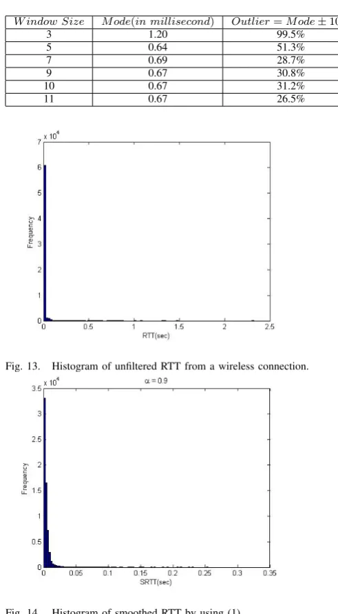
5.2 Unfiltered RTT from a wireless connection. Note that one of the RTT timing is as long as 2.4 seconds. . . 46

(15)

LIST OF FIGURES xiv

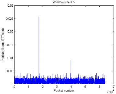
5.4 Median-filtered RTT with window size of five. Only two large RTT’s are not filtered out. . . 47

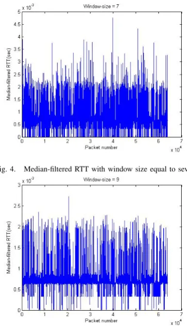
5.5 Median-filtered RTT with window size of seven. There is no significant improvement when the window size is larger than five. . . 47

5.6 Median-filtered RTT with window size of nine. There is no significant improvement when the window size is larger than five. . . 48

5.7 Smoothed RTT by using equation (5.1). The pattern in Figure 5.7 is the same as that in Figure 5.2, except that the amplitude in Figure 5.7 is reduced. . . 50

5.8 Unfiltered RTO from a wireless connection. Figure 5.8 will be compared with other RTO’s in Figure 5.11. . . 52

5.9 Smoothed RTO using (5.2) and (5.3). Figure 5.9 will be compared with other RTO’s in Figure 5.11. . . 52

5.10 Median-filtered RTO with window size of three. Figure 5.10 will be compared with other RTO’s in Figure 5.11. . . 53

5.11 Different RTOs. Median-filtered RTO has amplitude less than those of SRTO and unfiltered RTO. . . 53

5.12 Unfiltered RTO and median-filtered RTO. Median-filtered RTO has am-plitude less than that of unfiltered RTO. . . 54

5.13 Unfiltered RTO and median-filtered RTO (Zoom-in view). Figure 5.13 is the enlargement of Figure 5.12, for the portion near time equal to zero. 54

(16)

LIST OF FIGURES xv

5.15 Histogram of smoothed RTT by using equation (5.1). The RTT’s are distributed in a similar pattern as that in Figure 5.14, except that the

duration is shorter. . . 56

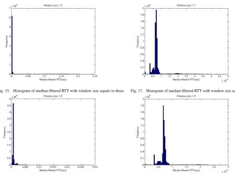
5.16 Histogram of median-filtered RTT with window size of three. For window size of 3, the RTT’s are still distributed on the right side of the mode. It will be seen in later figures that the distribution pattern will change. 56 5.17 Histogram of median-filtered RTT with window size of five. Some RTT’s begin to exist on the left side of the mode. . . 57

5.18 Histogram of median-filtered RTT with window size of seven. The dis-tribution of RTT’s approaches a normal disdis-tribution. . . 57

5.19 Histogram of median-filtered RTT with window size of nine. There are no significant changes after window size of seven. . . 58

5.20 Histogram of median-filtered RTT with window size of eleven. There are no significant changes after window size of seven. . . 58

5.21 Histogram of median-filtered RTT with window size of thirteen. There are no significant changes after window size of seven. . . 59

6.1 Comparison of growth n,nlogn and n2. It can be seen that the growth rate ofn2 is the largest. . . 66

6.2 Experimental results of Shellsort . . . 77

6.3 Experimental results of Quicksort . . . 78

6.4 Experimental results of Fast 1D Median Filtering Algorithm . . . 79

(17)

LIST OF FIGURES xvi

7.1 Simulation Network of Experiment 1, s1 sends packets to d1; s2 to d2 and so on. Links from sources to RO and from R1 to destinations are 10 Mb. ROR1 is a bottleneck of 1 Mb. . . 93

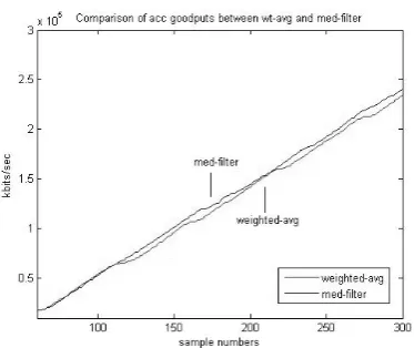
7.2 Comparison of accumulative goodput between median filter and weighted-average filter. This figure shows that a median filter size 5 can deliver higher goodput. . . 94

7.3 RTT and RTO obtained from weighted-average. The RTT curve and RTO curve are farther apart. The response to retransmit when a packet is lost will be too slow. . . 96

7.4 RTT and RTO obtained from median filter of size 5. The RTT curve and RTO curve are closer to each other. This will probably increase the throughput. . . 97

7.5 RTT and RTO obtained from median filter of size 7. Since median filter of size 7 delivers fewer goodput than size 5 does, size 7 is not the best choice. . . 98

7.7 Simulation Network of Experiment 2, s1 sends packets to d1; s2 to d2 and so on. Links from sources to RO and from R1 to destinations are 10 Mb. R0R1 is a bottleneck of 1 Mb. . . 100

7.8 Comparison of accumulative goodput between median filter and weighted-average filter. This figure shows median filter size 5 can deliver more goodput. . . 101

(18)

LIST OF FIGURES xvii

7.10 RTT and RTO obtained from median filter of size 5. . The RTT curve and RTO curve are closer to each other. This will probably increase the throughput. . . 103

7.13 TCP Tahoe throughput versus lossrate. As the lossrate increases, the throughput decreases. . . 107

7.14 TCP Median throughput versus lossrate. As the lossrate increases, the throughput decreases. . . 108

7.15 Throughput of TCP Median decreases to a lesser extent. At high loss rates, there is little to differentiate the two. . . 109

7.16 Throughputs of TCP Tahoe and TCP Median versus packet loss rate. At packet loss rate of 1%, TCP Median outperforms TCP Tahoe by 10%. 111

7.17 Mixed Wireless/Wired Simulation. Packets are sent from S to D via BS. 112

(19)

List of Tables

5.1 Effect on different window sizes . . . 60

6.1 Contributions ofn,nlognand 2n2 to the functiony. It can be seen that 2n2 contributes most toy. . . 65

6.2 Memory Access Analysis on Shellsort main loop . . . 81

6.3 Memory Access Analysis on insertion function . . . 82

6.4 Memory Access Analysis on Quicksort main loop . . . 82

6.5 Memory Access Analysis on partition function . . . 83

6.6 Memory Access Analysis on bubble sort function . . . 85

6.7 Memory Access Analysis on fast median main loop . . . 85

7.1 Exponential traffic and analysis for median filter size 5 and weighted-average filter . . . 95

7.2 Comparison of packet drop percentages. It is found that all packet drop percentages of median filters are lower than that of the weighted-average filter which is 1.66%. . . 99

(20)

LIST OF TABLES xix

(21)

Acronyms & Abbreviations

1D one dimensional

2D two dimensional

ACK Acknowledgement

BIC Binary Increase Congestion Control

CBR Constant Bit Rate

cwnd Congestion window

EWMA Exponential Weighted Moving Average, also called Weighted Average

FIR Finite Impulse Response

FTP File Transfer Protocol IIR Infinite Impulse Response

LAN Local Area Network

Mbps Megabits per second

MF Median Filter

NS2 Network Simulator, version 2 pdf probability density function

RF Radio Frequency

RFC Requests For Comments

RTO Retransmission Timeout

RTT Round Trip Time

ssthresh slow start threshold

tcl Tool Command Language

TCP Transmission Control Protocol

UDP User Datagram Protocol

(22)

Chapter 1

Introduction

1.1

Motivation and Objectives

In wireless networks, electromagnetic waves, instead of cables, are used to connect telecommunication devices such as cellular telephones, communication satellites and wireless local area networks (Goldsmith 2005). The implementation of connecting wire-less networks, take place at the physical layers of the networks (Patil & et al. 2003).

Wireless Local Area Networks use radio frequency (RF) waves to transmit data among computers in a small area such as offices and educational institutions (Goldsmith 2005). Wireless networks are quick-fix methods to connect remote regions, where there is a lack of telecommunications infrastructure, to the Internet. On the other hand, if wired networks are used, long cables are needed to connect these remote regions to the service providers.

Wireless networks are becoming more and more popular. They allow users to access the Internet with their laptop computers at any locations inside their offices or homes, so wireless networks can provide convenience and mobility to their users (Goldsmith 2005).

(23)

1.1 Motivation and Objectives 2

in airports, hotels, cafes and shopping malls to provide wireless access to the Internet for their customers.

In the Internet, reliable data transfer service is provided by Transmission Control Pro-tocol (TCP) (Kurose & Ross 2005). TCP was designed for used in wired network and it does not work so well in wireless networks (Balakrishnan & et al. 1997), because wireless networks have high bit-error rates due to channel fading, noise and interference.

TCP was first proposed for wired networks where packet losses were always due to congestion in the link. Packet losses caused by high bit-error rates in wireless networks, are wrongly interpreted by TCP congestion avoidance algorithm as congestion in the link (Balakrishnan & et al. 1997).

Since TCP was designed originally for wired networks, the motivation of this research project is to investigate the performance of TCP over wireless networks. The main ob-jective of this research project is to enhance TCP performance in managing congestion over wireless networks, by using median filters. Median filters will be used to estimate the Round Trip Time (RTT). Then, the RTT is used to determine the Retransmission Timeout (RTO).

When a host computer sends out a packet, it starts a timer. If the host receives an acknowledgement (ACK) before the timer expires, it sends a new packet and restarts the timer. The time between the stating of the timer and the receiving of ACK is called the Round Trip Time (RTT) (Comer 2006b, Peterson & Davie 2000).

If the timer expires before the host receives an ACK, the host will retransmit the same packet. The time between the starting of the timer and the expiring of the timer is called the Retransmission Timeout (RTO) (Kurose & Ross 2005, Comer 2006b, Peterson & Davie 2000).

(24)

1.2 Organization of this dissertation 3

filter is expected to have a better RTT estimation in such a way that the throughput under bursty traffic increases.

In this research, the median filter is applied to network simulations for retransmission timeout estimation, in the presence of bursty traffic flows. Our simulation results show that, the median filter can perform better than the EWMA filter, in terms of through-put and packet drop percentage, i.e. the median filter delivers more throughthrough-put and loses less packets.

The objectives of this research project are:

1. To review the literature to understand how TCP works. 2. To review the literature to understand median filters.

3. To develop a fast algorithm for median filtering and apply it to the problem of RTT estimation (and hence determination of RTO).

4. To conduct a practical experiment to show that median filter can produce better RTO.

5. Using network simulator version 2 (NS2), to investigate how median filters can improve the retransmission timeout (RTO) of TCP and to use Exponential and Pareto traffic sources in the investigation.

6. To analyse the data obtained in the simulations and to determine whether the median filter can deliver more goodput than weighted-average filter.

7. To present the literature review, practical experiments, NS2 simulations, and analysis of experimental results, in a dissertation.

1.2

Organization of this dissertation

This dissertation is organized as follows:

(25)

1.2 Organization of this dissertation 4

TCP as congestion in the transmission link. How can we improve TCP performance in wireless networks? This question motivated this research project. The objectives of this research project, the dissertation organization, the basic contributions of this research project, and publications generated from this research project are introduced in Chapter 1.

Chapter 2 is a literature review on TCP. The major components of TCP, such as slow start, congestion avoidance, fast retransmit and fast recovery are presented here.

Chapter 3 is a literature review on Round Trip Time and Retransmission Timeout (RTO). The evolution of RTO from its original algorithm to Karn/Partridge algorithm, and then to Jacobson/Karels algorithm are described in this chapter.

Chapter 4 describes the class of median filter algorithms. This chapter includes median filters and some of their modifications. These modifications include ranked-order filters recursive median filters.

In Chapter 5, a practical experiment is presented. There are two approaches to the testing of our median filter algorithm. One approach is by means of practical exper-iment, which is presented in Chapter 5. Another approach is to use software such as Network Simulator, version 2 (NS2) (ISI 2008a) to conduct simulations, which is presented in Chapter 7. In this experiment, a simple point-to-point wireless connec-tion is established between a laptop computer and a desktop computer. Results from the experimental analysis show that median filter algorithm performs better than the weighted-average.

In Chapter 6, the Big-O notation is applied to analyze the speed of the three sorting algorithms. Then, literature reviews on Shellsort and Quicksort are presented. Finally, a fast one-dimensional median filtering algorithm was formulated for TCP, based on the work of T.S. Huanget al..

(26)

1.3 Contributions of this Research Project 5

better than weighted-average filter.

Analysis of simulation results show that median filter delivers more goodput than weighted-average filter does, where goodput is defined as throughput minus retrans-mission. In addition, the median filter has a lower packet drop percentage, meaning that (retransmission/throughput)×100% is lower.

Chapter 8 provides some conclusions on the overall project, and proposes further re-search based on the findings. The primary conclusion is that both practical experiment and simulation show that median filter performs better than EWMA.

1.3

Contributions of this Research Project

The contributions of this research project are briefly presented below:

• The current TCP uses a method called exponential weighted moving average

(EWMA) to estimate the round trip time (RTT). The median filter can perform better than the EWMA. Consistent RTT and smaller retransmission timeout (RTO) are obtained by using median filter. The contribution of this project is that, the above results are desirable factors for higher link throughput.

• A ‘fast’ one-dimensional median filtering algorithm is developed in this project.

Shellsort, Quicksort and the ‘fast’ one-dimensional median filtering algorithms are experimentally used to sort the same set of data, and then the timings, spent by the three methods to sort the same set of data, are compared. Experiments show that the fast one-dimensional median filtering algorithm is faster than Quick-sort and much faster than ShellQuick-sort. The fast one-dimensional median filtering algorithm could satisfy our need of a fast sorting algorithm.

• Simulation results using NS2, with Exponential and Pareto traffics, show that a

(27)

1.4 Further Works of this Research Project 6

1.4

Further Works of this Research Project

The first further development is to improve the computational efficiency of median fil-tering, which involves sorting an array into ascending order and selecting the element at the middle. A decrease in the number of steps in sorting can improve the computa-tional efficiency. For the practical experiment, it should be easy to implement the fast one-dimensional median filtering algorithm developed in this project. For simulation with NS2, it will be a complicated task to modify the program tcp.cc using the fast one-dimensional medium filtering algorithm.

The second further development is to apply median filter in Full TCP. The Tahoe TCP is a one-way agent, which only sends packets from sources to destinations. Full TCP is a two-way agent, which performs bidirectional data transfer. A test can be set up to investigate whether the Full TCP with median filter in it, can deliver more goodput.

(28)

Chapter 2

Transmission Control Protocol

(TCP)

2.1

Introduction

Two researchers, Vinton G. Cerf and Robert E. Kahn, proposed an inter-network pro-tocol called TCP/IP. They published their paper, “A Propro-tocol for Packet Network Intercommunication”, in May 1974 in IEEE Transactions on Communications (Cerf & Kahn 1974).

Current implementations of TCP include four interwoven algorithms as the Internet standards: slow start, congestion avoidance, fast retransmit, and fast recovery. Van Jacobson (Jacobson 1988, Jacobson 1990) provided details on these algorithms. W. Stevens (Stevens 1994) provided examples of the algorithms in action. G. Wright (Stevens & Wright 1995) provided the source codes for the implementation. RFC 1122 requires that a TCP had to implement slow start and congestion avoidance (Braden 1989a), but fast retransmit and fast recovery were implemented after RFC 1122.

(29)

2.2 Slow Start 8

2.2

Slow Start

Slow start is one of the algorithms that TCP uses to control congestion inside the network. It is also known as the exponential growth phase. TCP starts a connection with the sender injecting multiple packets into the network, up to the window size advertised by the receiver. There is no problem when the two hosts are on the same LAN, but if there are routers and slower links between the sender and the receiver, problems can arise. Some intermediate routers must put the packets in queue, and it is possible for these routers to run out of space. The algorithm to avoid this is called slow start. It operates by observing that the rate at which new packets should be injected into the network is the rate at which the acknowledgments (ACKs) are returned by the other end (Jacobson 1988).

Slow start adds another window to the sender’s TCP: the congestion window, abbre-viated to “cwnd”. When a new connection is established by a host on a network, the congestion window is initialized to one packet (i.e., the packet size announced by the other end). Each time an ACK is received, the congestion window is increased by one packet. The sender can transmit up to the minimum of the congestion window and the advertised window. That is, if cwnd is smaller, transmit up to cwnd. If advertised window is smaller, transmit up to advertised window. The congestion window is flow control imposed by the sender, while the advertised window is flow control imposed by the receiver.

The sender starts by transmitting one packet and waits for its ACK. When that ACK is received, the congestion window is increased from one to two, and two packets can be transmitted.

(30)

2.3 Congestion Avoidance 9

Figure 2.1: Packets in transit during slow start

Figure 2.1 shows the growth in the number of packets in transit during slow start, which increases the congestion window exponentially, rather than linearly (Peterson & Davie 2000).

2.3

Congestion Avoidance

Congestion can occur when data arrives on a big pipe (a fast LAN) and it is sent out to a smaller pipe (a slower WAN). Congestion can also occur when multiple input streams arrive at a router whose output capacity is less than the sum of the inputs. Congestion avoidance is a way to deal with lost packets (Braden 1989a).

There are two indications for packet loss: a timeout occurring and the receipt of du-plicate ACKs. Congestion avoidance and slow start are independent algorithms with different objectives. In practice they are implemented together (Jacobson 1988).

(31)

2.4 Fast Retransmit 10

1. Initialization for a given connection sets a slow start threshold, ssthresh, for example, to eight packets, and congestion window, cwnd to one packet.

2. The TCP output routine never sends more than the minimum of cwnd and the receiver’s advertised window.

3. When congestion occurs (indicated by a timeout or the reception of duplicate ACKs), ssthresh is set to one-half of the current window size (the minimum of cwnd and the receiver’s advertised window, but at least two packets). In addition, if the congestion is indicated by a timeout, cwnd is set to one packet (i.e., slow start).

4. When new data is acknowledged by the other end, cwnd is increased, but the way it is increased depends on whether TCP is performing slow start or congestion avoidance.

If cwnd is less than or equal to ssthresh, TCP is in slow start; otherwise TCP is performing congestion avoidance. Slow start continues until TCP reaches ssthresh, and then congestion avoidance takes over.

Slow start has cwnd beginning at one packet, and has cwnd increased by one packet every time an ACK is received. As mentioned earlier, this increases the window expo-nentially: TCP sends one packet, then two, then four, and so on.

Congestion avoidance is a linear growth of cwnd, compared to slow start’s exponential growth. In section 2.6, Illustration of Tahoe and Reno, a graph will be shown to clarify the relationship between slow start and congestion avoidance.

2.4

Fast Retransmit

Modifications to the congestion avoidance algorithm were proposed in 1990 (Jacobson 1990). Researchers realized that TCP generates an immediate acknowledgment (a duplicate ACK) when an out-of-order packet is received. The purpose of this duplicate ACK is to let the other end know that a packet was received out-of-order, and to tell the other end what sequence number is expected (Braden 1989a).

(32)

2.4 Fast Retransmit 11

It is assumed that if there is just a reordering of the packets, there will be only one or two duplicate ACKs before the reordered packet is processed, which will then generate a new ACK. If three or more duplicate ACKs are received in a row, it is a strong indication that a packet has been lost. TCP then performs a retransmission of what appears to be the missing packet, without waiting for a retransmission timer to expire (Stevens 1997). This is called fast retransmit.

Figure 2.2: Fast Retransmit based on duplicate ACKs

(33)

2.5 Fast Recovery 12

2.5

Fast Recovery

When the third duplicate ACK in a row is received, ssthresh is set to one-half the congestion window, the congestion window at the time the third duplicate ACK is received. Then the missing packet is retransmitted (Jacobson 1988).

After fast retransmit sends what appears to be the missing packet, congestion avoid-ance, but not slow start is performed. This is called the fast recovery (Jacobson 1990, Stevens 1994).

In TCP Reno, the fast recovery is implemented but not in TCP Tahoe.

2.6

Illustration of Tahoe and Reno

Figure 2.3: TCP’s congestion window (Tahoe and Reno)

(Kurose & Ross 2005)

(34)

2.7 New Reno TCP 13

hitting the threshold, TCP performs congestion avoidance. The congestion window then climbs linearly until a triple duplicate ACK occurs, just after transmission round 8. The congestion window is 12 packets when this loss event occurs. The new threshold is then set to half congestion window, that is 0.5*12= 6 packets. Under TCP Reno, the congestion window is set to 6 packets (new threshold) and then grows linearly. However, in TCP Tahoe, the congestion window is set to 1 packet and grows exponentially i.e. slow start (Kurose & Ross 2005, Jacobson 1988).

The fast retransmit algorithm first appeared in Tahoe release, and it was followed by slow start. The fast recovery algorithm appeared in Reno release (Stevens 1997, Allman & et al. 1999, Floyd & Henderson 1999).

To sum up, when timeout occurs, both TCP Reno and TCP Tahoe go back to slow start. When three duplicate ACK’s are received, TCP Tahoe performs slow start, but TCP Reno performs congestion avoidance.

2.7

New Reno TCP

New Reno TCP (Floyd & Henderson 1999, Braden & et al. 1998) modifies the action taken when receiving new ACKs. In order to exit fast recovery, the sender must receive an ACK for the highest sequence number sent. Thus, new partial ACKs (those which represent new ACKs but do not represent an ACK of all outstanding data) do not deflate the usable window back to the size of the congestion window.

2.8

Sack TCP

(35)

2.9 Vegas TCP 14

help to overcome these limitations. The receiving TCP sends back SACK packets to the sender informing the sender of the data that has been received. The sender can then retransmit only the missing data packets.

2.9

Vegas TCP

The Vegas extends the Reno’s retransmission mechanisms. At first, Vegas reads and records the system timestamp each time a packet is sent. This is used for following situations (Reddy & Rao 2006):

• When a duplicate acknowledgment is received, Vegas checks to see if the difference

between the current time and the timestamp recorded for the relevant packet is greater than the timeout value. If it is true, then Vegas retransmit the packet without having to wait for duplicate acknowledgments.

• When a non duplicate acknowledgement is received and it is the first or second

one after a retransmission, Vegas checks again to see whether the time interval since the packet is sent, is larger than the timeout value. If it is true that the time interval is larger than the timeout value, then Vegas retransmits the packet.

2.10

BIC and CUBIC TCP

The common concern is that TCP underperforms in those areas of application where there is a high bandwidth-delay system. The problem is that the additive window inflation algorithm used by TCP can be very inefficient in long-delay, high-speed envi-ronments like satellite transmission service.

(36)

2.11 Westwood TCP 15

BIC can be too aggressive in low RTT networks and in slower speed situations, thus leading to a refinement of BIC, namely CUBIC (Rhee & et al. 2008). CUBIC uses a third-order polynomial function to govern the window inflation algorithm, rather than the exponential function used by BIC. CUBIC can produce fairer outcomes in a situation of multiple flows with different RTTs. CUBIC also limits the window adjustment in any single RTT interval to a maximum value.

2.11

Westwood TCP

BIC and CUBIC concentrate on the rate increase function, attempting to provide for greater stability for TCP sessions as they converge to a long-term available sending rate. The other perspective is to examine the multiplicative decrease function, to see if there is further information that a TCP session can use to modify this rate decrease function (Huston 2006).

(37)

2.12 TCP Evolution 16

2.12

TCP Evolution

The evolution of TCP is to seek a point of delicate balance between self-optimization and cooperative behavior. Self-optimization is to optimize the use of bandwidth for one of the users in the link, while cooperative behavior is to consider the need of other users in the link and to give a fair share of the bandwidth of the link to other users.

The evolution of TCP must avoid making radical changes that may stress the deployed network into congestion collapse, and also must avoid a congestion control among com-peting protocols (Gerla & et al. 2001). The Internet architecture to date has been able to achieve new benchmarks of network efficiency. Much of the credit for this must go to the operation of TCP, which manages to work at that point of delicate balance between self-optimization and cooperative behavior.

Widespread deployment of transmission protocols that take a more aggressive position on self-optimization will ultimately lead to situations of congestion collapse. On the other hand, widespread deployment of conservative transmission protocols may lead to lower jitter and lower packet retransmission rates, but at a cost of considerably lower network efficiency (Floyd 2000).

The challenges faced with the evolution of TCP is to maintain a coherent control architecture that has consistent behavior within the network, consistent interaction with instances of data flows that use the same control architecture, but adequately flexible to adapt to differing network characteristics and different application profiles (Huston 2000).

2.13

Summary

(38)

2.13 Summary 17

Upon receiving three duplicate ACK’s, Tahoe TCP retransmits the packet that appears to be lost, without waiting for the retransmission timer to expire. This is the fast retransmit algorithm.

Reno TCP includes fast recovery. In addition, Reno TCP does not return to slow start during fast retransmit, but reduces the congestion window to half its current value.

Each variation of TCP is designed to solve a special problem using a specific method, and is suitable for a particular application. For instance, Binary Increase Congestion Control TCP (BIC TCP) searches for a packet sending rate that is on the threshold of triggering packet loss, and uses a binary search algorithm to achieve this. BIC TCP is designed for use in long-delay, high speed environments like satellite transmission service.

In the next chapter, Round Trip Time (RTT) and Retransmission Timeout (RTO) and Jacobson/Karels Algorithm will be introduced. All these topics are closely related to TCP.

(39)

Chapter 3

Round Trip Time (RTT) and

Retransmission Timeout (RTO)

3.1

Introduction

When timeout occurs, both TCP Reno and TCP Tahoe return to slow start, as men-tioned in Section 2.6. At slow start, TCP begins transmission with one packet. It is obvious that the value of timeout affects the throughput of the transmission link. This chapter presents an in-depth review of retransmission timeout.

The reliability of delivery of data is guaranteed in Transmission Control Protocol (TCP) by the following procedure. When a host computer sends a packet, it starts a timer. If the host receives an acknowledgement (ACK) before the timer expires, it sends a new packet and restarts the timer. The time between the starting of the timer and the receiving of ACK is called the Round Trip Time (RTT) (Comer 2006a, Peterson & Davie 2000).

(40)

3.2 Historical Development of RTO 19

It is obvious that the RTO should be larger than the RTT; but how much larger should RTO be (Comer 2006a)? The answer to this question is the focus of this project.

This chapter starts with highlighting the difficulties in choosing RTO. Three algorithms are presented for the estimation of RTO, namely: the Original Algorithm specified by RFC 793 in 1981 (Postel 1981), the Karn/Partridge Algorithm specified by the publication, “Improving Round-Trip-Time Estimates in Reliable Transport Protocols”, in 1987 (Karn & Partridge 1995); and the Jacobson/Karels Algorithm specified by the paper “Congestion Avoidance and Control” published in 1988 (Jacobson 1988). Then there is a section on the historical development of RTO. Finally, Exponential distribution and Pareto distribution are introduced.

3.2

Historical Development of RTO

Retransmission timeout (RTO) estimation is important for data transmission in the Internet so it is worthwhile to investigate the historical development of RTO and the problems involved in RTT estimation.

The TCP specification that specifies the first original algorithm (Section 3.4), is RFC 793, which was published in 1981 (Postel 1981).

The first original algorithm, after several years of implementation in the Internet, was found to have ambiguity in the measurement of RTTs that were retransmitted (Section 3.5).

In 1987, Phil Karn of Bell Communication Research, and Craig Partridge of Harvard University, found that TCP was suffering from a problem they called retransmission ambiguity.

(41)

3.3 Difficulties in Choosing RTO 20

Internet more effectively.

At the time RFC 793 and clarification of retransmission ambiguity were implemented in the Internet, TCP used window based flow control, as a means for the receiver to restrict the amount of data sent by the sender. This flow control was used to prevent overflow of the receiver’s data buffer, available for that connection. TCP assumes that packets could be lost due to either errors or congestion, but did not implement any dynamic mechanism to adjust the flow control window in response to congestion.

In October, 1986, Van Jacobson reported the first Internet congestion collapse. The data throughput from Lawrence Berkeley Laboratory to University of California Berke-ley, which are 400 yards (1 yard = 0.92 meter) apart, dropped from 32 Kbps to 40 bps. Van Jacobson and Mike Karels started to investigate why the drop was so big (Jacobson 1988).

In 1988, Van Jacobson published his paper, “Congestion Avoidance and Control”, (Jacobson 1988). Although the paper was published under the name of Van Jacobson, Jacobson acknowledged in his paper that the algorithms and ideas described in his paper were developed in collaboration with Mike Karels of University of California Berkeley, Computer System Research Group.

In his paper, Jacobson presented the Jacobson/Karels Algorithm which was described in Section 3.6, in addition to slow-start, congestion avoidance, and fast retransmit.

Slow-start, congestion avoidance and fast retransmit were described in Chapter 2, and Jacobson/Karels Algorithm was described in Chapter 3. These descriptions give the impression that Chapter 2 and Chapter 3 are separate issues. It should be pointed out that Chapter 2 and Chapter 3 are related issues. They are presented in two separate chapters for the reason of easy understanding.

3.3

Difficulties in Choosing RTO

(42)

3.4 Original Algorithm 21

• The range of variation in RTTs between two host computers is great (Peterson

& Davie 2000);

• If RTO is just a little larger than RTT, retransmission will be too often, and that

increases congestion in the transmission path (Comer 2006a);

• If RTO is much larger than RTT, the response to retransmit when a packet is

lost, will be too slow; and this will decrease the throughput of the transmission path (Comer 2006a).

The RTO now implemented in TCP was proposed by Jacobson in 1988 (Comer 2006a, Peterson & Davie 2000); but before this Jacobson/Karels algorithm, there were the original algorithm and Karn/Partridge algorithm. These three algorithms are described in the following sections in chronological order.

3.4

Original Algorithm

This section presents the first original algorithm prescribed in the TCP specification (Peterson & Davie 2000). When TCP sends a packet, it starts a timer. When an ACK of that packet is received, TCP stops the timer and reads the time, which is taken to be the Sample RTT. A new Estimated RTT is the weighted average of the old Estimated RTT and the Sample RTT. Expressing the above idea in formula:

Ai = (1−G1)Ai−1+G1Mi−1 (3.1) where Ai is the new Estimated RTT;

Ai−1 is the old Estimated RTT; Mi−1 is the Sample RTT.

G1 is a constant, which is typically equal to 0.125. (0.125=1/8). Therefore,

New Estimated RTT = (0.875)(Old Estimated RTT) + (0.125)(Sample RTT) The RTO is then calculated by the simple formula

(43)

3.5 Karn/Partridge Algorithm 22

The first original specification recommendedβ = 2.

References for the above formulas are from RFC 793.

3.5

Karn/Partridge Algorithm

The first original algorithm, after several years of implementation in the Internet, was found to be inadequate. Problems arose when there was retransmission.

When a packet was retransmitted and then an ACK was received, it was impossible to know whether this ACK was associated with the original transmission or the retrans-mission.

Figure 3.1: ACK for retransmission

In Figure 3.1,A represents original transmission; B represents retransmission; C

(44)

3.5 Karn/Partridge Algorithm 23

Figure 3.2: ACK for original transmission

In Figure 3.2,Arepresents original transmission;Brepresents retransmission;C

repre-sents ACK. If it was assumed that the ACK was for retransmission, but it was actually for the original transmission as shown in Figure 3.2, then the calculated Sample RTT would be too small (Kurose & Ross 2005, Peterson & Davie 2000).

In 1987, Karn and Partridge proposed the Karn/Partridge algorithm, which is described below:

• TCP calculated Sample RTT only for packets that were sent once, and did not

calculate Sample RTT for packets that were sent twice, that is, for packets that were retransmitted (Kurose & Ross 2005, Peterson & Davie 2000).

• Whenever there was retransmission, TCP used the following formula to calculate

RTO:

Ri= (2)(Ri−1) (3.3)

Ri Next retransmission timeout

Ri−1 Last retransmission timeout

(45)

3.6 Jacobson/Karels Algorithm 24

3.6

Jacobson/Karels Algorithm

In 1988, two researchers, Jacobson and Karels, proposed their Jacobson / Karels Al-gorithm (Comer 2006a, Peterson & Davie 2000), which is described by the following formulas (3.4), (3.5), (3.6), (3.7):

Firstly, find the difference between the Sample RTT and the old Estimated RTT.

Difference =Mi−1−Ai−1 (3.4)

where Mi−1 is the Sample RTT (Kurose & Ross 2005, Peterson & Davie 2000). Secondly, find the new Estimated RTT by Equation (3.5).

Ai=Ai−1+ (G1)(Difference) =Ai−1+ (G1)(Mi−1−Ai−1) =Ai−1+G1Mi−1−G1Ai−1 = (1−G1)Ai−1+G1Mi−1

(3.5)

G1 is a constant, which is typically equal to 0.125 (Kurose & Ross 2005, Peterson & Davie 2000, Ma & et al. 2004). (0.125=1/8) The Ai described in this section is the

same as that presented in Original Algorithm. Thirdly, find the new deviation from the old deviation by Equation (3.6).

(3.6)

where Vi is the new deviation;

Vi−1 is the old deviation;

|Difference|is absolute value of Difference;

G2 is a constant, which is typically equal to 0.25 . (0.25=1/4) (Kurose & Ross 2005, Peterson & Davie 2000, Ma & et al. 2004)

Finally, find the next retransmission timeout from the new Estimated RTT and new deviation.

(46)

3.7 More about Jacobson/Karels Algorithm 25

where Ri is the next retransmission timeout;

Vi is the new deviation

K is a constant, which is typically equal to 4.

(Kurose & Ross 2005, Peterson & Davie 2000, Ma & et al. 2004)

3.7

More about Jacobson/Karels Algorithm

Jacobson performed a practical experiment, and plotted RTT and RTO in the same figure, in order to prove that his Algorithm is superior to RFC 793.

Figure 3.3: RTO computed by RFC 793 rules (Jacobson 1988)

(47)

3.7 More about Jacobson/Karels Algorithm 26

The dotted line shows the RTTs. The solid line shows the RTOs computed according to the rules of RFC 793 (Jacobson 1988).

Figure 3.4: RTO computed by Jacobson/Karels Algorithm (Jacobson 1988)

Figure 3.4 shows the same data as above, but the solid line shows RTOs computed according to Jacobson/Karels Algorithm (Jacobson 1988).

When Figure 3.3 and Figure 3.4 are compared, it is found that the shape of the solid line in Figure 3.4 resembles the shape of the dotted line. Also, the solid line of RTOs is closer to the dotted line of RTTs.

In Chapter 7, simulations of TCP using median filter are conducted. By plotting RTTs and RTOs in the same figure, RTTs and RTOs resemblance in shapes, and closeness in lines. Our simulations in Chapter 7 are supported by Figure 3.3 and Figure 3.4.

(48)

3.8 Problems with RTT Estimation 27

RTO = (new Estimated RTT) + (4)(new deviation)]

In a 9.6 kb link, the link utilization could go from 10% to 90% as a result of imple-menting Jacobson/Karels Algorithm (Braden 1989b).

For a new connection, the initializations should be: RTT = 0 second

RTO = 3 seconds

The lower bound for RTO should be in fractions of a second (to accommodate high speed LANs), and the upper bound should be 240 seconds (Braden 1989b).

Jacobson and Karels made a great contribution to prevent congestion collapse in today’s Internet.

3.8

Problems with RTT Estimation

The first problem with RTT estimation is described as follows: RFC 793 suggested finding:

New Estimated RTT = (7/8)(Old Estimated RTT) + (1/8)(Sample RTT) and then calculated

RTO = (β)(New Estimated RTT).

The suggestedβ=2 could adapt to loads of at most 30% (Jacobson 1988). Above this

point, a connection would respond to load increases by retransmitting packets that had only been delayed in transit (Jacobson 1988). This would cause a more serious congestion in the network.

There is still another problem to be discussed below:

Ai = (1−G1)Ai−1+G1Mi−1

Mi−1 Sample RTT

(49)

3.9 Exponential Distribution and Pareto Distribution 28

Ai =Ai−1−G1Ai−1+G1Mi−1

Ai =Ai−1+G1(Mi−1−Ai−1)

The last expression above states that a new prediction (Ai) is made, based on the old

prediction (Ai−1), plus a fraction (G1=1/8) of the prediction error (Mi−1−Ai−1).

The prediction error is the sum of two components:

1. Error due to noise in the measurement, which is random and unpredictable, such as fluctuations in competing traffic. This part is denoted byEr.

2. Error due to a poor choice ofAi−1. This part is denoted by Ee.

Then Ai=Ai−1+G1Er+G1Ee

The G1Ee term moves Ai in the correct direction while G1Er moves Ai in a random

direction (Jacobson 1988).

IfAifollows a Gaussian distribution (also called normal distribution),G1Er will cancel

one another after a number of samples, and Ai will converge to the correct value.

Unfortunately,Aidoes not follow a Gaussian distribution. Instead,Ai follows a

heavy-tailed distribution.

3.9

Exponential Distribution and Pareto Distribution

In 1995, two researchers Paxson and Floyd found that FTP data connections had bursty arrival rates. In addition, the distribution of the number of bytes in each burst has a heavy right tail (Paxson & Floyd 1994).

In statistics, heavy-tailed distributions are probability distributions whose tails are not exponentially bounded (Asmussen 2003). That is, they have heavier tails than the exponential distribution.

(50)

Since exponential and Pareto traffics will be used in Chapter 7 simulations, it is neces-sary to understand their pdf’s.

Exponential distribution (Drossman & Veirs 2002) is defined as:

N(x) =              N0

eαx forx >0

0 elsewhere

(3.8)

In order to see the similarity between Exponential distribution and Pareto distribution, N(x) is simplified as follows:

Letα = 1.

Then,N(x) = N0

2.7x whereN0, the value of N(x) at time x = 0, is a constant. Later, it will be shown that one example of Pareto distribution is : f(x) = Constant_x2.7

Now Pareto distribution will be introduced. The definition of Pareto distribution (Freund & Walpole 1987) is:

f(x) =              αkα

xα+1 forx >k

0 elsewhere

(3.9)

Let us consider the simple case where k = 1.

f(x) =              α

xα+1 forx >1

0 elsewhere

(3.10)

Letα = 1.7 f(x) = _x12.7.7

There is similarity between exponential distribution and Pareto distribution. The pa-rameter k specifies the minimum value of x. The papa-rameterα determines the shape of

(51)

Exponential distribution and Pareto distribution in Figure 3.5 are plotted for compar-ison. In Figure 3.5, Pareto distribution decreases much more slowly than exponential

Figure 3.5: Exponential and Pareto probability density functions (Hei 2001)

distribution. In other words, Pareto distribution has a heavier tail than exponential distribution.

In 1997, Willingeret al. (Willinger & et al. 1997) generated Ethernet traffic by super-position of many Pareto traffic sources, setting them ON and OFF. During ON period, the source transmits a burst of packets. During OFF period, the source is in idle and no packets are transmitted.

In Chapter 7, the ON period, OFF period and shape of the Pareto traffic are set in our simulations.

(52)

3.10 Summary 31

3.10

Summary

This chapter builds up theoretical foundations to support our network simulations in Chapter 7. In Section 3.4, the original algorithm states that a new Estimated RTT is the weighted average of the old Estimated RTT and the Sample RTT. The RTO is then calculated as two times new Estimated RTT. Our proposal in Chapter 7 is that, a new Estimated RTT is the median of the latest five Sample RTT’s; and the RTO is then calculated as 1.25 times new Estimated RTT. What will be done in Chapter 7, is to replace weighted-average filter with median filter.

Jacobson had performed a practical experiment, and plotted RTT and RTO in the same figure to show that his algorithm is superior to RFC 793 (Refer to Section 3.2). This idea will be used to plot RTT and RTO in the same figure, to show that our proposal of using median filter, is better than weighted-average filter in Chapter 7.

(53)

Chapter 4

The Median Filter and its

Modifications

4.1

Introduction

Since one of the objectives of this project is to apply the median filter to find a better round trip time (RTT), it is appropriate to review some literature on these topics. A literature review of these topics is presented below. Linear filter does not preserve sharp edges of signals well (Yin & et al. 1996), and it cannot attenuate impulsive noise totally. The nonlinear median filter can overcome these two problems; it can preserve sharp edges and at the same time, attenuate impulsive noise very well (Nodes & Gallagher Jr. 1982).

Topics presented in the following sections are:

• Median Filters

• Ranked-order Filters

• Recursive Median Filters

• Weighted Median Filters

(54)

4.2 Median Filter 33

• Symmetric Weighted Median Filters

• Centre Weighted Median Filters

• Adaptive Weighted Median Filters

4.2

Median Filter

Median Filter was proposed by J. Tukey in 1974 (Tukey 1974). It is a nonlinear filter and the principle of superposition that applies to linear filter does not apply to it (Yin & et al. 1996). An array is input to the median filter. The input array is sorted either in ascending or descending order. The output of the median filter is the middle element of the sorted input array.

Properties of Median Filters

Signals invariant to further median filtering is called the root signal (Arce & Gallagher Jr. 1982).

A finite number of repeated median filtering of a signal of finite length will yield a root signal (Yin & et al. 1996). This property of median filters is called the convergence property.

A root signal remains unchanged after further median filtering (Burian & Kuosmanen 2002). A root signal of a median filter of length 2k+1, is also a root signal of median filter of length less than2k+1 (Nodes & Gallagher Jr. 1982).

For a median filter of length2k+1,

X₍_n₎=medianhX₍_n₋_k₎,_{· · ·}, Xn,· · ·, X(n+k) i

(4.1)

X₍_n₎ is called the root signal of that particular median filter, if the above condition is

satisfied for all n (Yin & et al. 1996, Mitra & Kaiser 1993). The two important properties of the median filter are: (a) edge preservation,

(55)

4.2 Median Filter 34

Since impulse has high frequency content, and median filter attenuates it, median filter is a low-pass filter (Arce & Stevenson 1987).

Figure 4.1: Median Filters suppress impulse and at the same time preserve edge (Mitra & Kaiser 1993)

In digital image processing, positive and negative impulses appear in the photograph as white and black dots (or black and white dots). This impulsive noise is given the namesalt and pepper noisebecause salt is white and pepper is black in colour.

Salt and pepper noise can be removed by using median filter.

Example for Median Filter (Pratt 1978):

Apply median filter with window size of 3 to the arrayx(n), wherex(n) = [2 80 6 3].

Solution

y[1] = Median [2 2 80] = 2

y[2] = Median [2 80 6] = Median [2 6 80] = 6 y[3] = Median [80 6 3] = Median [3 6 80] = 6 y[4] = Median [6 3 3] = Median [3 3 6] = 3

(56)

4.3 Ranked-order Filters 35

Some concepts presented by Gallapher and Wise (Gallagher Jr. & Wise 1981) related to root signals are summarized below:

For a median filter of length2k+1,

• a constant neighbourhood is a region of at leastk+1 consecutive identically valued points (Gallagher Jr. & Wise 1981);

• an edge is a monotonically rising or falling set of points surrounded on both sides

by constant neighbourhoods of different values (Gallagher Jr. & Wise 1981);

• an impulse is a set of at least one but less than k+1 points (in other words, an impulse is a set of at least one and at mostk points), whose values are different from the surrounding regions, which are identically valued constant neighbour-hoods (Gallagher Jr. & Wise 1981);

• an oscillation is any signal structure that is not part of a constant neighbourhood,

an edge or an impulse (Gallagher Jr. & Wise 1981).

4.3

Ranked-order Filters

The ranked-order filter was first introduced by Arce and Stevenson in 1987. It takes the i-th largest sample from the input data set, as its output. Y(n) = i-th largest value of the set [X₍_n₋_k₎, ..., X₍_n₎, ..., X₍_n₊_k₎] whereY₍_n₎ is the output, andX₍_n₎’s are the inputs

(Yin & et al. 1996).

Maximum filter and minimum filter are two special cases of ranked-order filter. Max-imum filter and minMax-imum filter take the maxMax-imum sample and the minMax-imum sample from the input data set, as their outputs respectively (Yin & et al. 1996).

(57)

4.4 Recursive Median Filters 36

Example for Ranked-order Filter (Poularikas 1999):

Given input data set X = [4,14,18,40,10] Find the outputs of the ranked-order filter.

SolutionSort X and store inX-ordered. X-ordered = [4, 10, 14, 18, 40]

Forrank r = 1, the output = 4. Forrank r = 2, the output = 10.

Forrank r = 3, the output = 14 = median Forrank r = 4, the output = 18.

Forrank r = 5, the output = 40.

4.4

Recursive Median Filters

Recursive median filter is a modification of median filter. It uses the previously derived output samples to replace some of the input samples. A recursive median filter of length 2k+1 is defined by the following equation (Yin & et al. 1996, Mitra & Kaiser 1993):

Y₍_n₎ =medianhY₍_n₋_k₎,_{· · ·}, Y₍_n₋₁₎, Xn, X(n+1),· · ·, X(n+k) i

(4.2)

where Ynis output;

Y₍_n₋_k₎,_{· · ·}, Y₍_n₋₁₎ are the previous output samples; X(n), X(n+1),· · ·, X(n+k) are the input samples. Recursive median filtering is carried out in two steps.

• The previously derived output is used to replace the old input.

• Then the window of the recursive filter is moved to the next position (Yin &

(58)

4.5 Weighted Median Filters 37

4.4.1 Properties of Recursive Median Filter

For the same number of filtering operations, the recursive median filter provides better smoothing effect than the original median filter, but the input signal is distorted more after recursive median filtering (Yin & et al. 1996, Burian & Kuosmanen 2002).

If a median filter can produce a root signal after one filtering, the median filter is said to be idempotent (Haavisto & et al. 1991). One recursive median filtering operation will cause an input signal to become the root signal (Mitra & Kaiser 1993). The recursive median filter is described as idempotent for possessing this ability (Yin & et al. 1996, Burian & Kuosmanen 2002). Recursive median filter is idempotent when filtering one-dimensional signals, but this is not generally true for two-dimensional signals.

Repeated non-recursive median filtering operations also cause an input signal to become the root signal. However, the root signals produced by non-recursive and recursive operations are generally not the same (Yin & et al. 1996, Mitra & Kaiser 1993, Burian & Kuosmanen 2002).

4.5

Weighted Median Filters

When a particular element in the input array is more important than the other elements, it is duplicated in the input array. The number of times for which it is duplicated is called the weight of that particular element. For example, in the input array of [1, 2, 3, 4, 5], the element 2 is more important. It is duplicated three times to reflect its importance. The array then becomes [1, 2, 2, 2, 3, 4, 5]. The weight of 2 is said to be three.

(59)

4.5 Weighted Median Filters 38

The first definition of weighted median filter is stated below (Yin & et al. 1996, Mitra & Kaiser 1993):

LetX = [X1,X2,· · ·,XN] be a discrete-time continuous-valued input vector,

W = [W1,W2,· · ·,WN] be the integer weights. Then the output

Y=median[W1♦X1, W2♦X2,· · ·, WN♦XN] (4.3)

where the♦ denotes duplication, that is,

A♦X=X,· · ·, X | {z } A times

(4.4)

The second definition of weighted median of X is stated as follows: The weighted median isβ that minimizes the sum

N

X

i=1

W_i|Xi−β| (4.5)

where Xi and Wi are defined as in the first definition (Yin & et al. 1996, Mitra &

Kaiser 1993). β is chosen from X.

Example of Weighted Median Filter (Poularikas 1999):

Given the input vectorX = [4, 14, 18, 40, 10] and the weight W= [-0.05, 0.1, 0.15, 0.1, 0.05] find the output of the weighted median filter.

Solution

PutX and W in small brackets and store inY.

Y = [(4, -0.05), (14, 0.1), (18, 0.15), (40, 0.1), (10, 0.05)] Move the negative sign in weight to input data.

Y = [(-4, 0.05), (14, 0.1), (18, 0.15), (40, 0.1), (10, 0.05)] SortY according to X and store inZ.

Z= [(-4, 0.05), (10, 0.05), (14, 0.1), (18, 0.15), (40, 0.1)] Find the sum of weight and then divide it by two.

(60)

4.6 Recursive Weighted Median Filters (RWMF) 39

Add the weights 0.05 + 0.05 + 0.1 +0.15 = 0.35 until the sum of the weights is larger than the halfsum. The last weight 0.15 belongs to 18, so 18 is the weighted median filter output.

4.6

Recursive Weighted Median Filters (RWMF)

The recursive weighted median filter is obtained by combining the recursive median filter and weighted median filter.

When filtering one-dimensional signals, RWMF is usually not idempotent (Burian & Kuosmanen 2002). RWMF is better than Infinite Impulse Response (IIR) filter be-cause bandpass RWMF and highpass RWMF can be designed to have good stopband characteristics which IIR cannot attain (Arce & Paredes 2000).

RWMF is similar to IIR filter in structure (Arce & Paredes 2000). The difference equation of IIR filter is stated below:

Y(n) =

N

X

l=1

AlY(n−l) + q

X

k=−p

BkX(n−k) (4.6)

where Y(n) is the output;

Y(n−l) is the previous output; X(n₋k) is the input;

Al is the weight called feedback coefficient; and

Bk is the weight called feedforward coefficient.

A total of (N+p+q+1) coefficient is needed to define the recursive difference equation. The following replacements can be used to obtain the RWMF (Arce & Paredes 2000).

• Replace summation sign by median operation.

• Replace multiplication weighting by signed duplication weighting.

(61)

4.7 Symmetric Weighted Median Filters 40

Paredes 2000):

Y(n) =median 

_|Al|♦sgn(Al)Y(n−l)

N l=1

+|Bk|♦sgn(Bk)X(n−k)

q

k=−p



 (4.7)

wheresgn denotes the sign function defined as: sgn(X) = +1 if X_≥0

sgn(X) = ₋1 if X<0

Example:

GivenY(n) =median[Y(n₋1), X(n), X(n+ 1), X(n+ 2), X(n+ 3)]

Y(n) Output

Y(n−1) Previous output

X(n), X(n+ 1), X(n+ 2), X(n+ 3) Input samples

and givenY(n) =median[4,14,18,40,10],

and given weightW= [₋0.05,0.1,0.15,0.1,0.05],

find the outputY(n).

Solution

The answer is the same as that given in weighted median filter, soY(n)=18.

The only difference is that the first data Y(n₋1), which is 4, comes from previous

output.

4.7

Symmetric Weighted Median Filters

A weighted median filter is symmetric if the integer weights

W =hW₋N· · ·, W−1, W0, W1· · ·, WN

i

is symmetric (Yin & et al. 1996). (4.8)

(62)

4.8 Centre Weighted Median Filters (CWMF) 41

4.8

Centre Weighted Median Filters (CWMF)

In centre weighted median filter, weight is only assigned to the centre input sample, and not to the rest of the input samples (Yin & et al. 1996).

In other words, only the centre sample has a weight larger than one and all other samples have weights equal to one (Burian & Kuosmanen 2002).

CWMF is specified by its filter length and centre weight, and it can be designed to possess good noise attenuation while preserving details of the original image (Burian & Kuosmanen 2002).

4.9

Adaptive Weighted Median Filters

In digital image processing, the weights in weighted median filter are assigned as a compromise between edge preservation and noise attenuation. Thus, weighted median filter is optimum for the whole image but not for local areas. A solution to overcome this drawback of weighted median filter is to assign adaptive weights according to local characteristics of the image. It is possible to design an adaptive weighted median filter whose weights change according to the local characteristics of the image, so that both maximum noise attenuation and maximum edge preservation can be achieved (Meguro & Taguchi 1996).

When an adaptive weighted median filter is applied to a particular situation, the weights can be changed according to that special application.

A simple example of adaptive weighted median filter is given here.

In this simple example of adaptive weighted median filter, weights are assigned accord-ing to the followaccord-ing rules:

• Weight is assigned only to the immediate input sample Ik, while keeping the

(63)

4.9 Adaptive Weighted Median Filters 42

• The value of the weight assigned to Ik, depends on the rank of the sample Ik,

among all other samples, which are all inside the observation window (Ma & et al. 2003).

The weightw of Ik is assigned by the rule:

w=L+ 1₋rk (4.9)

where L is the number of samples inside the observation window (i.e. there are L

samples);rk is the rank of the sample Ik.

Case 1:

If there are 7 samples, thenL= 7.

IfIk, is ranked 1, then rk = 1.

w= 7 + 1 - 1 = 7

The weight assigned toIk is 7.

Case 2:

IfL is still 7, andIk is ranked 7, and therefore rk = 7.

w= 7 + 1 - 7 w= 1

In this case, the weight assigned to Ik is 1, so the adaptive weighted median filter is

reduced to median filter.

The above adaptive weighted median filter can be applied to Random Early Drop gateway (Floyd & Jacobson 1993).

Example 1:

If the immediate queue size Ik of the gateway is the smallest inside the observation

window, this can be interpreted as no congestion. By following this trend, the largest possible weight is assigned toIk.

If the queue sizes are sorted in ascending order, with the smallest sample being put on the left and the largest sample being put on the right, then the rankrk of Ik is 1.

w=L+ 1₋rk

(64)

4.10 Summary 43

In this way, when Ik is the smallest, it is assigned the largest weight L. For example,

if there are totally 7 samples, the weight assigned is 7.

Example 2:

Next, suppose the immediate queue size Ik of the gateway is the largest inside the

observation window, it is interpreted as congestion. This time, the trend will not be followed. The

Improving wireless TCP/IP performance using the median filter algorithm

University of Southern Queensland

Associated Publications

Acknowledgments

Contents

List of Figures

List of Tables

Acronyms & Abbreviations

Chapter 1

Organization of this dissertation

Contributions of this Research Project

Further Works of this Research Project

Introduction

Slow Start

Congestion Avoidance

Fast Retransmit

Fast Recovery

Illustration of Tahoe and Reno

New Reno TCP

Vegas TCP

BIC and CUBIC TCP

Westwood TCP

Summary

Chapter 3

Historical Development of RTO

Difficulties in Choosing RTO

Original Algorithm

Karn/Partridge Algorithm

Jacobson/Karels Algorithm

More about Jacobson/Karels Algorithm

Problems with RTT Estimation

Exponential Distribution and Pareto Distribution

Summary

Modifications

Median Filter

Ranked-order Filters

Recursive Median Filters

Weighted Median Filters

Recursive Weighted Median Filters (RWMF)

Symmetric Weighted Median Filters

Adaptive Weighted Median Filters