Chapter 3
Ocean model spin-up
procedures
3.1
Introduction
The control climates of the Mk3L atmosphere and ocean models were evaluated in Chapter 2. A number of deficiencies were noted, including that:
• The climate of the ocean model is only moderately realistic. The deep ocean is too cold, too fresh and too buoyant, and the rate of North Atlantic Deep Water formation is too weak.
• There are significant mismatches between the surface fluxes diagnosed from the atmosphere and ocean model spin-up runs. In some regions, these mismatches are larger in magnitude than the fluxes themselves.
The deficiencies in the climate of the ocean model arise, in part, because the surface waters in the regions of deep water formation are insufficiently dense or saline (England and Hirst, 1997; Bi, 2002). While this may indicate deficiencies in the model physics, an alternative explanation is associated with the surface boundary conditions on the ocean model. These have two potential flaws:
• The relaxation boundary condition is physically unrealistic, and ensures that the peak winter density and salinity of the surface waters do not attain the maximum observed values (England and Hirst, 1997; Bi, 2002).
• The prescribed sea surface temperatures and salinities may be erroneous. In particular, a “fair weather” bias in observed sea surface temperatures and salinities at high latitudes, including a lack of observations beneath sea ice, has been noted (e.g.Weaver and Hughes, 1996;Duffy and Caldeira, 1997). As a result of this bias, the observed sea surface temperatures can be too high, and the sea surface salinities too low.
In Section 3.2, the surface boundary conditions which have been employed in other studies are examined. It is concluded that the relaxation boundary condition is
the most appropriate, as it gives rise to a stable ocean climate. The default response of the Mk3L ocean model to the relaxation boundary condition is therefore studied in further detail in Section 3.3.
Potential modifications to the relaxation boundary condition are considered in Section 3.4. The remainder of the chapter then studies the dependence of the simu-lated ocean climate upon the relaxation timescale. In Section 3.5, this relationship is investigated using a simple theoretical slab ocean model. In Section 3.6, a series of spin-up runs are then conducted using the Mk3L ocean model, with the relaxation timescale being varied from 5 to 80 days.
The dependence of the simulated ocean climate upon the prescribed sea surface temperatures and salinities is studied in Chapter 4.
3.2
Surface boundary conditions
3.2.1 The relaxation boundary condition
Under the relaxation boundary condition on the sea surface temperature (SST) and sea surface salinity (SSS), the temperature and salinity of the upper level of the ocean model are relaxed towards prescribed values. An exponential relaxation is employed, using a constant timescale.
The Mk3L ocean model uses the relaxation boundary condition to calculate the surface heat flux F and the surface salinity tendencydSO/dt as follows:
F = cv∆z γ(Tobs−T) (3.1)
dSO
dt = γ(Sobs−S) (3.2)
Here, T and S are the temperature and salinity, respectively, of the upper level of the model, Tobs and Sobs are the prescribed SST and SSS respectively, cv is the
volumetric heat capacity of seawater, and ∆z is the thickness of the upper layer of the ocean model. γ is the relaxation constant, and is equal to the inverse of the relaxation timescale. The model employs an insulating boundary condition at lateral walls and at the base; neither are there any internal sources of heat or salt. The evolution of the heat and salt contents of the ocean are therefore governed entirely by the respective surface fluxes, and by internal redistribution of these properties.
From Equations 3.1 and 3.2, it can be seen that the surface fluxes are linearly proportional to the difference between the prescribed and simulated values for the surface tracers. The constants of proportionality arecv∆z γ for the SST, andγ for
the SSS; for a relaxation timescale of 20 days, these equate to ∼59 Wm−2K−1 and ∼5.8×10⁻⁷ s−1 respectively.
The prescribed SST and SSS for spin-up run O-DEF (Section 2.3.2) were taken from the World Ocean Atlas 1998 (National Oceanographic Data Center, 2002). However, the use of observational values for the prescribed SST and SSS precludes the possibility that the simulated SST and SSS can equal the observed values, and
3.2. SURFACE BOUNDARY CONDITIONS 59
conjunction with observational values for the SST and SSS therefore ensures that there must be discrepancies in the ocean model climate. An alternative approach to the relaxation boundary condition on the SST is that of Haney (1971) and Han
(1984), in which Tobs in Equation 3.1 is set equal to a prescribed apparent surface air temperature. These temperatures are calculated such that, when the simulated SST is equal to an observed value, the surface heat flux will also be equal to an observed value.
The relaxation boundary condition on the SST simulates the strong feedback which exists between the temperature of the sea surface and that of the atmosphere, through the temperature-dependence of the surface fluxes of latent heat, sensible heat and longwave radiation. While there is therefore a physical justification for the use of the relaxation boundary condition in the case of the SST, there is no such justification in the case of the SSS, as no equivalent feedback mechanism operates. An alternative to the relaxation boundary condition on the SSS is therefore to prescribe the surface freshwater flux (Section 3.2.2).
The validity of the relaxation boundary condition is examined byPierce (1996),
Chu et al. (1998) and Killworth et al.(2000).
3.2.2 Mixed boundary conditions
Under mixed boundary conditions, the surface freshwater flux is prescribed, while the relaxation boundary condition (Equation 3.1) is used to calculate the surface heat flux. The prescribed freshwater flux can be derived from observations; alter-natively, it can be derived from an ocean model simulation conducted under the relaxation boundary condition, with the intention that the equilibrium state under mixed boundary conditions will resemble that under relaxation boundary conditions. A further possibility is to diagnose the flux from an atmosphere model spin-up run, avoiding the need to apply adjustments to the freshwater flux within the coupled model.
The response of ocean general circulation models, of varying degrees of realism, to mixed boundary conditions has been widely studied (e.g. Bryan, 1986; Weaver and Sarachik, 1991a,b;Weaver et al., 1993;Power and Kleeman, 1993;Zhang et al., 1993;Tziperman et al., 1994;Cai, 1995). The response is found to be highly model-dependent, and also to depend upon the nature of the surface freshwater forcing. In some cases, the steady-state solution obtained under relaxation boundary conditions is found to be stable upon a switch to mixed boundary conditions (Weaver et al., 1993; Tziperman et al., 1994). However, other responses include a steady-state solution with an enhanced thermohaline circulation (Power and Kleeman, 1993), collapse of the thermohaline circulation (“the polar halocline catastrophe”, Bryan, 1986;Weaver and Sarachik, 1991b;Weaver et al., 1993;Tziperman et al., 1994;Cai, 1995), violent overturning events (“flushes”, Weaver and Sarachik, 1991b; Weaver et al., 1993), and oscillations on decadal timescales (Weaver and Sarachik, 1991a,b;
Weaver et al., 1993; Cai, 1995).
and SSS in determining variations in density are therefore distorted. Cai (1995) finds that this is the cause of the unstable nature of the thermohaline circulation under mixed boundary conditions. A positive feedback mechanism exists, whereby any freshening of the surface waters at high latitudes leads to reduced convection, which in turn leads to a weakening of the poleward salt transport. This leads to further surface freshening, and ultimately results in the collapse of the thermohaline circulation. If the SST was also free to evolve, then the reduction in poleward transport would lead to a cooling of the surface waters at high latitudes, which would offset the effects of any freshening and hence tend to stabilise the meridional overturning.
By varying the prescribed surface fields, Weaver et al.(1993) also find that the stability behaviour of their model depends upon the relative importance of the fresh-water and thermal forcing in determining the density of the surface fresh-waters. Under weak freshwater forcing, in which case the dominant influence on the surface water density is the relaxation boundary condition on the SST, the thermohaline circula-tion is stable upon the switch from relaxacircula-tion boundary condicircula-tions to mixed bound-ary conditions. As the relative importance of the freshwater forcing is increased, however, the thermohaline circulation becomes increasingly unstable under mixed boundary conditions. Decadal oscillations are encountered and, under the strongest freshwater forcing, the thermohaline circulation remains in a predominantly col-lapsed state, experiencing occasional violent “flushes” on centennial timescales.
The importance of thermal forcing in stabilising the thermohaline circulation is further confirmed by Zhang et al. (1993). They find that, under mixed boundary conditions, the reduction in the surface heat loss at high latitudes is essential for the development of a “polar halocline catastrophe”. When the relaxation boundary condition on the SST is replaced with a prescribed surface heat flux, the thermoha-line circulation is found to become stable in nature. A polar halocthermoha-line catastrophe cannot be induced, even when freshwater anomalies are applied at high latitudes.
Power and Kleeman (1993) find that the use of mixed boundary conditions can cause an ocean general circulation model to exhibit multiple equilibria. This arises because of the relaxation towards a (fixed) observed SST, which allows the surface heat flux (but not the SST) to evolve upon a change in the ocean circulation. Multiple equilibrium states can therefore exist, which are maintained by the same surface freshwater fluxes, but by very different surface heat fluxes. They encounter two equilibrium states in their model under mixed boundary conditions, one with deep water forming in the North Atlantic, and one with deep water forming in the North Pacific. However, only the state with deep water formation in the North Atlantic is stable under both relaxation boundary conditions, and the application of prescribed heat and freshwater fluxes.
3.2.3 Bulk forcing
Under bulk forcing, the surface fluxes are calculated interactively, allowing the SST and SSS to evolve, and hence allowing the associated feedback mechanisms with the ocean circulation to operate.
3.2. SURFACE BOUNDARY CONDITIONS 61
The net surface heat flux FN is given by the sum of the sensible heat fluxFS, the latent heat flux FL, and the net radiative heat flux FR (Hirst and Godfrey, 1993,
Equation 2):
FN =FS+FL+FR (3.3)
FS and FL are given by (Hirst and Godfrey, 1993, Equation 3):
FS = ρaCpaCHVa(Ta−T1) (3.4)
FL = ρaLCEVa[qa−qs(T1)] (3.5)
Here,ρais the surface density of air,Cpathe specific heat capacity of air,CH the
transfer coefficient for sensible heat, Va the surface wind speed, Ta the surface air
temperature, T1 the model SST,Lthe latent heat of vaporisation, CE the transfer
coefficient for latent heat,qathe specific humidity, andqs(T1) the saturated specific
humidity. Constant values are used for ρa, Cpa, CH, L and CE, while qs(T1) is
calculated by the model. Annual-mean observational values are used for Va,Ta,qa
and FR. Beneath sea ice, the model SST is relaxed towards observational values,
rather than using bulk forcing to calculate the surface heat flux.
Oberhuber (1993) also uses Equations 3.3–3.5 to calculate the surface heat flux. However, his model calculates CH and CE using the method of Large and Pond
(1981, 1982), while FR is calculated using expressions for the net surface fluxes of shortwave and longwave radiation. Observational values are then used for Va, Ta
andqa. His model incorporates a sea ice model, which calculates the ice-ocean fluxes
of heat and salt in ice-covered areas.
While the approach of Hirst and Godfrey (1993) and Oberhuber (1993) avoids the problems associated with the application of a prescribed freshwater flux, it also fails to represent the feedbacks between the heat and freshwater fluxes which arise as a result of evaporation.
Large et al. (1997) employ bulk forcing to calculate the surface fluxes of both heatand freshwater. The approach is similar toOberhuber (1993), except that their model does not calculate the net surface flux of shortwave radiation, and that their expression for the net surface flux of longwave radiation requires observed values for the cloud cover. The observed precipitation rate is also required, in order to calculate the surface freshwater flux (Equation 3.5 provides the evaporation rate, which is given by FL/L). Their model therefore requires that six observational quantities be
supplied: the surface wind speed, the surface air temperature, the surface specific humidity, the cloud fraction, the net surface flux of shortwave radiation, and the precipitation rate. As with Hirst and Godfrey (1993), the SST and SSS are relaxed towards observed values beneath sea ice.
of shortwave radiation, surface specific humidity and the precipitation rate are all modified. The shortwave radiation flux and specific humidity are multiplied by a temporally- and spatially-uniform factor, while the precipitation rate is multiplied by a factor which is spatially uniform, but which varies on an annual basis.
Despite these changes, a weak relaxation towards the observed SSS has to be used over the ice-free ocean in order to constrain salinity drift. They also acknowledge that the improvement in the ocean salinities arises, at least in part, from the annual adjustments to the precipitation field, and they find that the realism of the ocean climate is significantly dependent upon the strength of the relaxation employed beneath sea ice.
The method of Haney (1971) andHan (1984), in which the surface heat flux is calculated by relaxing the simulated SST towards aprescribed apparent surface air temperature, can be regarded as a simplified and linearised form of bulk forcing.
3.2.4 Summary
Given the unpredictable, and generally unstable, response of ocean models to mixed boundary conditions, it was considered that these were unsuitable for spinning up the ocean model. Bulk forcing was not considered to be suitable either. WhileLarge et al. (1997) are able to obtain a more realistic ocean climate under bulk forcing than under relaxation boundary conditions, it is also an approach which appears to have significant flaws. It introduces dependence upon a considerable number of observational fields, and therefore introduces potential sources of error. Indeed,
Large et al. (1997) are only able to obtain a realistic ocean climate after making significant and physically-unjustified modifications to a number of the observational fields.
It was therefore decided to retain the use of the relaxation boundary condi-tion, and to seek to improve the ocean model climate through modifications to this technique.
3.3
The default model response
Prior to modifying the spin-up procedure for the ocean model, the response of the model to the default boundary conditions is now evaluated in further detail, with particular attention paid to the density of the surface waters at high latitudes. This will provide benchmarks against which modifications to the relaxation boundary condition can be assessed.
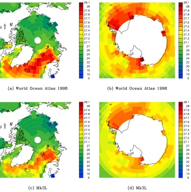
Figure 3.1 shows the annual-maximum surfaceσθ, according to the World Ocean
Atlas 1998 and the Mk3L ocean model spin-up run O-DEF (Section 2.3.2). The peak values encountered in the key regions of deep water formation are also shown in Table 3.1; the excessively buoyant nature of the surface waters in the model is apparent.
In the Southern Ocean, the peak surface densities for both the World Ocean Atlas 1998 and the Mk3L ocean model, of 28.06 kgm−3
and 27.76 kgm−3
respectively, occur in the southwestern Ross Sea. The next highest surface densities occur in the Weddell Sea, with a simulated peak surface density of 27.73 kgm−3
3.3. THE DEFAULT MODEL RESPONSE 63
Figure 3.1: The annual-maximum surface σθ (kgm−3): (a), (b) the World Ocean
World Ocean Mk3L Model Atlas 1998 ocean discrepancy
[image:8.595.133.412.108.180.2]Ross Sea 28.06 27.76 -0.30 Weddell Sea 27.98 27.73 -0.25 Nordic Seas 27.96 27.72 -0.24
Table 3.1: The peak surface σθ (kgm−3) in regions of deep water formation: the
World Ocean Atlas 1998, the Mk3L ocean model (average for the final 100 years of run O-DEF), and the model discrepancy. The World Ocean Atlas 1998 data has been area-averaged onto the Mk3L ocean model grid.
Weddell Sea. The peak surface density in this region, according to the World Ocean Atlas 1998, is 27.96 kgm−3
, although a slightly higher density of 27.98 kgm−3 occurs in the southeastern Weddell Sea. A peak surface density of 27.98 kgm−3
also occurs in Prydz Bay, at 73◦
E, 69◦
S; the simulated surface density at this point is just 27.53 kgm−3
.
In the Arctic, the World Ocean Atlas 1998 features a peak surface density of 27.96 kgm−3
, which occurs in the Nordic (Greenland-Iceland-Norwegian) Seas. The peak surface density simulated by the model in this region is just 27.72 kgm−3
. (The maximum simulated surface density in the Arctic is 27.80 kgm−3
, but this occurs in the Barents Sea, at 45◦
E, 75◦
N, and is therefore located outside the regions of deep water formation.)
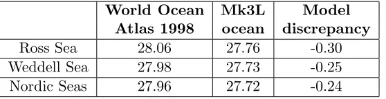
In the regions of Antarctic Bottom Water and North Atlantic Deep Water for-mation, the peak densities of the simulated surface waters are therefore too buoyant by ∼0.25–0.3 kgm−3. This offers a potential explanation for the buoyant nature of the simulated deep ocean (Section 2.5.1), and shall therefore now be studied further. The simulated and observed annual cycles in sea surface temperature, salinity and density in the three regions of deep water formation are shown in Figures 3.2, 3.3 and 3.4. The discrepancies in the simulated annual-mean surface density are small (being -0.01, -0.04 and -0.12 kgm−3
for the Ross, Weddell and Nordic Seas respectively), with the failure to simulate the peak surface densities arising from the failure by the model to correctly simulate the magnitude of the annual cycle.
Figures 3.2, 3.3 and 3.4 reveal three distinct errors in the simulated sea surface temperature and salinity:
• an error in the annual mean
• an error in the amplitude of the annual cycle
• a phase lag between the simulated and observed fields
3.3. THE DEFAULT MODEL RESPONSE 65
Figure 3.2: The monthly-mean sea surface temperature, salinity andσθin the
south-western Ross Sea, for the World Ocean Atlas 1998 (red) and the Mk3L ocean model (green, average for the final 100 years of run O-DEF): (a) sea surface tempera-ture, (b) sea surface salinity, and (c) sea surface σθ. The values plotted are for
the gridpoint located at 163◦ E, 75◦
Figure 3.3: The monthly-mean sea surface temperature, salinity andσθ in the
west-ern Weddell Sea, for the World Ocean Atlas 1998 (red) and the Mk3L ocean model (green, average for the final 100 years of run O-DEF): (a) sea surface temperature, (b) sea surface salinity, and (c) sea surfaceσθ. The values plotted are averages for
the two gridpoints located at 56◦ W, 72◦
S, and 56◦ W, 68◦
3.3. THE DEFAULT MODEL RESPONSE 67
Figure 3.4: The monthly-mean sea surface temperature, salinity andσθin the Nordic
(Greenland-Iceland-Norwegian) Seas, for the World Ocean Atlas 1998 (red) and the Mk3L ocean model (green, average for the final 100 years of run O-DEF): (a) sea surface temperature, (b) sea surface salinity, and (c) sea surface σθ. The values
plotted are averages for the 12 gridpoints which cover the region 14◦ W–8◦
E, 67◦ – 76◦
These errors must be rectified if realistic high-latitude sea surface temperature and salinity fields, and hence realistic high-latitude surface densities, are to be ob-tained within the model.
3.3.1 Errors in the annual-mean climate
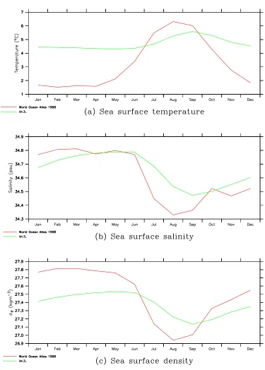
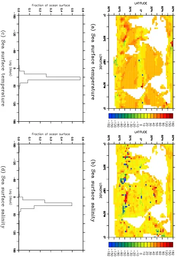
Figure 3.5 shows the annual-mean errors in the simulated SST and SSS, relative to the World Ocean Atlas 1998 values which were imposed as the surface boundary condition; the errors are as large in magnitude as 3.86◦
C and 0.752 psu respectively. A consequence of the relaxation boundary condition (Equations 3.1 and 3.2) is that theremust be errors in the annual-mean SST and SSS, wherever advection and diffusion give rise to non-zero annual-mean surface fluxes. Comparing Figure 3.5 with Figures 2.21b and 2.22b, the linear relationship between the annual-mean SST (or SSS) error, and the annual-mean surface heat flux (or surface salinity tendency), is apparent. The maximum annual-mean SST error of 3.86◦
C corresponds to an annual-mean surface heat flux of 229 Wm−2
(utilising Equation 3.1), while the max-imum annual-mean SSS error of 0.752 psu corresponds to an annual-mean surface salinity tendency of 13.7 psu/year (via Equation 3.2).
3.3.2 Errors in the amplitude of the annual cycle
Figure 3.6 shows the amplitude of the annual cycle in the simulated SST and SSS, expressed as a fraction of the amplitude in the annual cycle of the World Ocean Atlas 1998 SST and SSS. If Tn andT are the monthly-mean and annual-mean SST
(or SSS) respectively, then the root-mean-square amplitude of the annual cycle is given by a= " 1 12 12 X n=1
(Tn−T)2
#1/2
(3.6)
Letaobsbe the root-mean-square amplitude of the observed annual cycle,
accord-ing to the World Ocean Atlas 1998, and letamodbe the root-mean-square amplitude
of the simulated annual cycle, according to the Mk3L ocean model. The response of the model can be studied by expressing the simulated amplitude as a fraction of the observed amplitude, as follows:
r = amod
aobs
(3.7)
3.3. THE DEFAULT MODEL RESPONSE 69
Figure 3.5: The annual-mean sea surface temperature and salinity for the Mk3L ocean model (average for the final 100 years of run O-DEF), expressed as anomalies relative to the World Ocean Atlas 1998: (a) sea surface temperature (◦
3.4. MODIFYING THE RELAXATION BOUNDARY CONDITION 71
3.3.3 Phase lags between the simulated and observed climate
Figure 3.7 shows the lag of maximum correlation between the Mk3L ocean model SST and SSS, and the World Ocean Atlas 1998 data. This lag is calculated from the monthly-mean values as follows:
1. Linear interpolation in time is used to estimate daily values, for both the Mk3L ocean model and the World Ocean Atlas 1998.
2. For each integer value ofn from -182 to +182:
(a) the ocean model values are shifted forward in time by ndays
(b) the correlation coefficient is calculated between the phase-shifted ocean model values, and the World Ocean Atlas 1998 values
3. The value of nwhich maximises the correlation coefficient is called the lag of maximum correlation.
The area-weighted global-mean lags are 31.7 and 22.1 days in the case of the SST and SSS respectively, with unimodal distributions which are tightly clustered around the means. At some gridpoints, particularly in the case of the SSS, the above technique does not produce a meaningful value for the lag; this can occur when either the simulated or observed values do not exhibit a distinct annual cycle.
3.4
Modifying the relaxation boundary condition
Equations 3.1 and 3.2 indicate two ways in which the relaxation boundary condition can be modified:
1. the relaxation constant γ can be varied
2. the prescribed sea surface temperature Tobs and sea surface salinity Sobs can
be modified
Each of these modifications shall now be considered in turn.
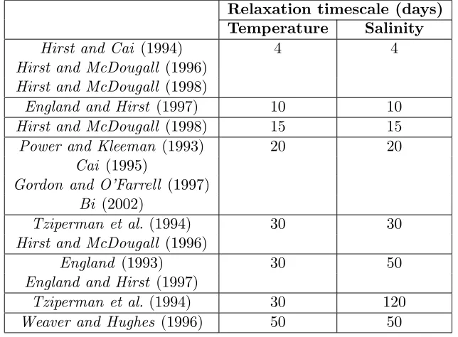
3.4.1 The relaxation timescale
The relaxation timescales used in some of the modelling studies referred to herein are shown in Table 3.2, and are typically of order one month. Hirst and Cai (1994) and subsequent studies, however, choose to use a much shorter timescale of 4 days, as they find that it improves the realism of the water mass properties within their model.
3.4. MODIFYING THE RELAXATION BOUNDARY CONDITION 73
Relaxation timescale (days) Temperature Salinity
Hirst and Cai (1994) 4 4
Hirst and McDougall (1996)
Hirst and McDougall (1998)
England and Hirst (1997) 10 10
Hirst and McDougall (1998) 15 15
Power and Kleeman (1993) 20 20
Cai (1995)
Gordon and O’Farrell (1997)
Bi (2002)
Tziperman et al. (1994) 30 30
Hirst and McDougall (1996)
England (1993) 30 50
England and Hirst (1997)
Tziperman et al. (1994) 30 120
[image:17.595.165.487.109.346.2]Weaver and Hughes (1996) 50 50
Table 3.2: The relaxation timescales used in some of the studies referred to herein.
Timescales such as that employed by Hirst and Cai (1994), however, improve the simulated SST and SSS at the expense of poorer simulated surface fluxes and internal transport (Pierce, 1996), with the surface fluxes exhibiting unrealistically large spatial and temporal variability (e.g. Hirst and McDougall, 1996; Bi, 2002). This tends to increase the mismatch with the atmosphere model surface fluxes, and leads to an undesirable increase in the magnitude of the flux adjustments diagnosed for use within the coupled model.
The use of very short relaxation timescales also degrades other aspects of the simulated ocean climate. Pierce(1996) notes that the stability characteristics of the thermohaline circulation are distorted, while Killworth et al. (2000) note that the western boundary currents are severely degraded, and that features such as eddies and planetary waves are suppressed.
3.4.2 Surface tracers
A number of studies have modified the prescribed surface tracers in order to im-prove the realism of the model climate. A common technique has been to modify the prescribed SST and SSS at high latitudes; there are two motivations for these modifications:
• in the absence of a sea ice model, to allow for the effects of brine rejection (e.g. Toggweiler and Samuels, 1995; Weaver and Hughes, 1996)
• to correct for perceived deficiencies in the observed SST and SSS, particularly with regard to a “fair weather” bias at high latitudes (e.g. England, 1993;
In some of these studies, the modifications are used in conjunction with the application of perpetual winter surface tracers in both hemispheres (e.g. Hirst and Cai, 1994; Hirst and McDougall, 1996, 1998).
“Fair weather” biases in observational climatologies are noted by Weaver and Hughes (1996) and Duffy and Caldeira (1997). These biases arise from a lack of observations beneath sea ice in both the Arctic and Antarctic, and from a tendency for observations of sea surface temperature and salinity to be made only under fair weather conditions. The observed SSTs therefore tend to be too warm, and the observed SSSs too fresh. To compensate for these biases, Weaver and Hughes
(1996) modify the observational climatology of Levitus (1982) at high latitudes. Over the Arctic Ocean, they replace the observed SSTs and SSSs with the average temperatures and salinities, respectively, of the upper 50 m of the water column. In the Ross and Weddell Seas, the observed SSTs are replaced with values of -1.85◦
C, and the observed SSSs are replaced with values of 35.1 psu.
Weaver and Hughes (1996) find that these modifications lead to the diagnosis of very large flux adjustments in the Southern Ocean. Bi (2002), however, does not encounter this problem. One possible explanation for this discrepancy is that the model employed by Bi (2002) incorporates Gent-McWilliams eddy diffusion (Gent and McWilliams, 1990), while that employed by Weaver and Hughes (1996) does not. Models which do not incorporate Gent-McWilliams eddy diffusion are prone to excessive convection in the high-latitude Southern Ocean, and can experience very unrealistic surface fluxes as a result (e.g. Hirst et al., 2000).
Bi (2002) experiments with a more systematic approach towards modifying the surface tracers, also with the aim of improving the peak densities of the surface waters in the regions of deep water formation. He employs an iterative approach, as follows:
1. The ocean model is spun up using relaxation boundary conditions, with ob-served values for the SST and SSS being prescribed.
2. The anomaly in the simulated SST, ∆T =Tmod−Tobs, is diagnosed at each
gridpoint and for each month of the year.
3. These anomalies are subtracted from the observed SST, obtaining a timeseries of modified SSTs.
4. The ocean model spin-up run is continued, with the modified SSTs being prescribed.
5. SST anomalies are diagnosed from the new run, and are used to further modify the prescribed SSTs.
This process is repeated several times. However, numerical problems force him to confine the modifications to latitudes north of 40◦
N and south of 60◦
S, and to abandon attempts to apply the same technique to the SSS. His approach therefore has a relatively restricted application.
3.5. VARYING THE RELAXATION TIMESCALE 75
to the prescribed surface tracers. However, this method is dependent upon an obser-vational climatology for the surface heat flux, and therefore introduces a potentially significant source of error. An alternative would be to employ this approach to derive apparent surface tracers such that, when the simulated SST is equal to the prescribed value, the surface heat flux would be equal to the value derived from an atmosphere model spin-up run. This would avoid the need to apply adjustments to the heat flux within the coupled model. However, this approach would also intro-duce a potential source of error, as the surface fluxes calculated by the atmosphere model will reflect any errors in the model physics, and in the boundary conditions on the stand-alone atmosphere model.
A further alternative is the approach of Pierce (1996). Using Fourier analysis, he estimates the errors in the simulated SST that will arise when an ocean model is spun up using the relaxation boundary condition. He then uses these errors to calculate a timeseries of apparent surface air temperatures. This method avoids the dependence of the method of Haney (1971) and Han (1984) upon an observational climatology for the surface heat flux. While it is successful at reducing the differences between the observed and simulated SST, it is hampered by the assumption that there is no internal transport of heat within the ocean.
3.5
Varying the relaxation timescale
Having considered the ways in which the relaxation boundary condition might be modified, the remainder of this chapter studies the dependence of the simulated ocean climate upon the relaxation timescale. In this section, a simple theoretical model is used to investigate this relationship; in Section 3.6, the response of the Mk3L ocean model is studied.
The dependence of the simulated ocean climate upon the prescribed sea surface temperatures and salinities is studied in Chapter 4.
3.5.1 The response of a slab ocean model
Consider a slab ocean model, being one in which the evolution of the temperature and salinity at each gridpoint is determined solely by the relevant surface flux. Let the prescribed sea surface temperature be Tobs(t), wheretrepresents time in days,
and let the response of the model beTmod(t). Ifτ represents the relaxation timescale
in days, then the evolution of Tmod is determined by the equation
dTmod
dt =
1
τ(Tobs−Tmod) (3.8)
Let the model be forced with a sine wave of amplitudesobs, and frequencyω:
Tobs =aobssinωt (3.9)
Let the equilibrium response of the model also be a sine wave, which exhibits both a phase lag φand an amplificationr relative to the forcing:
Substituting Equations 3.9 and 3.10 into Equation 3.8:
raobsωcos(ωt−φ) = 1
τ [aobssinωt−raobssin(ωt−φ)] (3.11)
Substitutingωt= 0 into Equation 3.11, and dividing through by raobscosφ:
ω= 1
τ tanφ (3.12)
A solution is therefore obtained for φ:
φ= tan−1
ωτ (3.13)
Substitutingωt=φ into Equation 3.11, and dividing through byaobsω, a
solu-tion is also obtained forr:
r= 1
ωτ sinφ (3.14)
Let the relaxation timescale be τ = 20 days, being the default timescale em-ployed by the Mk3L ocean model, and let the period of the sine wave be 365 days, corresponding to the annual cycle. Thusω= 2π/(365 days), and Equations 3.13 and 3.14 give φ≈ 19.0◦ and r ≈0.946 respectively. The response of this simple model is therefore only slightly attenuated relative to the forcing signal, and it experiences a time lag of just 19.3 days (i.e. 19.0◦
/360◦
×365 days).
The observed annual cycle in the sea surface temperature or salinity will not, in general, be a perfect sine wave. The observed timeseries at any point on the Earth’s surface can, however, be expressed as a truncated Fourier series, thus:
Tobs(t) =a0+
N
X
n=1
ansin(nωt+φn) (3.15)
The truncation arises from the finite temporal resolution of any observational timeseries. For a dataset such as the World Ocean Atlas 1998, which contains monthly-mean data, the sampling interval is one month. The Nyquist frequency (e.g. Wilks, 1995) is therefore equal to 0.5 months−1
= 6 years−1
, and the upper boundN in Equation 3.15 will be equal to 6.
Equation 3.8 is a linear differential equation, and can therefore be solved sepa-rately for each component of the Fourier series. The solutions are found to be
φn = tan−
1
nωτ (3.16)
rn =
1
nωτ sinφn (3.17)
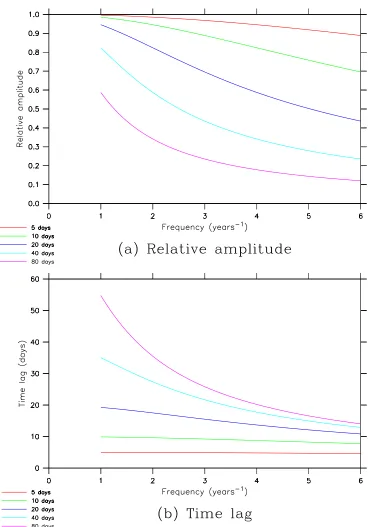
These solutions are plotted in Figure 3.8, for values of nfrom 1 to 6, and for re-laxation timescales varying from 5 to 80 days. It can be seen that, as the frequency of the applied signal increases, the response of the model becomes increasingly at-tenuated, although the time lag also decreases. For a relaxation timescale of 20 days,
3.5. VARYING THE RELAXATION TIMESCALE 77
A reduction in the relaxation timescale can be seen to improve the response of the model, increasing the amplitude and reducing the time lag.
The World Ocean Atlas 1998 sea surface temperatures and salinities can be analysed within this context. Figure 3.8 shows that the amplitude of the simulated annual cycle is greatest for a sine wave of period one year, but that the same is also true for the phase lag. Hence, as the annual cycle in the observed SST or SSS becomes increasingly dominated by higher-frequency harmonics, the amplitude of the simulated annual cycle will decrease, but so will the phase lag. To investigate this further, a quantity is defined which shall be referred to herein as the sinusoidality. This represents the fraction of the total variance which is associated with a period of one year and, in terms of the coefficients defined in Equation 3.15, is given by
s = a
2 1 N X n=1 a2 n (3.18)
If the annual cycle in the observed sea surface temperature or salinity is a perfect sine wave, then the sinusoidality will be equal to 1. However, as increasing variance becomes associated with higher-frequency harmonics, the sinusoidality will decrease. Figure 3.9 shows the sinusoidality for the World Ocean Atlas 1998 sea sur-face temperature and salinity, after interpolation onto the Mk3L ocean model grid. Throughout the sub-tropics and mid-latitudes, the SST has a sinusoidality which ex-ceeds 0.9, indicating that at least 90% of the variance is associated with a sine wave of period one year; only in the tropics and at high latitudes do the higher-frequency harmonics begin to dominate. The area-weighted global-mean sinusoidality is equal to 0.85.
The sea surface salinity, however, exhibits a distinct annual cycle in only very limited regions, mostly in the Northern Hemisphere. The sinusoidality exceeds 0.9 over just 4% of the surface of the ocean, in sharp contrast to the figure of 61% in the case of the SST. The area-weighted global-mean sinusoidality is just 0.47, indicating that the SSS generally exhibits a very indistinct annual cycle.
The equilibrium response of the slab ocean model, when forced with the same World Ocean Atlas 1998 sea surface temperatures and salinities that were used to spin up the Mk3L ocean model, is now investigated. Figure 3.10 shows the values for the relative amplitude and the time lag. The generally sinusoidal nature of the annual cycle in the SST in the sub-tropics, and at mid-latitudes, is reflected in values for the relative amplitude and the time lag which approach the theoretical maximum values, derived above, of 0.946 and 19.3 days respectively. In contrast, the less sinusoidal nature of the annual cycle in the SSS is reflected in much smaller relative amplitudes, and in shorter time lags.
3.5. VARYING THE RELAXATION TIMESCALE 79
3.5. VARYING THE RELAXATION TIMESCALE 81
relative amplitudes and time lags that are highly spatially variable, and the lags are generally shorter than for the sea surface temperature.
All these features are consistent with the behaviour of the slab ocean model. Indeed, the only large-scale features of the Mk3L ocean model that are not con-sistent with the slab ocean model are the strong sea surface temperature response in the tropics, and the fact that the relative amplitudes can exceed 1. Both these discrepancies can be attributed to either lateral or vertical fluxes within the ocean, which the slab ocean model cannot represent.
Surface fluxes
The slab ocean model can also be used to investigate the effect of a change in the relaxation timescale on the magnitude of the surface fluxes. If cv is the volumetric
heat capacity of seawater and ∆z the thickness of the slab ocean, then the surface heat flux F is given by
F = d
dt(cv∆z Tmod) (3.19)
Let the model be forced by a prescribed sea surface temperature of amplitude
aobs and frequencynω, and let the equilibrium response of the model be
Tmod=rnaobssin(nωt−φn) (3.20)
Substituting Equation 3.20 into Equation 3.19:
F = d
dt[cv∆z rnaobs sin(nωt−φn)] (3.21)
= cv∆z rnaobsn ω cos(nωt−φn) (3.22)
Expressing the surface heat flux as
F =F0cos(nωt−φn) (3.23)
the ratio between the amplitude of the surface heat flux, and the amplitude of the prescribed SST, is therefore given by
F0
aobs
=cv∆z rnn ω (3.24)
Let cv = 4.1×10⁶ Jm−3K−1 and ∆z = 25 m, being the values used within the Mk3L ocean model. Using the values of rn given by Equation 3.17, the resulting
solutions are plotted in Figure 3.11.
For a sine wave of period one year, the amplitude of the surface heat flux is only weakly dependent upon the relaxation timescale, increasing from 12.0 Wm−2
K−1 to 20.3 Wm−2
K−1
as the relaxation timescale is reduced from 80 to 5 days. rn tends
Figure 3.11: The amplitude of the surface heat flux, per unit amplitude of the applied sea surface temperature, for the equilibrium response of a slab ocean model to sinusoidal forcing. The relaxation boundary condition is employed, using relaxation timescales of 5 days (red), 10 days (green), 20 days (dark blue), 40 days (light blue) and 80 days (purple).
lim
τ→0
F
0
Aobs
=cv∆z n ω (3.25)
The limiting flux is equal to 20.4 Wm−2 K−1
for a sine wave of period one year, and 123 Wm−2
K−1
for a sine wave of period two months.
Figure 3.11 suggests that, when an ocean model is forced with observed sea sur-face temperatures and salinities, the sursur-face freshwater fluxes will be more sensitive to a reduction in the relaxation timescale than the surface heat fluxes. The annual cycle in the observed SST is generally dominated by a sine wave of period one year, in which case the amplitude of the surface heat flux is only weakly dependent upon the relaxation timescale. The annual cycle in the observed SSS is generally domi-nated by higher-frequency harmonics, however, in which case the dependence upon the relaxation timescale is stronger in the case of the surface freshwater flux.
3.5.2 The response of a mixed-layer ocean
3.5. VARYING THE RELAXATION TIMESCALE 83
the evolution of the SST and SSS within an ocean general circulation model. In particular, the existence of a homogeneous mixed layer would tend to attenuate the response of the model to external forcing.
However, the theoretical model can readily be extended to make a crude al-lowance for the presence of a mixed layer within the ocean. If a homogeneous mixed layer exists within the ocean, then it can be assumed that any flux of heat (or freshwater) into the ocean will be instantaneously and uniformly distributed, in the vertical direction, throughout the mixed layer. If the thickness of the mixed layer is α∆z, where ∆zis the thickness of the upper layer of the model and α is greater than or equal to 1, then Equation 3.8 becomes
dTmod
dt =
1
ατ(Tobs−Tmod) (3.26)
The only difference between Equations 3.8 and 3.26 is that the relaxation time-scale τ has been replaced with ατ. The solutions to Equation 3.26 are therefore given by the solutions to Equation 3.8, with the relaxation timescale replaced with an effective relaxation timescale τ∗
=ατ. The surface heat flux is also larger by a factor α, reflecting the increased heat capacity of the mixed-layer ocean relative to that of the upper layer of the model. The solutions to Equation 3.26 are therefore:
φ = tan−1
αωτ (3.27)
r = 1
αωτ sinφ (3.28)
F0
aobs
= cv∆z r α ω (3.29)
The solutions for forcing by a sine wave of period one year are plotted in Fig-ure 3.12, for values ofα from 1 to 100, and for relaxation timescales ranging from 5 to 80 days. As the depth of the mixed-layer ocean is increased, the amplitude of the model response decreases, while the time lag and surface heat flux increase. The limiting solutions as α tends towards infinity are as follows:
lim
α→∞φ = 90 ◦
(= 91.25 days) (3.30)
lim
α→∞r = 0 (3.31)
lim α→∞ F 0 aobs
= cv∆z
τ (3.32)
3.5.3 Summary
These investigations into the response of a simple theoretical model provide insight into the response that might be expected from an ocean general circulation model:
3.6. THE RESPONSE OF THE MK3L OCEAN MODEL 85
Run Relaxation Duration (years) timescale Asynchronous Synchronous
(days) timestepping timestepping
O-5d 5 4000 500
O-7.5d 7.5 3000 500
O-10d 10 3000 500
O-15d 15 4000 500
O-DEF 20 4000 500
O-30d 30 5000 500
O-40d 40 5000 500
O-60d 60 5000 500
[image:29.595.185.469.107.277.2]O-80d 80 6000 500
Table 3.3: A summary of the Mk3L ocean model spin-up runs in which the relaxation timescale was varied.
• Increasing the frequency of the forcing signal reduces the amplitude of the model response, reduces the time lag, and increases the magnitude of the surface fluxes.
• An increase in the depth of the mixed layerreduces the amplitude of the model response, increases the time lag, and increases the magnitude of the surface fluxes.
3.6
The response of the Mk3L ocean model
A series of spin-up runs was conducted using the Mk3L ocean model. These runs are summarised in Table 3.3; they are identical to run O-DEF (Section 2.3.2), with the exception that the relaxation timescale was varied from 5 to 80 days. Each run was integrated under asynchronous timestepping until the convergence criteria were sat-isfied (i.e. that the rates of change in global-mean potential temperature and salinity, on each model level, were less than 0.005◦
C/century and 0.001 psu/century respec-tively). A further 500 years of integration was then conducted under synchronous timestepping, by which time the convergence criteria were once again satisfied.
The dependence of the simulated ocean climate upon the relaxation timescale is assessed in the following sections.
3.6.1 Annual-mean errors
The root-mean-square (RMS) errors in the annual-mean sea surface temperature and salinity, relative to the World Ocean Atlas 1998, are plotted in Figure 3.13 as a function of the relaxation timescale. Let the error in the sea surface temperature (or salinity) be defined as ∆T =Tmod−Tobs, whereTmodandTobsare the simulated
and observed sea surface temperature (or salinity) respectively. If the error at each gridpoint is ∆Ti,j, and the area of the gridbox centred on that gridpoint is Ai,j,
∆Trms= X i X j
A2i,j∆Ti,j2
1/2
X
i
X
j
Ai,j (3.33)
The errors can be seen to be very sensitive to the relaxation timescale. The RMS error in the annual-mean SST increases from 0.17◦
C to 1.53◦
C as the relaxation timescale is increased from 5 to 80 days, while that in the annual-mean SSS increases from 0.024 psu to 0.224 psu.
3.6.2 Relative amplitudes and time lags
The global-mean relative amplitude and time lag, for both the sea surface tempera-ture and salinity, are plotted in Figure 3.14 as a function of the relaxation timescale. The area-weighted global means are shown; if the relative amplitude (or time lag) at each gridpoint is ri,j, and if the area of the gridbox centred on that gridpoint is Ai,j, then the area-weighted global-mean relative amplitude (or time lag)r is given
by r= X i X j
Ai,jri,j
X i X j Ai,j (3.34)
Consistent with the response of the simple theoretical model (Sections 3.5.1 and 3.5.2), the amplitude of the model response decreases as the relaxation timescale is increased, while the time lag decreases. In the case of the SST, the global-mean relative amplitude decreases from 0.836 to 0.239 as the relaxation timescale is increased from 5 to 80 days, while the global-mean time lag increases from 10.7 to 49.1 days. Similar behaviour is exhibited in the case of the SSS, with a decrease in the global-mean relative amplitude from 0.746 to 0.258, and an increase in the global-mean time lag from 6.4 to 37.3 days.
3.6. THE RESPONSE OF THE MK3L OCEAN MODEL 87
3.6. THE RESPONSE OF THE MK3L OCEAN MODEL 89
3.6.3 Densities of high-latitude surface waters
Figure 3.15 shows the peak surface water density, as a function of the relaxation timescale, for each of the three deep water formation regions which were studied in Section 3.3. The peak densities at each gridpoint, for runs O-5d, O-10d, O-40d and O-80d, are also shown in Figures 3.16 and 3.17, for the Antarctic and Arctic respectively. (Values for run O-DEF are shown in Figure 3.1.)
The peak densities are highly sensitive to the relaxation timescale. However, even when the timescale is reduced to 5 days, the surface waters remain too buoyant. The peak surface densities in this case are 27.90, 27.81 and 27.88 kgm−3
, for the southwestern Ross Sea, western Weddell Sea and Nordic Seas respectively. These densities represent light biases, relative to the World Ocean Atlas 1998, of 0.16, 0.15 and 0.08 kgm−3
respectively. While these figures represent a considerable improvement on the biases of∼0.25–0.3 kgm−3enountered in the case of run O-DEF (Section 3.3), the peak high-latitude surface water densities remain inadequate.
3.6.4 Water properties
Vertical profiles of potential temperature, salinity and potential density are shown in Figure 3.18, for the World Ocean Atlas 1998 and for Mk3L ocean model runs O-5d, O-10d, O-DEF, O-40d and O-80d. As a result of the increased peak densities of the high-latitude surface waters, the density of the deep ocean increases as the relaxation timescale is reduced. This is achieved through an increase in the salinity of the deep ocean, with the relaxation timescale having little impact upon the temperature profile.
These trends are confirmed by Figure 3.19, which shows the mean potential temperature, salinity and potential density for the deep ocean (2350–4600 m, as defined in Chapter 2), as a function of the relaxation timescale. While the most realistic deep ocean salinity and density are achieved when the relaxation timescale is reduced to 5 days, it remains too fresh by 0.13 psu, and too buoyant by 0.04 kgm−3
. The deep ocean temperature is only weakly dependent upon the relaxation timescale, being consistently too cold by ∼1◦C.
3.6.5 Circulation
The rates of North Atlantic Deep Water (NADW) and Antarctic Bottom Water (AABW) formation are plotted in Figure 3.20 as a function of the relaxation time-scale.
The rate of NADW formation declines as the relaxation timescale is increased, decreasing from 16.1 to 10.5 Sv as the timescale is increased from 5 to 80 days. This behaviour can be attributed to the strong dependence of the peak surface water density in the Nordic Seas upon the relaxation timescale (Figure 3.15); the peak density decreases by 0.49 kgm−3
, from 27.88 to 27.39 kgm−3
, as the timescale is increased from 5 to 80 days. In contrast, the density of the deep ocean decreases by just 0.29 kgm−3
, from 27.76 to 27.47 kgm−3
Figure 3.15: The annual-maximum surface σθ (kgm−3) for the World Ocean Atlas
3.6. THE RESPONSE OF THE MK3L OCEAN MODEL 91
Figure 3.16: The annual-maximum surface σθ (kgm−3) for the Mk3L ocean model
Figure 3.17: The annual-maximum surface σθ (kgm−3) for the Mk3L ocean model
3.6. THE RESPONSE OF THE MK3L OCEAN MODEL 93
Figure 3.18: The global-mean potential temperature, salinity andσθ on each model
level for the World Ocean Atlas 1998 (black), and for Mk3L ocean model runs O-5d (red), O-10d (green), O-DEF (dark blue), O-40d (light blue) and O-80d (purple): (a) potential temperature, (b) salinity, and (c) σθ. The World Ocean Atlas 1998
Figure 3.19: The mean potential temperature, salinity and σθ for the deep ocean
(2350–4600 m), for the World Ocean Atlas 1998 (black), and for the Mk3L ocean model (red, averages for the final 100 years of runs O-5d, O-7.5d, O-10d, O-15d, O-DEF, O-30d, O-40d, O-60d and O-80d): (a) potential temperature, (b) salinity, and (c) σθ. The World Ocean Atlas 1998 data has been volume-averaged onto the
3.6. THE RESPONSE OF THE MK3L OCEAN MODEL 95
Figure 3.20: The rates of North Atlantic Deep Water formation (red) and Antarctic Bottom Water formation (green) for the Mk3L ocean model (averages for the final 100 years of runs O-5d, O-7.5d, O-10d, O-15d, O-DEF, O-30d, O-40d, O-60d and O-80d).
The rate of AABW formation increases, however, from 7.8 to 12.3 Sv; this can also be attributed to changes in the stratification of the water column. The peak surface water densities in the Ross and Weddell Seas decrease by 0.28 and 0.23 kgm−3
, respectively, as the timescale is increased from 5 to 80 days. These decreases are smaller than the reduction of 0.29 kgm−3
in the density of the deep ocean, and the water column in the Southern Ocean therefore becomes decreasingly stratified. As a result, the rate of AABW formation increases.
3.6.6 Annual-mean surface fluxes
3.6. THE RESPONSE OF THE MK3L OCEAN MODEL 97
The annual-mean surface fluxes exhibit only a limited dependence upon the re-laxation timescale. While this might seem surprising, it should be borne in mind that non-zero annual-mean surface fluxes only arise as a result of the ocean circula-tion, and as a result of diffusive processes within the ocean. Without these processes, there would be no net fluxes of heat or salt through either the lateral walls or the bases of the surface gridboxes, and the annual-mean surface fluxes would be equal to zero. In the previous section, the ocean circulation was shown to exhibit only a lim-ited dependence upon the relaxation timescale; the dependence of the annual-mean surface fluxes upon the relaxation timescale is therefore similarly limited.
The annual-mean flux adjustments are even more weakly dependent upon the relaxation timescale. This arises because the flux adjustments depend upon the surface fluxes simulated by both the ocean model and the atmosphere model. As the relaxation timescale is increased, the magnitude of the ocean model fluxes de-creases, and the atmosphere model surface fluxes become increasingly dominant in determining the magnitude of the flux adjustments. The flux adjustments therefore become increasingly independent of the relaxation timescale.
The annual-mean surface heat flux and salinity tendency adjustments, diagnosed from runs O-5d, O-10d, O-40d and O-80d, are shown in Figures 3.22 and 3.23 re-spectively; those diagnosed from run O-DEF are shown in Figures 2.21 and 2.22. While the magnitude of the annual-mean flux adjustments exhibits a weak depen-dence upon the relaxation timescale, the spatial structure remains unchanged. This indicates that the need for flux adjustments arises from inconsistencies between the oceanic transports of heat and salt, as simulated by the ocean model and as implied by the atmosphere model. The flux adjustments therefore represent deficiencies in the model physics, rather than arising as a result of stochastic variability in the simulated surface fluxes.
3.6.7 Amplitudes of surface fluxes
The area-weighted global-mean amplitudes of the annual cycles in the simulated surface fluxes are plotted in Figure 3.24, along with the area-weighted global-mean amplitudes of the annual cycles in the flux adjustments diagnosed for the coupled model. If Fn and F are the monthly-mean and annual-mean surface flux (or flux
adjustment) respectively, then the amplitude of the annual cycle is given by Equa-tion 3.6, i.e.
a= " 1 12 12 X n=1
(Fn−F)2
#1/2
(3.35)
If the amplitude of the annual cycle at each gridpoint is ai,j, and the area of
the gridbox centred on that gridpoint is Ai,j, then the area-weighted global-mean
amplitude is given by Equation 3.34, i.e.
Figure 3.22: The annual-mean surface heat flux adjustment (Wm−2
3.6. THE RESPONSE OF THE MK3L OCEAN MODEL 99
3.6. THE RESPONSE OF THE MK3L OCEAN MODEL 101
Consistent with the response of the simple theoretical model (Sections 3.5.1 and 3.5.2), the amplitudes of the surface fluxes decrease as the relaxation timescale is increased. The global-mean amplitude of the surface heat flux decreases from 82.6 to 18.7 Wm−2
as the relaxation timescale is increased from 5 to 80 days. Similarly, the global-mean amplitude of the surface salinity tendency decreases from 3.13 to 0.58 psu/year.
It should be noted that, as the relaxation timescale is increased, the global-mean amplitudes decrease by factors of 4.42 and 5.42, in the case of the surface heat flux and surface salinity tendency respectively. This confirms the prediction made in Section 3.5.1, that the less sinusoidal nature of the annual cycle in the observed sea surface salinity would make the surface salinity tendency more sensitive to changes in the relaxation timescale.
The global-mean amplitude of the surface heat flux adjustment reaches a mini-mum of 47.5 Wm−2
at a relaxation timescale of 7.5 days. As the timescale is either increased or decreased, the surface heat fluxes simulated by the stand-alone ocean model become increasingly incompatible with those simulated by the stand-alone atmosphere model, and the amplitude of the heat flux adjustments increases. In contrast, the lack of spatial correlation between the surface salinity tendencies sim-ulated by the stand-alone atmosphere and ocean models (Figure 2.22) is such that there is no optimal relaxation timescale. As the timescale is increased, the magni-tude of the surface salinity tendencies simulated by the ocean model decreases, and the magnitude of the surface salinity tendency adjustments therefore also decreases.
3.6.8 Summary
Reducing the relaxation timescale from its default value of 20 days leads to some improvements in the ocean climate. Consistent with the response of a slab ocean model, the simulated sea surface temperatures and salinities exhibit a more realistic annual cycle, and the phase lags relative to observations are reduced. The resulting improvement in the properties of the high-latitude surface waters leads to increases in the salinity and density of the deep ocean, and enhanced North Atlantic Deep Water formation.