environment: construction and analysis of a stochastic integral projection model
.
White Rose Research Online URL for this paper:
http://eprints.whiterose.ac.uk/1396/
Article:
Childs, D.Z., Rees, M., Rose, K.E. et al. (2 more authors) (2004) Evolution of
size-dependent flowering in a variable environment: construction and analysis of a
stochastic integral projection model. Proceedings of the Royal Society B: Biological
Sciences, 271 (1537). pp. 425-434. ISSN 1471-2954
https://doi.org/10.1098/rspb.2003.2597
[email protected] https://eprints.whiterose.ac.uk/ Reuse
Unless indicated otherwise, fulltext items are protected by copyright with all rights reserved. The copyright exception in section 29 of the Copyright, Designs and Patents Act 1988 allows the making of a single copy solely for the purpose of non-commercial research or private study within the limits of fair dealing. The publisher or other rights-holder may allow further reproduction and re-use of this version - refer to the White Rose Research Online record for this item. Where records identify the publisher as the copyright holder, users can verify any specific terms of use on the publisher’s website.
Takedown
If you consider content in White Rose Research Online to be in breach of UK law, please notify us by
Received22 July 2003
Accepted30 September 2003
Published online14 January 2004
Evolution of size-dependent flowering in a variable
environment: construction and analysis of a
stochastic integral projection model
Dylan Z. Childs
1, Mark Rees
1*, Karen E. Rose
1, Peter J. Grubb
2and Stephen P. Ellner
31Department of Biological Sciences and NERC Centre for Population Biology, Imperial College, Silwood Park,
Ascot SL5 7PY, UK
2Department of Plant Sciences, University of Cambridge, Cambridge CB2 3EA, UK
3Department of Ecology and Evolutionary Biology, Corson Hall, Cornell University, Ithaca, NY 14853-2701, USA
Understanding why individuals delay reproduction is a classic problem in evolutionary biology. In plants, the study of reproductive delays is complicated because growth and survival can be size and age dependent, individuals of the same size can grow by different amounts and there is temporal variation in the environ-ment. We extend the recently developed integral projection approach to include size- and age-dependent demography and temporal variation. The technique is then applied to a long-term individually structured
dataset for Carlina vulgaris, a monocarpic thistle. The parameterized model has excellent descriptive
properties in terms of both the population size and the distributions of sizes within each age class. In
Carlina, the probability of flowering depends on both plant size and age. We use the parameterized model to predict this relationship, using the evolutionarily stable strategy approach. Considering each year separ-ately, we show that both the direction and the magnitude of selection on the flowering strategy vary from year to year. Provided the flowering strategy is constrained, so it cannot be a step function, the model accurately predicts the average size at flowering. Elasticity analysis is used to partition the size- and
age-specific contributions to the stochastic growth rate,s. We usesto construct fitness landscapes and show
how different forms of stochasticity influence its topography. We prove the existence of a unique stochastic
growth rate,s, which is independent of the initial population vector, and show that Tuljapurkar’s
pertur-bation analysis for log(s) can be used to calculate elasticities.
Keywords:fluctuating selection; fitness landscape; stochastic growth rate; evolutionarily stable strategy
1. INTRODUCTION
Natural systems are often highly variable, yet the majority of life-history studies assume a constant density-inde-pendent environment (reviews in Roff 1992 and Stearns 1992). These assumptions allow fitness to be assessed in terms of simple measures of population growth rate such
as r, the intrinsic rate of increase, or R0, the net
repro-ductive rate (Charlesworth 1994). However, this approach is appropriate only in a constant environment, where popu-lation growth is unconstrained or particular forms of den-sity dependence operate (Mylius & Diekmann 1995). When there is environmental stochasticity or a non-equilib-rium attractor, theory predicts that the fitness of a given life-history strategy may be quite different (Tuljapurkar
1990; Rand et al. 1994). For example, in a
density-regu-lated population the fitness of a strategy depends on the other life histories present. Under such conditions, fitness
should be measured using the ‘invasion exponent’, which
is the logarithmic growth rate of an invading population growing in an environment defined by the resident
popu-lation (Metzet al.1992; Mylius & Diekmann 1995).
Fail-ure to use invasibility analysis based on may result in
*Author for correspondence ([email protected]).
Proc. R. Soc. Lond.B (2004)271, 425–434 425 2004 The Royal Society
DOI 10.1098/rspb.2003.2597
imprecise or even qualitatively incorrect predictions about optimal life-history strategies.
Typically, the demography of a structured population is investigated by constructing a matrix model, where indi-viduals are placed into discrete categories defined by age, stage or size class (Caswell 2001). However, such models are not strictly appropriate for continuously structured populations, as the choice of categories may affect the
pre-dictions of the model (Easterlinget al.2000). The
individ-ual-based approach provides an alternative for modelling continuously structured populations. However, though the individual-based approach is flexible, it is compu-tationally inefficient and the underlying models are often difficult to describe. The recently developed integral jection model provides an elegant framework for pro-jecting a continuously structured population in discrete
time (Easterlinget al.2000; Rees & Rose 2002; Childset
al.2003), yet until now this approach was limited to
We use these techniques to explore why organisms defer reproduction, a classic problem in evolutionary biology (Cole 1954). The main benefits of early reproduction accrue through reductions in mortality and generation time, while the costs of early reproduction are reduced fecundity and/or quality of offspring (Cole 1954; Roff 1992; Stearns 1992). In plants, the study of reproductive delays is complicated because plants vary continuously in size and there is enormous variation in growth between individuals. Several studies have attempted to predict the optimal size of flowering in semelparous plants, using a variety of approaches. These approaches include analytical approximations, dynamic state variable models or compu-tationally expensive individual-based models (Kachi &
Hirose 1985; de Jonget al.1989, 2000; Wesselinghet al.
1997; Rees et al. 1999, 2000; Rees & Rose 2002; Rose
et al. 2002). Reeset al. (1999) compared these different approaches by developing a series of parameterized
demo-graphic models of the monocarpic thistleOnopordum
illyr-icumand found that an accurate prediction of flowering
size was possible only when using an individual-based
model. More recently, Roseet al.(2002) were able to
pre-dict the optimal flowering size of another monocarpic
thistle, Carlina vulgaris, using an individual-based
approach. Both these studies emphasized the need to incorporate stochastic variation into life-history analyses.
We explore the evolution of size- and age-dependent
flowering in the monocarpic thistleC. vulgaris. The
prob-ability of flowering inCarlina, as in several other
monocar-pic species, is a function of plant size and age (Klinkhamer
et al.1987; Reeset al.1999; Roseet al. 2002). First, we outline the construction of stochastic integral projection models for monocarpic plants with size- and age-dependent demographic rates. We then summarize the
size- and age-dependent demography of Carlina. Using
invasibility analysis, we then test whether the estimated strategy is adaptive in a stochastic environment. We gener-ate fitness landscapes under different stochasticity regimes to test whether they are consistent with our interpretation of the evolutionarily stable strategy (ESS) calculations. Finally, we carry out elasticity analysis as a further com-parison of mutant fitness in constant and stochastic environments. We prove the existence of a unique
stochas-tic growth rate, s, which is independent of the initial
population vector for the stochastic integral projection model, and show that Tuljapurkar’s perturbation analysis
for log(s) can be used to calculate elasticities
(Tuljapurkar 1990).
2. METHODS
(a) Stochastic integral projection models
The integral projection model can be used to describe how a continuously size-structured population changes in discrete time (Easterlinget al.2000). The state of the population is described by a probability density function,n(x,t), which can intuitively be thought of as the proportion of individuals that are of sizex at timet. The integral projection model for the proportion of indi-viduals that are of size y at time t⫹1, 1 year later, is then given by
Proc. R. Soc. Lond.B (2004)
n(y,t⫹1)=
冕
⍀
[p(x,y)⫹ f(x,y)]n(x,t)dx
=
冕
⍀
k(y,x)n(x,t)dx, (2.1)
wherek(y,x), known as the kernel, describes all possible tran-sitions from sizexto size y, including births. The integration is over the set of all possible sizes,⍀. The kernel is composed of two parts, a fecundity function,f(x,y), and a survival–growth function, p(x,y). To include environmental stochasticity we imagine that a model linking the environment to the demo-graphic rates has been defined. This gives rise to a series of ker-nelsk(0)(x,y),k(1)(x,y), ...,k(t)(x,y) describing the environment at each time-step until yeart. The stochastic integral projection model is then given by
n(y,t⫹1)=
冕
⍀
k(t)(x,y)n(x,t)dx. (2.2)
To extend this basic model to include size- and age-dependent demography we definena(y,t) to be the probability density
func-tion for individuals of sizey and ageain yeart(see Childset al. 2003). The stochastic integral projection model then becomes
n0(y,t⫹1)=
冘
m
a=0
冕
⍀ f(t)a(x,y)na(x,t)dx a=0,
na(y,t⫹1)=
冕
⍀ p(t)
a⫺1(x,y)na⫺1(x,t)dx a⬎0,
(2.3)
wheref(t)
a(x,y) is the fecundity function, p(at)(x,y) is the survival–
growth function of plants of sizexand ageain yeart, andmis maximum plant age. These functions are referred to collectively as the kernel component functions. For a numerical solution, it is convenient to write the model in matrix form as
n(y,t⫹1)=
冕
⍀
K(t)n(x,t)dx, (2.4)
whereK is the matrix
K(t)=
冢
f(t)0(x,y) f(1t)(x,y) % f
(t)
m⫺1(x,y) fm(t)(x,y)
p(t)
0(x,y) 0 % 0 0
⯗ p(t)
1(x,y) ⯗ ⯗
⯗ ...
0 0 % p(mt)⫺1(x,y) 0
冣
(2.5)
andn(y,t)=(n0(y,t),n1(y,t), ...,nm(y,t))T. To solve these models
we use numerical integration methods (Easterling 1998). If each component function is evaluated at q evenly spaced quadrature mesh points,yi, andwis the quadrature weight (difference between
successiveyi), we can then approximate equation (2.4) as
n(t⫹1)=K˜(t)Dn(t), (2.6)
wheren(t)=(n0(y0,t), ...,n0(yq,t), ...,nm(y0,t), ...,nm(yq,t))T,
K˜(t)=
冢
f(t)0(yi,yj) f1(t)(yi,yj) % f
(t)
m⫺1(yi,yj) fm(t)(yi,yj)
p(t)
0(yi,yj) 0 % 0 0
⯗ p(t)
1(yi,yj) ⯗ ⯗
⯗ ...
0 0 % p
(t)
m⫺1(yi,yj) 0
冣
,
Size-dependent flowering in a variable environment D. Z. Childs and others 427
and D=diag(w). With K˜(t) and D defined in this way, it is straightforward to iterate the stochastic integral projection model numerically by matrix multiplication,
n(t⫹1)=K˜(t)DK˜(t⫺1)D...K˜(0)Dn(0), (2.8)
wheren(0) is the initial age–size vector. In all calculations, 50 evenly spaced quadrature mesh points were used. To test the accuracy of this approximation we compared the outputs of models with 50 and 200 mesh points; in all cases, there was excellent agreement.
(b) Stochastic integral projection model for
Carlina vulgaris
To apply the model we must specify how the size and age dependences of the component functions change with time. Environments are assumed to be independent and identically distributed. Each year type,, is characterized by the number of recruits in the following year,R ⫹1, and a pair of functions describing survival and growth, s(x) andg(x,y). These have been estimated directly from the data, giving rise to 16 function pairs forCarlina. For each iteration of the model, a pair of func-tions and the corresponding number of recruits are drawn at random from the 16 possible sets with equal probability. We write the fecundity function in yeartas
f(t)
a(x,y)= pe(t)s(x)pf,a(x)fn(x)fd(x,y), (2.9)
where pe(t) is the probability of seedling establishment,s(x) is the probability of survival for an individual of sizex, pf,a(x) is
the probability that an individual of sizex and age aflowers, fn(x) is the number of seeds produced and fd(x,y) is the prob-ability distribution of offspring size, y, for an individual of size x. The survival–growth function in yeartis given by
p(t)
a(x,y)=s(x)[1⫺pf,a(x)]g(x,y), (2.10)
whereg(x,y) is the probability of an individual of sizexgrowing to size y. The probability of flowering, pf,a(x), enters the
sur-vival–growth function, as reproduction is fatal in monocarpic species.
(c) Population biology of C. vulgaris
Carlina vulgaris, a monocarpic thistle of base-rich soils (mainly on limestone or calcareous sand), is found as a native over a wide area in Western, Central and Eastern Europe, and has been introduced to North America and New Zealand. Under very favourable growing conditions,Carlinaindividuals can flower in their second year (Klinkhamer et al. 1991, 1996; Rees et al. 2000) but, more commonly, reproduction is delayed by at least one more year. Previous studies in Holland (Klinkhameret al. 1991, 1996) have shown that the probability of flowering is related to plant size and not to age; however, in the UK the probability of flowering is related to both plant size and age (Roseet al.2002). Flowering occurs between June and August, and the seeds are retained in the flower heads until they are dispersed during dry sunny days in late autumn, winter or spring (P. J. Grubb, unpublished data). Seeds germinate from April to June, and there is little evidence of a persistent seed bank (Eriksson & Eriksson 1997; de Jonget al.2000).
A detailed description of the study site and methods of analy-sis is given in Roseet al.(2002). Here, we briefly describe the main results that are relevant to this article. The study spanned 16 years and, during this time, the fates of over 1400 individuals were followed. The length of the longest leaf was used as a
Proc. R. Soc. Lond.B (2004)
measure of plant size and, in all analyses, this was transformed using natural logarithms. Growth was strongly size dependent and well described by a simple linear model
y=ag⫹␣⫹bgx⫹ , (2.11)
where␣is the deviation from the mean intercept in year type , andis a standard normal deviate with mean zero and stan-dard deviation. Size this year was the most important predictor of size next year (F1,492=919.80, p⬍0.001), followed by year effects (F15,492=13.74, p⬍0.001). There was no significant effect of age (F1,492=0.45, p=0.501). Therefore, the growth functiong(x,y) in a year of typeis given by
g(x,y)= 1
冑
2exp冉
⫺(y⫺(ag⫹␣⫹bgx))2
22
冊
, (2.12)which is the normal probability density function with mean given by equation (2.11) and variance2.
Generalized linear models of the probabilities of mortality and flowering were constructed assuming binomial errors and a logit-link function. The probability of death was influenced by plant size (2
1=18.6, p⬍0.001) but not by age (21=2.31, p⬎0.13). There was significant yearly variation in mortality ( 2
1=211.27, p⬍0.001) but no evidence for year–size interac-tions. Therefore, the survival function s(x) in a year of type is described by
s(x)=
exp(m0⫹␥⫹msx)
1⫹exp(m0⫹␥⫹msx)
, (2.13)
where␥is the deviation from the mean intercept of the linear predictor in a year of type. Plant size was the most important predictor of flowering (2
1=139.86, p⬍0.0001), with larger plants being more likely to flower than smaller ones. There was an additional effect of age (2
1=19.37, p⬍0.001) such that older plants were more likely to flower. The resultant flowering function pf,a(x) is given by
pf,a(x)=
exp(0⫹sx⫹aa)
1⫹exp(0⫹sx⫹aa)
, (2.14)
where0is the intercept,sthe size-dependent slope andathe
age-dependent slope of the flowering function.
There was no relationship between this year’s seed production and the number of recruits in the following year, suggesting that the probability of recruitment was density dependent (Roseet al.2002). This decoupling of recruitment from seed production is probably the result of establishment being limited by the num-ber of available microsites: more seedlings recruited when the turf was either short or opened up locally by trampling cattle (P. J. Grubb, personal observation). Thus, the probability of establishment at timetis given by
pe(t)=
R ⫹1
冘
ma=0
冕
⍀冕⍀fa,(x,y)na(x,t)dxdy
, (2.15)
(d) Invasibility analysis and the ESS flowering strategy
In a variable environment, fitness is determined by the invasion exponent (the dominant Lyapunov exponent), , defined by
=lim
t→⬁
t⫺1E[ln(N
t)], (2.16)
where Nt is the total population size at time t (Tuljapurkar
1990). The numberis equal to the stochastic growth rate of an invading mutant population in the environment set by the resident population, i.e.=logs: ifis negative the invader will become extinct. In Appendix A, we prove the existence of a unique stochastic growth rate that is independent of the initial population vector for the stochastic integral projection model (equation (2.3)). To estimatewe assume that the invader is rare and so its density has no effect on the population growth rate. We then generate a time-series (5000 years) for the resident population consisting of the year type (1,2, ...,5000), and the probability of establishment (pR
e(1), pRe(2), ..., pRe(5000)). This
defines the environment in which we estimate. We calculate by iterating the model for the invader, using the resident time-series forand replacing pe(t) in equation (2.9) by pRe(t). The
maximum-likelihood estimator of the invader growth rate,, is then given by
ˆ =ln(Nt)⫺ln(N1)
t⫺1 , (2.17)
whereNtis the total population size at timet, that is
Nt=
冘
ma=0
冕
⍀na(x,t)dx. (2.18)
We can use equation (2.17) to generate a fitness landscape describing the growth rates of mutant strategies invading a given resident population. Landscapes were generated by estimating s(=e) on a fixed grid of values of the flowering parameters.
To calculate the ESS we need to find a strategy that cannot be invaded by rare mutants. It can be shown that, when density dependence acts at the recruitment stage and there is no tem-poral variation in the environment, the ESS flowering strategy maximizes the net reproductive rate,R0(Mylius & Diekmann 1995). There is no theoretical justification for the use of such an optimization approach in density-dependent stochastic environments, and instead an iterative invasion process is required. We start the invasion process using the estimated flowering parameters (0,sanda) to generate a resident
time-series, and then maximize the invasion exponent (max) using a quasi-Newton algorithm, giving a new vector of flowering para-meters (max). These parameters were then used to generate a new resident time-series and a second search was performed to determine the newmax. This process was repeated until suc-cessive values ofmax converged on 0 to a specified tolerance (0.001). The last max was taken to be the putative ESS. To improve the precision of the estimate, a random-walk algorithm was used to find 250 strategies with fitness equal to the putative ESS (i.e.=0). This is necessary because when estimating to a finite level of precision a range of parameter values around the ESS have equal fitness. For each parameter of the flowering function, the mean of the resultant set of equal-fitness values was used as the final ESS estimate.
Proc. R. Soc. Lond.B (2004)
3. RESULTS
(a) Descriptive properties of the model
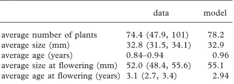
The descriptive properties of the parameterized stochas-tic model can be assessed by calculating the stable size– age distribution numerically and comparing this with the observed data. This shows that there is good agreement between the model and the observed size–age distribution (figure 1). We also calculated various measures of popu-lation size and age structure, using the methods outlined
in Rees & Rose (2002) and Childset al. (2003), and in
all cases the model predictions were in excellent agree-ment with the field data (table 1). As density dependence is explicitly modelled, we can calculate the equilibrium population size, and again there is excellent agreement between the model and the data (table 1).
(b) Fluctuating selection
Recently developed methods for analysing constant-environment integral projection models can be used to quantify the fluctuating selection pressure acting on the
observed flowering strategy (Rees & Rose 2002; Childset
al.2003). We take each year type in turn and assume that
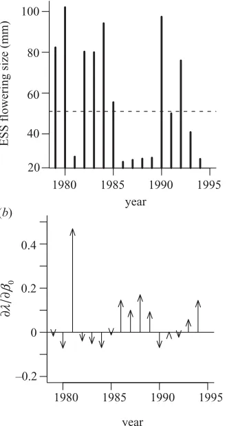
it describes a constant environment inhabited by a popu-lation employing the estimated flowering strategy. Two metrics summarizing the selection acting on the flowering strategy were then calculated for all 16 years: the ESS mean flowering size and the selection pressure on the
intercept of the flowering function (0) (figure 2). The
calculations were carried out assuming that the
size-dependent slope of the flowering function, s, was fixed
at the estimated value. We use this constraint to prevent the ESS strategy being a step function, which occurs as
s→ ⬁ and a=0. The biological motivation for using
this constraint is discussed in § 3c.
The ESS flowering strategy for each year type was
determined by maximizing R0. The year-specific ESS
flowering strategies were highly variable and fall into two broad categories, annual (mean flowering size of less than 30 mm) and delayed reproduction (mean flowering size of
greater than 45 mm) types (figure 2a). The mean
flower-ing size is approximately proportional to⫺0and so
sensi-tivities (∂/∂0) provide an estimate of the selection acting
on the average size at flowering. In half the years, there is
relatively weak selection for larger flowering sizes
(∂/∂0⬍0), whereas in the remaining years there is
much stronger selection for smaller flowering sizes
(∂/∂0≫0).
(c) Evolution of the flowering strategy
We initially calculated the ESS flowering strategy by allowing all three parameters of the flowering function to vary. Under these conditions, we find that the ESS flower-ing strategy tends to a step function with a very small age component (table 2). The predicted average size at flower-ing in this case is greater than the observed value, while the variance in flowering sizes is much lower than in the observed data (figure 3). We recalculated the ESS flower-ing strategy assumflower-ing that the size-dependent slope of the
flowering function,s, is fixed at the estimated value, to
Size-dependent flowering in a variable environment D. Z. Childs and others 429
frequency
1.5 2.0 2.5 3.0 3.5 4.0 4.5 2.0 2.5 3.0 3.5 4.0 4.5
frequency
2.5 3.0 3.5 4.0 4.5
2.0 2.5 3.0 3.5 4.0 4.5
longest leaf length (mm) (log scale)
2.5 3.0 3.5 4.0 4.5 3.0 3.5 4.0 4.5 100
80 60 40 20 0
100 80 60 40 20 0
100 80 60 40 20 0
100 80 60 40 20 0 100
80 60 40 20 0
100 80 60 40 20 0
(a) (c)
(e) (b)
(d) (f)
[image:6.598.52.547.63.244.2]longest leaf length (mm) (log scale) longest leaf length (mm) (log scale)
Figure 1. Observed (solid bars) and predicted (lines) stable size–age distribution for ages 0–5, in (a)–(f), respectively. The bar width in each histogram was chosen using a kernel density estimation routine to make the plots maximally informative.
Table 1. Field data and model predictions. (Values in brackets are 95% confidence intervals.)
data model
average number of plants 74.4 (47.9, 101) 78.2 average size (mm) 32.8 (31.5, 34.1) 32.9 average age (years) 0.84–0.94 0.96 average size at flowering (mm) 52.0 (48.4, 55.6) 55.1 average age at flowering (years) 3.1 (2.7, 3.4) 2.94
growth between when the decision to flower is made and when plant size is measured; (ii) plant size may not be perfectly correlated with the threshold condition for flowering; and (iii) there may be genetic variation in the
threshold condition for flowering. Whensis constrained,
both the mean and variance of the predicted flowering-size distribution are in excellent agreement with the observed data (table 2; figure 3). There is effectively no age component to the ESS flowering function, which is intuitively sensible given that the vital rates are inde-pendent of age.
(d) Fitness landscapes
We generated a fitness landscape in the fully stochastic environment assuming that the resident used the esti-mated flowering strategy (figure 4). Fitness was calculated
for a wide range of0anda, assumingswas fixed. The
ESS strategy lies just outside the 95% confidence envelope
for the estimated parameters. Recall that as0gets smaller
(more negative) so the size at flowering increases. Moving across the landscape from left to right we see a steep increase in the performance of the flowering strategy, which reaches a maximum then declines to a plateau where all strategies have equal fitness. Clearly, flowering at sizes much larger than the ESS results in a dramatic loss of fitness. This is a consequence of high mortality: average-sized plants (32.8 mm) suffer between 15% and 95% mortality, depending on the year type. The plateau in the fitness landscape, corresponding to large values of
0, occurs as all plants adopt the annual flowering
strat-egy, and so have equal performance. Moving vertically across the landscape, we see much smaller changes in
Proc. R. Soc. Lond.B (2004)
performance. This is a direct result of the vital rates being determined by plant size rather than by age.
The pattern of fluctuating selection (figure 2b) can be
understood by examining the fitness landscape (figure 4). We assume that the general topography of the landscape is maintained in different years, though the location of the peak (i.e. the approximate ESS) may vary. In some years, the estimated strategy lies to the right of the peak on the plateau of early-flowering strategies, where there is only weak selection for flowering at larger sizes. In other years, the estimated strategy lies to the left of the ESS on the steep slope of strategies that delay flowering too long. In these instances, there is much stronger selection for flowering at smaller sizes.
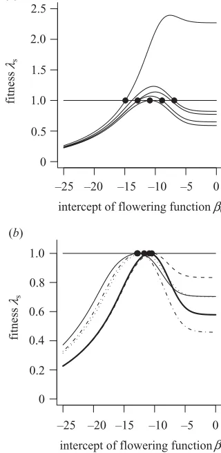
To understand how different sources of variation influ-ence the topography of the fitness surface, we calculated fitness landscapes in constant and stochastic environ-ments. The geometry of a landscape depends in part upon the resident parameter set and not just on the underlying model. To illustrate this, we generated landscapes for five different resident populations in the stochastic
environ-ment, varying the parameter0while fixingsand aat
their estimated values (figure 5a). As the resident
popu-lation moves further away from the ESS the shape and height of the fitness surface are altered. To control for this ‘resident location effect’, we used the environment-specific ESS parameters as the resident parameters when generating landscapes with different sources of temporal variation. Fitness landscapes were generated under five different regimes: a constant environment (using the aver-age number of recruits and the averaver-age intercepts in the survival and growth models; justification for the use of this
model is provided in Reeset al. (2004)), variable
recruit-ment, variable survival, variable growth and the fully stochastic case. The ESS flowering strategy was estimated
by varying only the parameter0. Though the landscapes
have the same general topography, the surface corre-sponding to the fully stochastic model has the sharpest
peak (figure 5b). The largest differences between the
land-scapes occur at small flowering sizes (⫺5⬍0⬍0). In
[image:6.598.50.290.311.397.2]variable-Table 2. Evolutionarily stable flowering strategy in terms of the parameters of the flowering function and the average size and age at flowering, assuming that the slope of the flowering function,s, is constrained at its estimated value and no constraints.
(For reference, the estimated values are also given, values in brackets are 95% confidence intervals.)
parameter mean
size at flowering age at flowering
0 s a (mm) (years)
unconstrained ESS ⫺507 131 ⫺3.50 65.0 2.7
constrained ESS ⫺10.9 — 0.08 51.2 2.5
estimated value ⫺12.1 (⫺9.84,⫺14.26) 2.64 (2.06, 3.22) 0.32 (0.18, 0.45) 52.0 (48.4, 55.6) 2.8 (2.7, 3.4)
1980 1985 1990 1995 40
60 80 100
year
ESS flowering size (mm)
1980 1985 1990 1995 –0.2
0 0.2 0.4
year
∂
∂
0
20 (a)
(b)
β
[image:7.598.55.546.98.196.2]λ
Figure 2. Demonstration of fluctuating selection inCarlina
using (a) ESS flowering size for each year in a constant environment, the dashed line is the observed mean, and (b) selection pressure acting on the intercept of the flowering function,0, in each year.
recruitment environment are much higher, lending sup-port to the idea of a bet-hedging strategy operating in the system. By contrast, early flowering is less costly when sur-vival is variable, because early reproduction reduces the impact of occasional high-mortality years. For large
flowering sizes (0⬍ ⫺10) the effects of stochastic
variation are largely determined by variable survival, as indicated by the close approximation of the variable-survival-only model to the fully stochastic case.
(e) Elasticity and sensitivity analysis
The standard approach for understanding how the vari-ous parameters influence fitness is elasticities analysis. Elasticities can be used to measure the proportional
Proc. R. Soc. Lond.B (2004)
change ins(notthe invasion exponent=logs) caused by
proportional changes inf(t)
a (x,y) and p(
t)
a(x,y).
Tuljapur-kar (1990) presented a numerical method for estimating
the elasticity ofsthat is suitable for matrix models. We
use this approach to generate an approximation for the
elasticity of s to the kernel component functions
kmn(yi,yj), such that
∂logs ∂logkmn(yi,yj)
= lim
T→⬁
1
T
冘
T⫺1
t=0
(v(t⫹1)wT(t))ⴰK˜(t)D
Rtv(t⫹1)w(t⫹1)
, (3.1)
where the mandnsubscripts refer to the kernel
compo-nent function in themth row andnth column ofK˜(t), and
ⴰ denotes the Hadamard operator. The terms w(t) and
v(t) satisfy
w(t⫹1)=K˜ (t)Dw(t)
Rt
and vT(t⫺1)=v
T(t)K˜(t⫺1)D
Qt ,
(3.2)
where Rt=储K˜(t)w(t)D储 and Qt=储vT(t)K˜(t⫺1)D储 (see
Caswell 2001, p. 402). Justification for the use of this approach is given in Appendix A. As elasticities sum to unity, this analysis allows us to partition the contributions
off(t)
a(x,y) and p(
t)
a(x,y) tosof different age classes. We
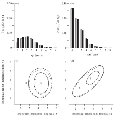
also calculated elasticities for a constant-environment model (using the average number of recruits and the aver-age intercepts in the survival and growth models). The elasticity surfaces corresponding to the constant and stochastic environments are almost identical (figure 6). They show that the survival–growth function makes a
larger contribution tosthan does the fecundity function
(constant environment, 0.70 and 0.30, respectively; stochastic environment, 0.67 and 0.33, respectively) and
that the largest contributions toscome from changes in
the survival–growth function, p(t)
a(x,y), of young plants.
4. DISCUSSION
We have shown how the integral projection model may be used to explore the demography and evolution of size-and age-structured populations in a density-dependent stochastic environment. The resultant model combines the flexibility of the individual-based approach with the computational efficiency and power of traditional matrix methods. However, unlike parameterization of age- and size-structured matrix models (Law 1983), parameteriz-ation of the integral projection model is straightforward
and requires no new techniques beyond standard
[image:7.598.89.254.229.539.2]Size-dependent flowering in a variable environment D. Z. Childs and others 431
longest leaf length (mm) (log scale)
frequency
3.0 3.5 4.0 4.5 80
60
40
20
[image:8.598.72.272.58.237.2]0
Figure 3. Observed distribution of flowering sizes (solid bars) and predictions from the various models. The bold line is the fitted model, the dotted line is from the unconstrained ESS model and the solid thin line is from the constrained ESS.
2
1
0
–1
–2
–25 –20 –15 –10 –5 0 0.8
0.6
0.4
0.2
0.8 1.0
0.9
age slope of flowering function
a
β
intercept of flowering function β0
Figure 4. The fitness landscape forCarlina, calculated assuming that the resident population uses the estimated flowering strategy in a fully stochastic environment. The filled point is the estimated flowering strategy, and the bold ellipse is the 95% confidence contour, calculated using the standard quadratic approximation to the likelihood— assuming that the likelihood is2-distributed with three degrees of freedom. The open point is the ESS prediction assumingsis fixed.
simple field data, we were able to make very accurate
pre-dictions of the distribution of flowering sizes in Carlina.
Invasibility analysis reveals that the observed flowering strategy is close to the ESS and that temporal variation in recruitment, growth and survival are all important influ-ences on the evolutionarily stable flowering size (figure 5).
These results reinforce the conclusions of Rees et al.
(1999) and Roseet al.(2002) on the need to include
tem-poral variation in life-history studies.
The parameterized model provides an accurate descrip-tion of the number of individuals and the distribudescrip-tion of
Proc. R. Soc. Lond.B (2004)
–25 –20 –15 –10 –5 0 0
0.5 1.0 1.5 2.0 2.5
intercept of flowering function 0
fitness
s
–25 –20 –15 –10 –5 0 0
0.2 0.4 0.6 0.8 1.0
intercept of flowering function 0
λ
β
β
(a)
(b)
fitness
s
[image:8.598.342.502.71.399.2]λ
Figure 5. Fitness landscapes as a function of0, the intercept of the flowering function: (a) stochastic environ-ment with five different residents, (b) different variable environments with the environment-specific ESS as the resident strategy (thick line, fully stochastic environment; thin line, constant environment; dotted line, variable growth only; dashed line, variable survival only; dotted–dashed line, variable recruitment only).
sizes within each age class, the distribution of flowering sizes, average age at reproduction and average population size. Clearly, an adequate model must at least describe the data well if it is to be used to draw further conclusions.
However, a parameterized model of Carlina ignoring
stochastic variation failed to predict the mean and variance of the ESS flowering distribution, while still providing an
accurate description of the population structure (Childset
al. 2003). By contrast, the stochastic model presented
here predicts an evolutionarily stable flowering size (51.2 mm) that is very close to the estimated mean size at flowering (52.0 mm), provided that the variance in the threshold size distribution is constrained. Interestingly, in
the constant-environment case (Childs et al. 2003), the
parameters of the constrained ESS are not significantly different from the estimated parameters of the flowering function, yet the fitness difference between the estimated
and evolutionarily stable flowering functions wasca. 10%.
Conversely, in the stochastic model the ESS parameters are significantly different from the estimated parameters,
though the fitness difference is only ca. 2%. Taken
together, these observations indicate that an adequate
description of the life history of Carlinaneeds to include
[image:8.598.53.294.309.532.2]age (years)
∂
ln
(
λs
)
∂
ln
(
fa
)
longest leaf length (mm) (log scale) t
longest leaf length (mm) (log scale)
t
+ 1
longest leaf length (mm) (log scale) t
0.30
0.20
0.10
0
0 1 2 3 4 5 6 7 8
age (years)
0 1 2 3 4 5 6 7 8
6
5
4
3
2
6
5
4
3
2
2 3 4 5 6 2 3 4 5 6
0.30
0.20
0.10
0
(a) (b)
(c) (d)
0 6
0
6
∂
ln
(
λs
)
∂
ln (
pa
[image:9.598.107.486.56.441.2])
Figure 6. Elasticity analysis of the kernel component functions in constant (grey bars, dashed lines) and stochastic (black bars, continuous lines) models. Elasticity values summed over size for (a)fa(x,y) and (b) pa(x,y) for all ages. Elasticity contour plots for (c)fa(x,y) and (d) pa(x,y) for ages 0 and 6, showing the 0.000 003 contour for each age.
need to be careful when comparing the predictions of evolutionary models with data, as different metrics may produce different results. It is also important to dis-tinguish between biological significance (measured in terms of fitness differences) and statistical significance when making such comparisons.
The fitness landscapes (figure 5b) have well-defined
maxima in contrast to those of several other studies (Klinkhamer & de Jong 1983; Tuljapurkar 1990), and the sharpness of the peak increases as different forms of stoch-asticity are included in the model (figure 5). This discrep-ancy between our study and earlier studies is probably a result of exploring models with several forms of stochas-ticity. The importance of different sources of stochasticity depends on flowering size; in large flowering plants, fitness is primarily determined by fluctuations in survival, whereas in small flowering ones fluctuations in recruit-ment are critical. Thus, the generalization of Caswell (2001), that in stochastic environments fitness optima are often flat, may be a consequence of including only a single form of stochasticity in earlier models.
Selection and common garden experiments have shown
that natural populations harbour extensive genetic
variation for flowering size (reviewed in Metcalf et al.
2003). The mechanisms responsible for the maintenance
Proc. R. Soc. Lond.B (2004)
of this variation are not known but theoretical work has shown that an evolutionarily stable population has a posi-tive genetic variance maintained by selection providing that the product of the variance of fluctuations, the amount of generation overlap and the selection intensity is sufficiently high (Ellner & Hairston 1994). This
mech-anism could operate in Carlina as there is fluctuating
selection (figure 2b) and overlapping generations.
Elasticity analysis was used to partition contributions to
sfrom different kernel component functions, age classes
and sizes. In this system the survival–growth functions
make a greater contribution tosthan the fecundity
func-tions, because reductions in growth and survival of a parti-cular age class reduce opportunities for reproduction in
subsequent years. Younger plants contribute most to s
because they represent a larger proportion of the stable age distribution. However, this underlying trend is tem-pered by the fact that younger, and hence smaller, plants contribute relatively few recruits to the next generation
(figure 6a,b). Elasticity contour plots for the fecundity
functions demonstrate that contributions to s through
recruitment are most important for large individuals,
whiles is influenced by the survival of a wide range of
size types (figure 6c,d). Individuals are, on average, larger
Size-dependent flowering in a variable environment D. Z. Childs and others 433
high-density regions of the elasticity surfaces toward larger sizes for older age classes. As found in several other stud-ies, the constant-environment elasticities provide an excel-lent approximation to the stochastic-environment ones (Benton & Grant 1996; Caswell 2001).
By combining techniques for the modelling of size- and age-dependent demography in a stochastic environment with ideas from evolutionary demography we have been
able to show that the observed flowering strategy in
Car-linais close to the ESS and that accurate prediction of the
distribution of flowering sizes is possible. What is not clear is how different forms of stochasticity influence the ESS. There are two distinct ways in which temporal variation could be important. First, when the environment varies through time, average demographic rates differ from demographic rates in the average environment owing to nonlinear averaging. Second, the ESS will vary from year to year, owing to non-equilibrium dynamics. Methods for quantifying the relative importance of different forms of stochasticity and how nonlinear averaging and non-equilibrium dynamics contribute to this are explored in Reeset al. (2004) where techniques for decomposing the effects of stochastic selection are developed.
APPENDIX A: STOCHASTIC GROWTH RATE AND SENSITIVITY ANALYSIS
We supply some technical details for the C. vulgaris
model; more general models will be considered elsewhere. As in the corresponding deterministic model (appendix to
Childs et al. 2003), some special model properties allow
derivations based on matrix-model theory:
(i) all living individuals have some probability of repro-ducing now or later;
(ii) there is a maximum possible age,m; and
(iii) the size distribution of new offspring (age=0) is the
same for all parents in all years:
fd(x,y)=0(y), (A 1)
with the environment states(t) determining the
sur-vival and growth functions and the total number of recruits each year.
As a result of (ii) and (iii), after an initial transient of, at
most, myears the state of living individuals is a function
only of the environment states ‘now’ and over the pastm
years, (t)=((t),(t⫺1),%,(t⫺m)). Consider
indi-viduals now of some agea.
(i) One component of (t) determines the number of
recruits Rt⫺a in their year of birth, and thus
deter-mines the initial cohort asn0(x,t⫺a)=Rt⫺a0(x).
(ii) Other components of (t) then determine the
sur-vival and growth functions that act on this cohort in each subsequent year up to the present.
Thus, the entire resident population state at timetis a
det-erministic function of the random environment process
(t).
By assumption, the environment states (t) are
independent and identically distributed, hence (t) is a
stationary ergodic first-order Markov chain. The resident-population process is therefore stationary and ergodic
(with stochastic growth 0, neither increasing nor
decreasing). Its numerical properties can be determined either by simulation and averaging, or by numerically
Proc. R. Soc. Lond.B (2004)
implementing the population-dynamic iterations (using
the (t)-dependent kernel components) that generate the
current population state as a function of(t).
An invader’s population dynamics are density inde-pendent with equations (2.9) and (2.15) giving the fec-undity (survival and growth are density independent for both resident and invader). All terms in these equations
are functions of(t), either directly or via the dependence
of the resident-population state on (t). The invader is
therefore governed by a stochastic density-independent integral projection model in which all components depend
on (t). However, this can be reduced to a stochastic
matrix model for the total number of individuals in each age class, implying the existence of a stochastic growth rate, as follows.
As with the resident, after a possible transient of length
mall individuals of agesj⬎0 are descended from a cohort
with size distribution 0 and therefore have size
distri-butions proportional toj(y,t) where
j⫹1(y,t⫹1)=
冕
⍀
j(x,t)p(jt)(x,y)dx,
j⫹1=j⫹1
冒
冕
⍀
j⫹1dy. (A 2)
The fraction surviving to agej⫹1 is therefore
Pj(t)=
冕
⍀
冕
⍀j(x,t)p(jt)(x,y)dxdy. (A 3)
Note that, since 0 is independent of time, equation
(A 2) constructs j(y,t) as a function of (t), hence
Pj(t) is a function of (t). Similarly, the per capita
fec-undity of age-j individuals is
Fj(t)=
冕
⍀
冕
⍀j(x,t)f(jt)(x,y)dxdy. (A 4)
As noted above,f(t)
j is determined by(t), soFj(t) is also
determined by (t). The population count vector
N(t)=[N0(t),N1(t),%,Nm(t)], consisting of the total
numbers in each age class, therefore satisfies a stochastic
Leslie matrix L(t) having the same form as the K˜(t)D
matrix (equations (2.6) and (2.7)),
N(t⫹1)=
冢
F0(t) F1(t) % Fm⫺1(t) Fm(t)
P0(t) 0 % 0 0
⯗ P1(t) ⯗ ⯗
⯗ ...
0 0 % Pm⫺1(t) 0
冣
N(t).
(A 5)
The random matrix sequence L(t) is stationary and
erg-odic, and its values lie in an ergodic set (there are
16m⫹1 possible values of (t) each generating a possible
value ofL(t), and all have the same incidence matrix which
is power-positive). The fact that the set of values ofL(t)is
finite also implies that Emax{0,log储L(t)储} is finite, hence
standard results for stochastic matrix models (see
The elasticity analysis (equations (3.1) and (3.2)) depends on two additional properties (see Tuljapurkar
(1990), § 11.2). First, the process(t) generating the vital
rates can be run backwards in time by running(t)
back-wards in time, which is possible since values of(t) are
gen-erated independently over time. Second, the reduction to a matrix model above implies that the growth rate is a smooth function under perturbations of the matrix (and hence under perturbations of the integral model kernel components that generate the matrix). Equations (3.1) and
(3.2) therefore give the elasticity of theapproximate
stochas-tic growth rate generated by the quadrature approximation
to the stochastic integral model (i.e. theK˜(t)D matrix). In
other words, by formally reducing the model to equation (A 5) we have shown that the stochastic growth rate exists and has well-defined elasticities. The calculations in § 3e
involving the K˜(t)D matrix are a straightforward way to
obtain approximate numerical values of these quantities (to any desired accuracy, by increasing the number of mesh points) using standard matrix operations and software.
REFERENCES
Benton, T. G. & Grant, A. 1996 How to keep fit in the real-world: elasticity analyses and selection pressures on life-histories in a variable environment.Am. Nat.147, 115–139. Caswell, H. 2001Matrix population models. Construction,
analy-sis and interpretation. Sunderland, MA: Sinauer Associates.
Charlesworth, B. 1994 Evolution in age-structured populations. Cambridge Studies in Mathematical Biology. Cambridge University Press.
Childs, D. Z., Rees, M., Rose, K. E., Grubb, P. J. & Ellner, S. P. 2003 Evolution of complex flowering strategies: an age-and size-structured integral projection model approach.
Proc. R. Soc. Lond. B270, 1829–1838. (DOI 10.1098/
rspb.2003.2399.)
Cole, L. C. 1954 The population consequences of life history phenomena.Q. Rev. Biol.29, 103–137.
de Jong, T. J., Klinkhamer, P. G. L., Geritz, S. A. H. & van der Meijden, E. 1989 Why biennials delay flowering—an optimization model and field data on Cirsium vulgare and
Cynoglossum officinale.Acta Bot. Neerland.38, 41–55.
de Jong, T. J., Klinkhamer, P. G. L. & de Heiden, J. L. H. 2000 The evolution of generation time in metapopulations of monocarpic perennial plants: some theoretical consider-ations and the example of the rare thistle Carlina vulgaris.
Evol. Ecol.14, 213–231.
Easterling, M. R. 1998 The integral projection model: theory, analysis and application. PhD thesis, North Carolina State University, Raleigh, NC, USA.
Easterling, M. R., Ellner, S. P. & Dixon, P. M. 2000 Size-specific sensitivity: applying a new structured population model.Ecology81, 694–708.
Ellner, S. & Hairston, N. G. 1994 Role of overlapping gener-ations in maintaining genetic variation in a fluctuating environment.Am. Nat.143, 403–417.
Eriksson, A. & Eriksson, O. 1997 Seedling recruitment in semi-natural pastures: the effects of disturbance, seed size, phenology and seed bank.Nordic J. Bot.17, 469–482. Kachi, N. & Hirose, T. 1985 Population dynamics of
Oeno-thera glaziovianain a sand-dune system with special
refer-ence to the adaptive significance of size-dependent reproduction.J. Ecol.73, 887–901.
Klinkhamer, P. G. L. & de Jong, T. J. 1983 Is it profitable for biennials to live longer than two years? Ecol. Model. 20, 223–232.
Proc. R. Soc. Lond.B (2004)
Klinkhamer, P. G. L., de Jong, T. J. & Meelis, E. 1987 Delay of flowering in the biennialCirsium vulgare: size effects and devernalization.Oikos49, 303–308.
Klinkhamer, P. G. L., de Jong, T. J. & Meelis, E. 1991 The control of flowering in the monocarpic perennialCarlina vul-garis.Oikos61, 88–95.
Klinkhamer, P. G. L., de Jong, T. J. & de Heiden, J. L. H. 1996 An eight-year study of population dynamics and life-history variation of the ‘biennial’Carlina vulgaris.Oikos75, 259–268.
Law, R. 1983 A model for the dynamics of a plant population containing individuals classified by age and size.Ecology64, 224–230.
Metcalf, J. C., Rose, K. E. & Rees, M. 2003 Evolutionary demography of monocarpic perrenials.Trends Ecol. Evol.18, 471–480.
Metz, J. A. J., Nisbet, R. M. & Geritz, S. A. H. 1992 How should we define ‘fitness’ for general ecological scenarios?
Trends Ecol. Evol.7, 198–202.
Mylius, S. D. & Diekmann, O. 1995 On evolutionarily stable life histories, optimization and the need to be specific about density dependence.Oikos74, 218–224.
Rees, H., Childs, D. Z., Rose, K. E. & Grubb, P. J. 2004 Evol-ution of size-dependent flowering in a variable environment: partitioning the effects of fluctuating selection.Proc. R. Soc.
Lond.B271. (In the press.) (DOI 10.1098/rspb.2003.2596.)
Rees, M. & Rose, K. E. 2002 Evolution of flowering strategies
in Oenothera glazioviana: an integral projection model
approach. Proc. R. Soc. Lond. B269, 1509–1515. (DOI 10.1098/rspb.2002.2037.)
Rees, M., Sheppard, A., Briese, D. & Mangel, M. 1999 Evol-ution of size-dependent flowering inOnopordum illyricum: a quantitative assessment of the role of stochastic selection pressures. Am. Nat.154, 628–651.
Rees, M., Mangel, M., Turnbull, L. A., Sheppard, A. & Briese, D. 2000 The effects of heterogeneity on dispersal and colon-isation in plants. In Ecological consequences of environmental
heterogeneity (ed. M. J. Hutchings, E. A. John & A. J. A.
Stewart), pp. 237–265. Oxford: Blackwell Scientific. Rees, H., Childs, D. Z., Rose, K. E. & Grubb, P. J. 2004
Evol-ution of size-dependent flowering in a variable environment: partitioning the effects of fluctuating selection.Proc. R. Soc. Lond. B271. (In the press.) (DOI 10.1098/rspb.2003. 2596.) Roff, D. A. 1992The evolution of life histories. Theory and
analy-sis. London: Chapman & Hall.
Rose, K. E., Rees, M. & Grubb, P. J. 2002 Evolution in the real world: stochastic variation and the determinants of fit-ness inCarlina vulgaris.Evolution56, 1416–1430.
Sletvold, N. 2002 Effects of plant size on reproductive output and offspring performance in the facultative biennialDigitalis purpurea.J. Ecol.90, 958–966.
Stearns, S. C. 1992The evolution of life histories. Oxford Univer-sity Press.
Tuljapurkar, S. 1990 Population dynamics in variable
environ-ments. Lecture Notes in Biomathematics. London: Springer.
Venables, W. N. & Ripley, B. D. 1997Modern applied statistics
with S-PLUS. New York: Springer.
Weiner, J., Martinez, S., Muller-Scharer, H., Stoll, P. & Schmid, B. 1997 How important are environmental maternal effects in plants? A study withCentaurea maculosa.
J. Ecol.85, 133–142.
Wesselingh, R. A., Klinkhamer, P. G. L., de Jong, T. J. & Boorman, L. A. 1997 Threshold size for flowering in differ-ent habitats: effects of size-dependdiffer-ent growth and survival.
Ecology78, 2118–2132.