White Rose Research Online URL for this paper:
http://eprints.whiterose.ac.uk/3383/
Article:
Sumalee, A. (2007) Multi-concentric optimal charging cordon design. Transportmetrica, 3
(1). pp. 41-71. ISSN 1812-8602
[email protected] https://eprints.whiterose.ac.uk/
Reuse
See Attached
Takedown
If you consider content in White Rose Research Online to be in breach of UK law, please notify us by
Universities of Leeds, Sheffield and York
http://eprints.whiterose.ac.uk/
Institute of Transport Studies
University of Leeds
This is the publisher produced version of an article originally printed in
Transportmetrica. The copyright is held by the publishers and this version has
been uploaded with their express permission.
White Rose Repository URL for this paper:
http://eprints.whiterose.ac.uk/3383
Published paper
Sumalee, A. (2007) Multi-concentric optimal charging cordon design.
Transportmetrica, 3(1), pp.41-71.
41
MULTI-CONCENTRIC OPTIMAL CHARGING CORDON DESIGN
AGACHAI SUMALEE1
Received 30 March 2006; received in revised form 29 October 2006; accepted 29 October 2006
The performance of a road pricing scheme varies greatly by its actual design and implementation. The design of the scheme is also normally constrained by several practicality requirements. One of the practicality requirements which is tackled in this paper is the topology of the charging scheme. The cordon shape of the pricing scheme is preferred due to its user-friendliness (i.e. the scheme can be understood easily). This has been the design concept for several real world cases (e.g. the schemes in London, Singapore, and Norway). The paper develops a methodology for defining an optimal location of a multi-concentric charging cordons scheme using Genetic Algorithm (GA). The branch-tree structure is developed to represent a valid charging cordon scheme which can be coded using two strings of node numbers and number of descend nodes. This branch-tree structure for a single cordon is then extended to the case with multi-concentric charging cordons. GA is then used to evolve the design of a multi-concentric charging cordons scheme encapsulated in the two-string chromosome. The algorithm developed, called GA-AS, is then tested with the network of the Edinburgh city in UK. The results suggest substantial improvements of the benefit from the optimised charging cordon schemes as compared to the judgemental ones which illustrate the potential of this algorithm.
KEYWORDS: Road pricing, charging cordon design, optimal toll problem, genetic algorithm
1. INTRODUCTION
The concept of road pricing emerged from the idea that the cost paid by the road user (called marginal private cost or perceived cost) is actually lower than the actual cost he or she imposes (called marginal social cost) (Pigou, 1920; Knight, 1924; Walters, 1961; Vickrey, 1963). Thus, by imposing an appropriate toll level on travellers, additional social welfare improvement can be gained. Based on this simple economic theory, several researchers have been attempting to analyse the setting of appropriate toll level in the real world situation in which transport system has to be treated as a network. However, most of these works mainly focused on the theoretical part of the toll design and particular paid attention only on the toll level not the toll location problem.
May et al. (2002) pointed out several practical design criteria of a road pricing scheme. Particularly, some key characteristics of a practical road pricing scheme found are related to the topology of charging points. It is widely believed that a charging cordon is the most user-friendly charging system due to its simplicity and clarity to the road users. This is considered to be a key ingredient for promoting public acceptability of the charging scheme. A charging cordon is a set of tolled links surrounding a designated area so that all trips entering or passing through that area are tolled. Various current real world implementations of the scheme including the ERP scheme in Singapore, Norwegian toll rings (in Oslo, Trondheim, and Bergen), and the congestion charging scheme in London.
The common practice in designing a charging cordon scheme documented in various real-world cases and desk studies (May, 1975; Holland and Watson, 1978; Transpotech, 1985) is to apply a judgmental approach or a ‘trial and error process’ to seek appropriate toll locations and toll levels. The trial and error process normally starts by defining a set of possible charging cordons and their associated common toll levels. Then, each option is tested with some traffic modelling software. The benefit and cost of
1
each scheme is then calculated from the modelling output and the best scheme from those considered is chosen.
The sub-optimality of this judgmental design approach is well addressed in May et al. (2002) in which the benefits of cordons based on the judgmental and optimal designs are compared. They also suggested that the application of a theoretical approach could improve the benefit of the judgmental design significantly. One possibility is to directly optimise the location of charging cordons using optimisation theory. The motivation of this paper is to develop an optimisation method to find optimal locations specifically for charging cordons.
Recently, there have been an increasing number of attempts to develop analytical approaches to tackling the optimal toll level and location problems (Mun et al., 2001; Hearn and Yildirim, 2002; Hyman and Mayhew, 2002; May et al., 2002; Verhoef, 2002; Ho et al., 2005; Lawphongpanich and Hearn, 2004; Shepherd and Sumalee, 2004; Zhang and Yang, 2004). Most of the literature concentrates on deriving the solution of optimal toll level and location without considering the topological constraint of the charging scheme. Only some of the research considered the requirement for a charging cordon. Mun et al. (2001), Hyman and Meyhew (2002), and recently Ho et al. (2005) developed approaches to define the optimal location of a charging cordon with a non-network based modelling framework (using either a continuum traffic model or strategic model).
However, the omission of network representation in the model may cause a sub-optimal design of the cordon location. There are two particular reasons; firstly congestion is a local issue which happens mostly on links rather than in wide areas; secondly the analysis of charging scheme without a network representation may underestimate the impact of re-routing (Milne, 1997). Thus, it is considered more appropriate to tackle the cordon design problem under the framework of network modelling.
Zhang and Yang (2004) developed an approach based on ‘genetic algorithms’ (GA) to find an optimal closed charging cordon with an optimal uniform toll under a detailed network representation. The method proposed later on in this paper was independently developed based on a similar principle, with GA being utilised as the main optimisation mechanism.
The difference between the method in this paper and the one in Zhang and Yang (2004) is largely in the chromosome design (which is the proxy for a charging cordon in GA). Their chromosome represents the status of nodes, identifying whether they are tolled or tolled. From a set of tolled and tolled nodes, the links starting from one of the un-tolled nodes and ending at one of the un-tolled nodes are defined as un-tolled links. They also proposed a method to verify whether a set of tolled links forms a charging cordon. However, this chromosome design does not ensure that after the crossover or mutation operators are applied the new chromosome will represent a charging cordon. On the other hand, the method in this paper ensures that the new chromosomes conserve the closed charging cordon formation after the GA operators are applied. In addition, the chromosome structure proposed in this paper can be extended easily to the case with multi-concentric charging cordon scheme. This paper extends the formulation proposed in Sumalee (2004) by including the general case of the multi-concentric charging cordon scheme. A multi-concentric cordon is a scheme with a number of charging cordons all of which share the same centre and all the cordons do not overlap each other. Further explanation is given later in Section 5.1.
defining a set of charging cordons. The third section introduces the concept of GA and explains the detail of GA-AS. Section four then presents an extension of the method to the design of a multi-concentric charging cordon scheme. Section five investigates the influence of different GA parameters by testing GA-AS with the Edinburgh network. The last section summarises the paper.
2. OPTIMAL CHARGING CORDON DESIGN PROBLEM
The problem discussed in this paper is to find the optimal location of tolled links forming a charging cordon or multiple charging cordons, with their optimal toll levels, designed to maximise or minimise a selected objective function (e.g. social welfare improvement, total travel time, accessibility, or local environmental improvement).
2.1 Notation
I the set of OD-pairs, denoted i = 1, …, I
Ti the continuous number of users (or OD-flow) for OD pair i, with Ti ≥ 0
Di(Ti) the continuous differentiable inverse demand function for trips for OD-pair i, with Di ≤ 0
J the set of directed links in the network
vj the continuous number of users (or link flow) on link j, with Vj ≥ 0
cj(vj) the strictly monotone differentiable average cost function excluding tolls for the use of link j, with cj ≥ 0
εj A dummy that takes on the value of 1 if a toll can be charged on link j, and a value of 0 otherwise
sj the cost of implementation and operation of a tolled link τj the level of the toll on link j if εj = 1
i,j,P index for OD pairs, links, and paths respectively
2.2 Mathematical program of optimal charging cordon scheme design
In this paper, the problem is limited the case of single user class, single mode, and with elastic demand. The rational road users’ response is assumed to follow Wardrop’s user equilibrium, UE (Wardrop, 1952). In analysing the optimal toll design problem, this UE condition has to be imposed as one of the constraints in the optimization problem. The second important constraint is that the selected toll links must form a charging cordon. Let Θ be the set of all possible multi-concentric charging cordon schemes. A feasible combination of tolled links for the optimisation problem must be one of the members of this set,ε ∈ Θ. With these two constraints, the general problem of optimal charging cordon design can be formulated as:
(
)
maxψ F, ,τ ε (1a)
subject to
( )
(
)
sol UE
→ τ
F , (1b)
U ≤ τ ≤ ε
0 , (1c)
{ }
0,1ε ∈ , (1d)
where F is a vector of path flows and F→sol UE
(
( )
τ)
means that the flows must be the user’s equilibrium flow given the toll vector. The constraint 0≤ τ ≤ εj U j is included toensure that a toll is not imposed on a link which is not selected as a tolled link
(
ε =j 0)
.Withε =j 0, 0≤ τ ≤j 0and hence τj must be equal to zero. The implementation of U
is to allow the toll of a tolled link
(
ε =j 1)
to be any value between0≤ τ ≤j U . U can bean arbitrary “large” number or a specified upper bound of possible toll level.
This problem aims to find a combination of toll points (also find the number of toll point) forming a multi-concentric charging cordon scheme and its uniform toll level of each cordon so that it maximize the objective function of ψ which can be either social welfare benefit or revenue. The traditional economic objective of optimal road pricing design is to maximise the ‘net benefit’ which is the social welfare benefits minus the costs of the road pricing system (i.e. implementation and operation costs). For the social welfare benefits, a social surplus measure will be used (‘Marshallian measure’). There are two components in measuring the social surplus, consumer surplus and consumer cost. The gross total benefit can be mathematically formulated as:
( )
( )
0 i
T
i j j j j j
i j j
D x dx c v v s
ψ =
∑
∫
−∑
−∑
ε (2)The first and second terms are the consumer surplus and consumer cost respectively. The net of these two values is the social welfare (or social surplus). The third term is the cost of the road pricing scheme. In the optimisation problem discussed in this paper, the objective function of the program is to maximise the net benefit compared to the benefit in the do-nothing scenario (no toll). This objective can be seen as the objective to increase the efficiency of the transport system.
This problem can be categorised as a Mathematical Program with Equilibrium Constraints (MPEC). There are various problematic characteristics of MPEC, e.g. non-convex feasible regions, non-non-convex objective functions, and non-smooth objective functions. Solving the MPEC problem is a very complicated task, let alone the combinatorial nature of the problem stated earlier. In addition, it is infeasible to handle the constraint on the topology of tolled links (due to its complexity) with the traditional optimisation algorithms.
To author’s knowledge, there does not exist any derivative-based optimisation algorithm that is capable of solving this problem. In this paper, the idea to tackle this problem is to utilise the flexibility of GA in dealing with the constraint of a multi-concentric charging cordon scheme and the UE condition. GA is first used to produce a set of charging cordons. The users’ responses, following users’ equilibrium, to the cordon toll are then evaluated by running an appropriate traffic assignment model. The fitness of each closed cordon will be evaluated from the users’ responses. GA will then iteratively evolve the set of charging cordon solutions until reaching the predefined stopping criteria (e.g. maximum number of generations within GA).
3. BRANCH-TREE FRAMEWORK FOR REPRESENTING A CHARGING CORDON
3.1 Definition of a charging cordon
Definition 1: Charging cordon. A charging cordon is a set of tolled links surrounding a designated area so that all private car users travelling to the destination inside the area or through the area will be charged. A definition of a closed cordon in the context of graph theory is that all paths from all zones outside the cordon passing through the nodes inside the cordon must be tolled at least once on a link related to those paths.
Zhang and Yang (2004) defines a charging cordon based on the concept of a cutset in graph theory. It is worthwhile to reiterate the concept proposed in their paper in order to distinguish the differences between the methods developed in this paper and their method.
Definition 2: Cutset. For a directed graph G = (N, A), a cutset of G is a subgraph consisting of a minimal collection of links whose removal reduces the rank of G by one.
Definition 3: Component. A component of a graph is a connected subgraph containing the maximal number of edges. If a graph is not strongly connected, it must contain a number of components. Otherwise, a graph has only a single component.
Assumption 1: In this paper, only a complete directed graph is considered which means there is only one component of the network. In other words, there is at least a path connecting each pair of nodes in the network.
Definition 4: Incident matrix. An incident matrix (B) with the dimension of N×A is a representation of a graph (G) where the elements of the matrix (bn a, ) are defined as follows:
,
1 if node is the origin node of link 1 if node is the destination node of link 0 otherwise
n a
n j
b = −⎧⎪⎨ n j
⎪⎩ (3)
Lemma 1: For a graph with N nodes and β components, the rank of the graph (γ) is
defined as the number γ =N− β = the number of linearly independent rows or columns of the incident matrix (B) of G.
Theorem 1 [Zhang and Yang, 2004]: Given a graph representing a road network and a cutset, tolled links forming a charging cordon are those whose original node is in the component outside the cutset and destination node is in the component inside the cutset.
Proof. From Assumption 1, the graph considered is complete, so it only has one component. A set of links forming a cutset reduces the rank of the matrix by one and only one (due to Definition 2) which means it will increase the number of components of the graph by one and only one. This is true because the number of nodes in the graph before and after applying the cutset is constant and from Lemma 1 γ =N− β. Thus, the links forming a cutset will split the network (graph) into two components. By putting the tolls on all links heading toward the component inside the cutset all paths entering this area are charged which satisfies the definition of a closed charging cordon in Definition 1.
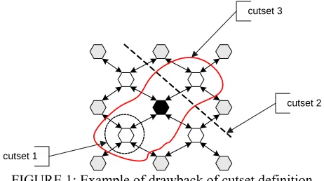
the set of charged nodes. From this condition, cutset 1 satisfies the standard condition for a cutset but it does not form a desired charging cordon surrounding the desired charging area.
cutset 2
cutset 1
[image:8.499.134.365.117.246.2]cutset 3
FIGURE 1: Example of drawback of cutset definition
However, although the condition on the charged nodes is imposed (i.e. the central node is defined as the charged node), cutset 1 and cutset 2 shown in Figure 1 still satisfy the condition for a cutset and charged node. The remedy for this problem is to include an additional constraint on the other set of nodes (referred to as boundary nodes). Boundary nodes and charged nodes must be in different components of the graph. From Figure 1, if an additional constraint on boundary nodes is imposed, neither cutset 1 nor cutset 2 satisfies this condition since some of the boundary nodes and charged nodes are in the same components of the graph. Cutset 3, on the contrary, satisfies this condition and this cutset forms a charging cordon according to Definition 1.
The method proposed in Zhang and Yang (2004), thus, could experience this drawback. In addition, the GA chromosome design in their method may not form a new charging cordon after the GA operators are applied to the chromosomes. The branch-tree approach proposed next overcomes these two drawbacks. The branch-tree concept does naturally conform to the requirement in Definition 1. The next section explains the concept of a branch-tree approach for defining a charging cordon.
3.2 Nomenclature of the branch-tree concept
Let G = (N, A) be a directed graph representing an urban traffic network where N and
A are a set of nodes and links respectively in the graph. A link is defined by two nodes, i
and j where i≠ j i j; , ∈N.
Definition 5: Set of all preceding nodes. If the direction of a link is from i to j, i is termed ‘the preceding node’ of j. The number of preceding nodes for each node j can be more than one. The set Ξ =j
{
i iis the preceding node of j}
is defined to be the set of‘all-preceding nodes’ of node j where Ξj is the size of the set (the total number of
preceding nodes of node j).
Definition 6: Node degree. The degree of a node is the number of children or preceding nodes of that node in the branch-tree.
Definition 8:Branch-tree and Branching process.β =r
{
( , )n d}
is a branch-tree, which is defined as a set of the pairs of n, n∈N and d (degree of node n). r is the root node of this branch-tree (r∈N). β =r{
( , )n d}
has to be created from the original graph G. Given G, a root node (r) is defined and then only the preceding nodes of r can be included into the branch-tree, i.e. n can be included into the branch-tree if and only ifr
n∈ Ξ (See Definition 5).
When node n is added into the branch-tree, the degree of node n is initially set as zero (since node n has no children nodes in the branch-tree at this stage). Node n can then be expanded by including its preceding nodes into the branch-tree. The set of preceding nodes of node n added into the branch-tree are referred as children nodes of node n. After adding the preceding nodes of node n into the branch-tree, the degree of node n
will be changed from zero to the number of children nodes of node n. This is the process to expand the ‘depth’ of the branch-tree which is referred to as the ‘branching process’. The branching process can be applied iteratively to other leaf nodes added into the branch-tree. Once the process terminates, β =r
{
( , )n d}
is produced. Example 1 below illustrates the branch-tree structure and branching process. [image:9.499.161.319.410.594.2]Example 1 Illustration of the branching process
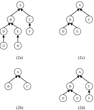
Figure 2a shows an example of a full traffic network (G). Assume that node A is defined as root node β =A
{
(A, 0)}
. According to Definition 5 given earlier, nodes B and C are the preceding nodes of node A and they can be added into the branch-tree βA. Figure 2b shows the branch-tree after applying the branching-process to node A (adding nodes B and C into the original branch-tree shown in Figure 2b). At this stage{
}
A (A, 0), (B, 0), (C, 0)
β = . Notice that the degree of node A is changed from zero to two (see Definition 8 above). Nodes B and C are now the leaf nodes of the branch-treeβA.
A
B C
D E
G H
F
(2a)
A
B C
(2b)
A
B C
D E
(2c)
A
B C
D E F
(2d)
Assume that only node B will be expanded. Nodes D and E which are the children nodes of node B are added into the branch-tree during the branching process creating the new branch-tree as shown in Figure 2c. At this stage,
{
}
A (A, 0), (B, 0), (C, 0), (D, 0), (E, 0)
β = . Again, notice the change of the degree of node B from zero to two. If the branching process is terminated at this stage, the final branch-tree βA is the one shown in Figure 2c. Applying the branching process to expand the depth of the branch-tree with different set of leaf nodes can create different branch-trees from the same graph (see Figure 2d for a different branch-tree from the graph in Figure 2a where the branch-tree is also expanded at node C).
Definition 9: Sub-branch. Recall that β =r
{
( , )n d}
is a branch-tree. Given n which is one of the nodes in β =r{
( , )n d}
, β ⊂ βn r is a sub-branch of βr. Inside a branch-tree, a number of sub-branches can be defined. Assume that node n from a full branch-tree is selected, the sub-branch created from this node is the whole part of the branch-tree rooted from node n. Figure 3 shows an example of a sub-branch rooted from node B of the full branch-tree shown in Figure 2c. In this example node B from the branch-tree (βA) shown in Figure 2c is selected as the root node of the sub-branch. βB, which is a sub-branch of the branch-tree, is thus the whole part of the branch-tree rooted from node B which are node D and E. Therefore, β =B{
(B, 2), (D, 0), (E, 0)}
and thus β ⊂ βB A.B
D E
FIGURE 3: Example of sub-branch
Definition 10: Branch. Given a branch-tree β =r
{
( , )n d}
and its associated original graph G, a branch is defined as a linka
∈
A
defined by a leaf node of β =r{
( , )n d}
as its origin node and a proceeding node of that branch node in β =r{
( , )n d}
as its destination node. For example, from the branch-tree shown in Figure 2d, the branches of this branch-tree are links D-B, E-B, and F-C.3.3 Relationship between branch-tree and closed charging cordon
After introducing the necessary notation for the branch-tree concept, this section explains how a branch-tree can represent a closed cordon scheme.
Proposition 1: For a given branch-tree (β =r
{
( , )n d}
), the tolled links are defined by a set of branches in the branch-tree. These tolled links will form a closed charging cordon around the root note r if and only if all nodes in β =r{
( , )n d}
have either d = 0 ord= Ξn . This implies that in expanding a leaf node (using the branching process) all preceding nodes of that leaf node must be included into the branch-tree. This is exactly the process adopted in the example in Figure 2.
the branch-tree, all links entering that leaf node will be defined as tolled links and hence all paths entering that (previously) leaf node are tolled. From a root node (r), by including all preceding nodes of the root node into the branch-tree all paths entering that root node are tolled. In expanding the leaf node j (which are all preceding nodes of node
r), from the proposition all preceding nodes of node j (∀n n| ∈ Ξj) must be included into the branch-tree. Note that now all paths entering node j must pass through one of the preceding nodes of node j. By tolling the links defined by node j and its preceding nodes all paths entering node j are tolled. Previously, all paths entering node r via node j are tolled by the tolled link (r, j). After expanding node j, the new set of tolled links ensuring that all paths entering node j are tolled and hence all paths entering node r via node j are still tolled. This proof can be expanded to the general case between node j and j+1 where node j+1 is one of the children nodes of node j, hence it proves that the condition of a branch-tree proposed is sufficient for defining a charging cordon according to Definition 1.
Before generating different charging cordons, a set of predefined links forming an initial charging cordon in the network must be defined. The starting node of each link will become a root node for the branch-tree. For instance, assuming that in a network the predefined cordon comprises five links, five branch-trees will be generated to define the set of charging cordons. These five branch-trees generated from the predefined cordon can be combined into a single global branch-tree with a given virtual root node reducing five branch-trees to a single branch-tree which represents a charging cordon.
Example 2 Relationship between branch-trees and charging cordons
Figure 4a shows the hypothetical network used for exemplification. The grey node is assumed to be the city centre which is the preferred tolled area. In a network, as mentioned earlier a set of links forming an initial closed cordon around the tolled area must be predefined. Assume that Cordon 1 in Figure 4a is defined to be the initial cordon. From this initial cordon, a virtual root node (name “C1”) is defined for the branch-tree, and the first level nodes in the branch-tree are the preceding nodes of the links forming the initial cordon (Cordon 1). Figure 4b shows the branch-tree C1 representing the initial cordon.
Assume that node E is to be expanded to create a new cordon. The original branch-tree in Figure 4b is then expanded at node E, creating the new branch-tree as shown in Figure 4c. This new branch-tree forms Cordon 2 shown in Figure 4a. In Figure 4d, the original branch-tree is instead expanded at node G to produce Cordon 3. All three cordons in Figure 4a are closed cordons. The tolled links in each cordon are defined by the branches in the branch-trees. Note that nodes E-L, which are predefined by the user, are referred to as ‘target nodes’ because they are the set of nodes where all paths passing through these nodes must be tolled. The branching process will be applied to each target node in turn to define the shape of the cordon, as illustrated in Figure 4. This notation will be used in the algorithm for generating a closed charging cordon in the next section.
Next, several issues related to the structure of a branch-tree and conventional rules for branching process will be discussed.
3.4 Dummy nodes in a branch-tree
C1
E F G H I J K L
D A
B
C E
G
K
I F
L J
H
M
T
S R
Q P O
N
C1
E F G H I J K L
C1
E F G H I J K L
M T
N O
(4a)
(4b)
(4c)
(4d) Cordon 1
[image:12.499.96.399.77.321.2]Cordon 2 Cordon 3
FIGURE 4: Relationship between branch-trees and charging cordons
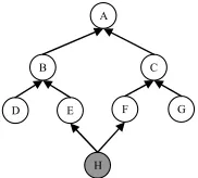
Definition 11: Dummy node. For a given branch-tree, a node with more than one acceding nodes in the branch-tree is referred to as a dummy node.
Example 3 Dummy nodes example
Figure 5 illustrates this problem where node H has two acceding nodes, i.e. nodes E and F, and hence there are two possible paths to traverse between nodes A and H in the branch-tree. Let βB and βC be two sub-branches of branch in Figure 5. If β ∩ β ≠ ∅B C ,
then βBand βCare referred to as non-separable sub-branches. This means sub-branches
B
β and βC must have some overlapping parts (nodes) (see Figure 5). There must be at least one common node (θ) appearing in both sub-branches,
( )
θ,d ∈ β ∩ βB C. These nodes are named ‘dummy nodes’such as node H in Figure 5.
A
B C
D E F G
H
[image:12.499.192.283.507.589.2]Dummy nodes will be expanded in only one sub-branch in order to avoid the inconsistency in the structure of the cordon. In order to do this, we establish rules for expanding the branch as follows:
Algorithm 1:
Step 1: Check if there is θ (dummy node) in the branch-tree, if true go to Step 2, otherwise continue branching process as described in Section 3.2.
Step 2: For each θ, check if θ in all sub-branches are leaf nodes; if so go to Step 3. Otherwise go to Step 4.
Step 3: Label θ as “Dθ” and put θ on the branch with zero degree as normal. The reason for re-labelling dummy nodes is to hint to the crossover and mutation process in GA that changing this node involves other dummy nodes in the branch. Finish the process.
Step 4: Label node θ as “Dθ”. Then put “D” as the node degree for the node in the sub-branch that will not be expanded. For the node in the sub-sub-branch that will be expanded, operate the branching process as explained earlier.
3.5 Two-way link issue
Links and nodes in a graph, G = (N, A), represent roads and junctions in a road network. For a two-way link defined by node i and j, node i is a preceding node of node j and vice versa. As mentioned, in the branching process a leaf node, n, can be expanded by including all nodes in Ξn into the branch-tree resulting in the change of the node degree
from zero to Ξn . Assume that a leaf node n is expanded from node j. In fact, node j is one of the preceding nodes of node n due to its two-way link property. If node n is to be expanded, node j should not be included into the branch-tree again. If node j is included into the branch-tree, the toll will be imposed on the traffic coming from inside the cordon.
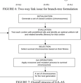
Example 4 Two-way links in general traffic network
Figure 6 is used to illustrate the issue of two-way links. Figure 6a is the road network used in this example. Note that the link between nodes A and B is a two-way link. The original branch-tree is shown in Figure 6b where the tolled links are links (B, A) and (D, A). Node A is used to represent the area inside the charging cordon defined by the branch-tree. Assume that the branch-tree is to be expanded at node B that has both nodes A and C as its preceding nodes. In this case, only node C will be added into the branch-tree, which represents link (C, B) (see Figure 6c). Node A will not be added into the branch-tree again. If node A were added into the branch-tree, link (A, B) would be defined as a tolled link. The toll on link (A, B) would then be imposed on the traffic coming from node A which is the traffic from inside the cordon. In the general process of building a branch-tree or in the branching process, there is a process to detect this two-way link issue to avoid tolling traffic coming out from inside the charging cordon.
4. APPLYING GA TO SOLVE THE OPTIMAL CLOSED CORDON
defined by ‘population numbers’) representing a set of charging cordons encapsulated in the form of chromosomes (using the branch-tree formulation). Then, in the ‘Evaluation’ process for each cordon an optimal cordon toll is found by testing it with different pre-specified tolls. Each toll level is implemented in the network, and then a traffic modelling software package, in this case, SATURN (Van Vliet, 1982), is used to predict the responses of road users to the toll. The net total benefit from each toll level is calculated from the modelling outputs. The toll level producing the highest net total benefit is then selected as the optimal uniform toll for that cordon. It should be noted that any other traffic modelling software or even different equilibrium paradigms (e.g. stochastic equilibrium) could be used with the method described in this paper so long as it is able to produce the outputs required for the calculation of the net total benefit.
B D
A
A B
C
D
B D
A
C
[image:14.499.136.365.214.293.2](6-6a) (6-6b) (6-6c)
FIGURE 6: Two-way link issue for branch-tree formulation
INITIALISATION
Generate a set of closed cordons (chromosomes)
EVALUATION
Test each cordon with predefined tolls and identify an optimal uniform toll and related benefits (fitness) for that cordon
SELECTION
Select survival chromosomes based on their fitness
GA OPERATORS
Apply crossover and mutation process to survival chromosomes
A set of chromosomes for the next generation
FIGURE 7: Overall process of GA-AS
[image:14.499.121.380.275.540.2]The chromosome design in GA-AS for closed cordons associated with the branch-tree concept is discussed next. The algorithm (based on recursive programming) to generate the initial set of charging cordons is then described. Next, the selection process, which is based on the method of roulette wheel linked with the linear ranking method proposed by Whitley (1989), is explained. Then, the two important genetic operators used in this method, i.e. crossover and mutation, are discussed.
4.1 Chromosome design
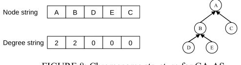
It is crucial to design a chromosome structure that is compatible with the structure of the branch-tree explained in the previous section. More importantly, the chromosome structure should be able to maintain the feasibility of the solution (in this case, the closed cordon format) even after applying the crossover and mutation process. As mentioned in the previous section, the members of a branch-tree have two key characteristics, i.e. their node numbers and degrees. Therefore, two strings, each a series of numbers or alphabets, will be used to represent a chromosome. The first string, called the node string, contains the node numbers of the branch-tree. The second string, called the degree string, contains the degree of each node in the corresponding column in the node string. Figure 8 shows an example of a chromosome.
A
B C
D E
A B D E C
2 2 0 0 0
Node string
[image:15.499.113.360.314.381.2]Degree string
FIGURE 8: Chromosome structure for GA-AS
The node string tells us that this branch-tree comprises nodes A, B, D, E, and C. The degree string tells us that nodes A, B, D, E, and C have the degrees of 2, 2, 0, 0, and 0 in that order. This chromosome represents the branch-tree shown in Figure 2c. However, from the node and degree strings, the only information provided is which nodes are in this branch-tree and the degrees of each node. They do not provide any information about the connection of the nodes in the branch-tree. For example, how may one know that node B is the preceding node of node A without looking at Figure 2c? The answer is in the order of the nodes in the node string. The algorithm for encoding a chromosome from a branch-tree explains the meaning of the node sequence in the node string. The algorithm used to encode the branch-tree to node and degree strings is as follows:
Algorithm 2:2
Step 1: Set k to be the first column in node and degree string. Set j equals to 1. Put the root node and its degree into column k.
Step 2: Set Pj = a set of all preceding nodes of the node in k. Set Pj = ∅.
Step 3: Check if Pj =Pj. If so, set j = j –1 and then go to Step 7. Otherwise go to Step 4.
Step 4: Set k = k+1.
2
Step 5: Set nj to be a node in Pj but not in Pj. Put nj into the k column of node string
Step 6: Put the degree of nj into the k column of degree string. Add nj to Pj. If degree of
nj is equal to zero, go to Step 3. Otherwise set j = j+1 and go to Step 2. Step 7: Check if j = 0. If so, stop. Otherwise, go to Step 3.
Example 5 Demonstration of encoding a branch-tree into a chromosome format for GA-AS
From Figure 8, first node A is put into the first column of the node string and its degree (2) is put into the first column of the degree string. Then set P1=
{ }
B, C which is the set of all preceding nodes of node A. In Step 5, node B is picked and placed in the second column of the node string. In Step 6, the degree of node B, which is two, is placed into the second column of the degree string and node B is added into P1. Since the degree of node B is not equal to zero, j is set equal to 2 and we then go to Step 2. In Step 2, we set{
}
2 D, E
P = and in Step 3 node D is picked and put into the third column of the node string. Also, the degree of node D, which is 0, is put into the third column of the degree column. Node D is also added into the set P2. Since the degree of node D is zero, the process moves straight to Step 3.
In Step 3, since
{
D, E} { }
≠ D , node E is picked and the same process is repeated as node D (the degree of node E is also null). The process returns to Step 3 again, and this time P2=P2 ={
D, E}
. Thus, j is set to 1, and the process moves to Step 7 and then Step 3 sequentially (since j≠0). Since{ } { }
B, C ≠ B , node C is picked and put in the fifth column. Again, its degree, which is zero, is put in the fifth column of the degree string. Now, P1={ }
B, C =P1. Therefore, in Step 3, j is set to zero and the process is terminated.4.2 Initialisation
In this stage, a number of charging cordons are randomly generated. The number of cordons generated in the first generation of the GA is controlled by the pre-defined population numbers. The generation of a closed cordon is designed as a random process. The variable ‘Prop’ is defined as the probability of a node to be expanded (recall the definition of branching process explained earlier). The user must also define the initial closed cordon by defining a set of tolled links. The preceding nodes of these links will become a set of target nodes (see Figure 4). The initialisation process is as follows:
Algorithm 3:
For each target node defined by the user
Step 1: Set k to be the first digit in the node and degree string. Set j equal to 1. Put the root node and its degree into column k.
Step 2: Set
k
j n
P = Ξ (a set of all preceding nodes of the node in k). Set Pj = ∅.
Step 3: Check if Pj =Pj. If so, set j = j –1 and then go to Step 9. Otherwise go to Step 4.
Step 4: Set k = k+1.
Step 6: Use algorithm 6-1 to check dummy nodes and check the issue of two-way links Step 7: Add nj to Pj. If nj is a dummy node or representing the link in the opposite
direction (two-way link issue), then go to Step 3. Note that if nj is ignored due to the two-way link issue, remove that node from Pj . Otherwise, go to Step 8.
Step 8: Generate a random number (rand). If rand > Prop, then put Pj as the degree of
nj into the k column of the degree string; and then set j = j+1 and go to Step 2. Otherwise, the degree of nj is equal to zero (put “0” into the k column of the degree string); go to Step 3.
Step 9: Check if j = 0. If so, stop. Otherwise, go to Step 3.
As mentioned, in the previous section, there may be some issues over the dummy nodes and two-way links. These issues are considered in Step 6.
4.3 Evaluation process
Once the chromosome is generated, the next task is to evaluate its fitness. The fitness is measured according to the objective function which is the net total benefit. There are two possible strategies, grid-search for optimal toll and binary toll vector.
4.3.1 Grid-search strategy
In order to evaluate the objective function, the optimal toll level for each cordon (chromosome) must be defined. Since finding the optimal toll level involves solving the optimisation problem, the process of evaluating the exact benefit of each chromosome can be very time consuming. Instead, in this method the simple uniform toll regime is assumed in order to ease the evaluation process. This assumption is also consistent with the judgmental design criteria mentioned earlier. Initially, a set of predefined toll levels is defined e.g. 100, 200, and 300 pence. For the test in this paper, eight toll levels are defined which are £0.50, £0.75, £1.00, £1.25, £1.50, £2, £3 and £4. Each chromosome (representing a charging cordon) will be evaluated with each toll level. The toll level producing the highest objective function (net total benefit) will be chosen as the optimal uniform toll for that chromosome which gives the fitness (objective function) of that chromosome.
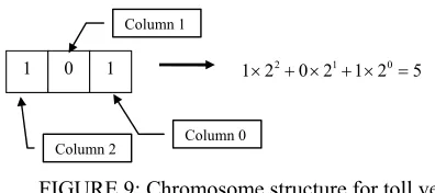
4.3.2 Toll-vector strategy
1 0 1 1 2× 2+ × + ×0 21 1 20=5
[image:18.499.133.331.73.161.2]Column 2 Column 0 Column 1
FIGURE 9: Chromosome structure for toll vector
4.4 Selection process
The selection process used in GA-AS is based on ‘stochastic universal sampling’ which uses a single wheel spin (Michalewicz, 1992). The so called ‘roulette wheel’ is constructed where each slot represents a chromosome. In the original form of the roulette wheel, the slots are sized according to the fitness of each chromosome, which represents the probability of a chromosome being selected. However, since the fitness value (total benefits minus scheme costs) in the optimal cordon problem can be negative (which causes a problem for allocating the space for each chromosome on the wheel) the linear ranking approach proposed by Whitley (1989) is adopted. The slots in the roulette wheel are sized according to the chromosome at rank i, where the first is the best chromosome, by the following equation:
1
2 (2 2) 1
i
P i
p c c
P P
⎛ ⎛ − ⎞⎞
⎜ ⎟
= ⎜ − + − ⎜⎜ ⎟⎟⎟
−
⎝ ⎠
⎝ ⎠
(4)
where P is the size of the population (set P), and 1≤ ≤c 2 is the ‘selection bias’: higher values of c cause the system to focus more on selecting only the better chromosomes. The strongest chromosome in the population can thus be selected with the probability of c P/ ; the weakest chromosome can be selected with the probability of
(2−c) / P . After each chromosome is assigned its probability to be selected, the next step is to calculate a cumulative probability (qi) for each chromosome:
1
i
i j j
q =
∑
= p (5)Each time, a chromosome is selected for a new population by generating a random number r from the range [0..1]. If r < q1 the first chromosome is selected; otherwise
select the i-th chromosome such that qi−1< <r qi. Indeed, some chromosomes would be selected more than once according to the selection probability of each chromosome. As part of the selection process, the idea of ‘elitism’ is also adopted to ensure that the best chromosome in the current generation will be included in the population of the next generation.
4.5 Crossover process
The complication involved in crossing the chromosomes in GA-AS is the strict structure of the branch-tree. The process has to start by identifying identical nodes in two mated branch-trees. Then, the crossing node is randomly chosen from the set of identical nodes. The parts of node and degree strings representing the sub-branches in two mated branches rooted from the chosen node are identified. Then, the two sub-branches are crossed over to produce two new chromosomes. Example 6 and Figure 10 illustrate this process.
Example 6 Illustration of crossover process for the branch-trees
From Figure 10, there are two original mated branch-trees (in Figure 10 a and Figure 10b). The set of common nodes in these two mated chromosomes (except root node) are nodes B, C, D, E, F, and G. Assume that node C is randomly selected by the crossover process. The sub-branches rooted from node C in two branch-trees are identified which are the parts inside the dash-line boxes in Figure 10a and Figure 10b. These two branches in the two mated chromosomes are then switched. In other words, the sub-branch in the line box in Figure 10a is moved to replace the sub-sub-branch in the dash-line box in the other branch-tree in Figure 10b, and vice versa. Figure 10c and Figure 10d show the two new branch-trees after crossover.
A
B C
D E F G
I
A
B C
D E F G
H J K L
A
B C
D E F G
I J K L
A
B C
D E F G
H
(10a) (10b)
[image:19.499.144.385.282.491.2](10c) (10d)
FIGURE 10: Crossover process for branch-tree
The existence of a dummy node requires the algorithm to check the new chromosome after the crossover operation. After applying GA operators, an algorithm for detecting the new dummy nodes as the result of the crossover operation must be applied to the new chromosomes.
4.6 Mutation process
The second GA operator is the mutation process which aims to preserve the diversity amongst the population and to represent the stochastic evolution process in nature. In a typical mutation process, the value of the bit to be mutated in the string will be changed to the opposite value, i.e. if the current value is “1” then it will be changed to “0” and vice versa. However, the chromosome structure in GA-AS is not consistent with the traditional binary string chromosome. Thus, a new approach to mutate the chromosome is developed. The mutation process in GA-AS involves the branching process at a node (including both branching in and out). For a leaf node, if the node is to be mutated, the node will be expanded following the branching process explained earlier (this is the branching out process). Alternatively, if the node to be mutated is not a leaf node, the branch-tree will be branched in at that node, i.e. converting that node to a leaf node and removing all nodes below the mutated node from in a sub-branch. Example 7 and Figure 11 illustrates how the mutation works.
Example 7 Illustration of the mutation process for branch-tree
The branch-tree in Figure 11c is used as the original branch-tree in this example. The two branch-trees in Figure 11a and Figure 11b exhibit the mutation as branching in where node F is contracted. In this example, nodes J and K are removed from the branch-tree as the result of the mutation at node F; the degree of node F is also set to zero. The two branch-trees in the lower part demonstrate the branching out as the mutation process where node I is expanded. Nodes M, N, and O which are the preceding nodes of node I in the full network are added to the branch-tree; the degree of node I is also changed to three.
A
B C
D E F G
I J K L
A
B C
D E F G
I L
A
B C
D E F G
I J K L
A
B C
D E F G
I J K L
M N O
(11a) (11b)
[image:20.499.102.366.357.590.2](11c) (11d)
FIGURE 11: Mutation process for branch-tree
process, the normal GA mutation method can be applied directly to the toll string if GA-AS is asked to optimise the uniform toll level as well.
5. GA-AS FOR MULTI-CONCENTRIC CHARGING CORDON SCHEME DESIGN
In some cases, a charging cordon scheme may comprise a set of charging cordons. By introducing additional cordons, the tolls imposed on each trip can be better adjusted according to its length, contribution to congestion, externalities generated, etc. The GA-AS method proposed in the previous section and the concept of branch-tree framework proposed in Section 3 can be extended to deal with the multi-concentric cordon design problem. This section explains the approach to extend GA-AS for this problem. The extended method is named GA-ASII.
5.1. Required condition for multi-concentric charging cordons
Definition 12: Multi-concentric cordons. There is a restriction on the design of the multiple charging cordon schemes. Let Ci denotes charging cordon i where i∈
{
1,…,n}
.1
C is defined as the narrowest cordon and Cn as the widest cordon. Let Li be the set of links covered inside the cordon Ci. The restriction of the shape of the multiple cordon scheme adopted in this chapter is that Li ⊂Li+1. This condition ensures that the narrower cordon i is completely located inside the next wider cordon (cordon i+1).
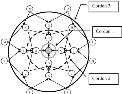
Example 8 Multi-concentric cordons
Figure 12 illustrates the meaning of this condition. From Figure 12, cordon 1, which is the narrowest cordon (or the most inside cordon), is completely inside cordon 2. Similarly, cordon 2 is completely inside cordon 3, which is the widest cordon. This shape of multi-concentric cordons scheme facilitates the extension of the branch-tree framework to this problem and it is also consistent with the idea of simple scheme design which enhances the practicality of the scheme.
D A
B
C E
G
K
I F
L J
H
M
T
S R
Q P O
N Cordon 3
[image:21.499.156.367.431.594.2]Cordon 2 Cordon 1
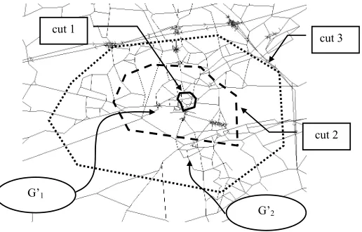
5.2 Hyper-graph approach to define multiple charging cordons
As mentioned, the desired topology of multiple charging cordon design explained in the previous section allows a straightforward extension of the branch-tree framework to representation of multiple charging cordons. The strategy is to divide the original network, G, into a number of sub-networks (denoted as Gk′) as shown in Figure 13. The network will be divided by a series of cuts, denoted as rk. The area between two cuts (rk and rk+1) represents a desired area for putting a charging cordon Ck. Recall that an initial cordon must be given to define a set of charging cordons (see Section 3). For area
k
G′, the ring rk will be used as the initial cordon for cordon Ck.
cut 3
cut 2 cut 1
G’1
[image:22.499.123.381.209.374.2]G’2
FIGURE 13: Defining multiple charging cordons with cuts
For each Gk′ a branch-tree concept explained earlier can be used directly to define a charging cordon in that area. In addition, this partition approach ensures that the multiple-charging-cordon scheme satisfies the requirement declared in the previous section. Figure 13 illustrates the partition approach.
The set of cuts adopted to partition the network are cuts 1, 2, and 3 as shown in the figure. Cuts 1 and 2 define G1′ which is the area for the first cordon, C1 (the narrowest cordon). In addition, cut 1 is the initial cordon for the generation of a charging cordon in
1
G′.
5.3 GA implementation
5.3.1 Chromosome structure
The chromosome structure for a single cordon design is comprised of two strings: node string and degree string (as explained earlier). In the MCD problem, two strings are needed for representing each cordon. Therefore, in finding K optimal cordons (Ck for k
= 1, …, K) a number of strings needed for one chromosome is 2K. The chromosome of a multi-layer cordon scheme in the MCD problem is thus a collection of K chromosomes of single cordons. Figure 14 shows an example of a chromosome for the MCD problem (with three charging cordons).
A B E D F
2 2 0 0 0
G K R S L
2 2 0 0 0
P U T N M
2 2 0 0 0
Cordon 1 Cordon 2 Cordon 3
[image:23.499.128.374.189.285.2]One chromosome
FIGURE 14: Chromosome structure for multiple charging cordons
With the new chromosome structure, the initialisation, crossover, and mutation process explained earlier can be applied to each pair of node and degree strings.
5.3.2 Evaluation
Different toll levels may be allowed for different cordons. One strategy to find an optimal combination of toll levels is to test a multiple cordon scheme with all possible combinations of tolls. This strategy is suitable for the problem with a low number of charging cordons and possible toll levels (e.g. for two cordons with three possible toll levels, the number of possible toll combinations is only nine). However, the number of possible toll combinations can be increased dramatically with the number of cordons and possible toll levels on each cordon. For example, with two cordons and six possible toll levels on each cordon the number of possible toll combinations is 36.
An alternative approach, toll-vector strategy, discussed earlier, which optimises both toll level and cordon location simultaneously, offers a more convenient implementation of GA-AS with the MCD problem. For each solution, a toll string (binary number string) representing the toll level of a cordon is associated with each cordon in that solution. In the case where all cordons will have the same toll level, only one toll string is required. The crossover and mutation process can be applied to these toll strings directly. Given the natural extension of the toll string approach to the MCD problem, GA-ASII will adopt the toll-vector strategy.
6. TESTS WITH THE EDINBURGH NETWORK
(Oscar Faber, 2001). If we assume a 30 year life, a discount rate of 6% and 1000 peak hours per year then this is approximately equivalent to £100 per toll point per peak-hour. The tests conducted in this section are as follows:
(i) Use GA-AS with grid-search to find optimal cordon and uniform toll (ii) Use GA-AS with toll vector to find optimal cordon and uniform toll
(iii) Use GA-ASII with and without toll vector to find double cordons with two toll levels.
[image:24.499.112.387.255.404.2]6.1 Comparison between GA-AS with grid-search and toll-vector
Figure 15 shows the Edinburgh network with three judgmental cordons. The three judgmental cordons were designed following the judgmental criteria discussed in May et al. (2002). The inner cordon 2 is used as the initial cordon for GA-AS and the ring road is used to define the boundary of the charging cordon. The optimal uniform toll level and its associated social welfare benefit were found for each judgmental cordon (see Table 2).
Outer cordon
Inner cordon 1
Inner cordon 2
FIGURE 15: Edinburgh network and three judgmental charging cordons
GA-AS with grid-search and with toll-vector are then applied to find an optimal cordon and its associated optimal uniform toll. Table 1 shows the parameters used for both algorithms (the number of modelling runs are limited to be the same for both methods). Note that for each chromosome GA-AS with grid-search needs eight SATURN runs to find its associated benefit. Figure 16 shows the comparison of the plot of the best objective function found so far against the number of modelling runs for GA-AS with the grid-search and toll-vector. The total CPU-time for a run of GA-GA-AS (given the number of generations and population) is around three hours.
TABLE 1: Parameters used for GA-AS
Population number Generation number Probability of crossover
Probability of mutation
Number of elitism chromosomes
50 200 0.75 0.15 5
grid-search strategy, a chromosome with a lower objective function (associated with its optimal toll) is less likely to survive compared to the case with the toll-vector strategy. For example, with the grid-search a chromosome i is pooled with n other chromosomes. Assume that other chromosomes (representing different cordons) have substantially higher objective functions with their associated optimal tolls (found from grid-search) compared to the objective function of chromosome i. In this case, the probability of chromosome i to be selected would be very low. On the other hand, with the toll-vector approach, although chromosome i is pooled with the same n chromosomes, it may have a higher probability to survive if the toll vectors of n other chromosomes produce lower objective functions compared to the toll vector of chromosome i.
4000 4500 5000 5500 6000 6500 7000 7500
0 1000 2000 3000 4000 5000 6000 7000 8000
Number of runs
Soci
al w
e
lf
a
re
improv
ement of optimal s
o
lution found so far
(pounds/pea
k hour)
[image:25.499.103.391.203.376.2]GA-AS with toll-vector GA-AS with grid-search
FIGURE 16: Performance comparison between GA-AS with grid-search and toll-vector strategies
The relationship of this phenomenon with the searching mechanism of GA is that GA-AS with the grid-search will have a more limited searching space compared to the searching space of GA-AS with toll-vector. It is well known in theory of GA that some weaker chromosomes may lead the searching algorithm to a better chromosome. Therefore, by associating the fitness of each cordon to its optimal toll the algorithm may lose some weaker cordons whose topology may lead the algorithm to the optimal or better solution. In addition, GA-AS with grid-search may waste too much computational time in applying the grid search without associating the solutions with the crossover and mutation processes which are the search operators for GA.
Figure 17 and Figure 18 show the actual distribution of the fitness of the chromosomes from GA-AS with toll-vector and grid-search respectively. The comparison of these two figures demonstrates the advantage of using GA-AS with the toll-vector strategy in terms of the diversity of the solution and searching space. Note that despite a smaller number of plots of the population on Figure 18 for GA-AS with the grid-search strategy, the number of simulation runs in both cases is equal.
optimise both cordon location and toll level. However, it should be noted that this analysis is only limited to one case and the results may be vary from case to case.
-50000 -40000 -30000 -20000 -10000 0 10000
[image:26.499.126.373.109.254.2]0 2000 4000 6000 8000 10000
FIGURE 17: Fitness distribution of GA-AS with toll-vector
-50000 -40000 -30000 -20000 -10000 0 10000
[image:26.499.127.367.289.443.2]0 2000 4000 6000 8000
FIGURE 18: Fitness distribution of GA-AS with grid-search
6.3 Optimal cordon without a constraint on toll level
6.3.1 Maximise social welfare improvement
Figure 19 shows the optimal cordon solution found with the toll level of £1.50. The cordon solution found has 13 tolled links (highlighted links).
FIGURE 19: Optimal cordon solution found by GA-AS
The optimal toll found for OPC1 is £1.50 which is considered a reasonable level of toll. In fact, the current plan of the congestion charging in Edinburgh considers the implementation of £2 double toll rings. It is interesting to see the sensitivity of the net benefit of the scheme when the toll is varied. Figure 20 shows the net benefit and revenue curves of the OPC1 with eight different toll levels adopted during the optimisation process.
Figure 20 confirms the optimal toll level found by GA-AS with toll vector (approximately £1.50) and shows that the benefit of the cordon varies significantly with the toll level. Unsurprisingly, if the objective function is to maximise the revenues, the optimal toll level for OPC1 could be well beyond £4 observing from the revenue curve in Figure 20.
-4000 -2000 0 2000 4000 6000 8000
0 50 100 150 200 250 300 350 400 450
Toll level (pences)
G
ross
to
ta
l benef
it
(
£
/p
eak hour
)
0 10000 20000 30000 40000 50000 60000 70000 80000 90000 100000
R
evenu
es (
£/
p
eak
hou
r)
[image:27.499.104.399.406.585.2]Gross total benefit Revenues Poly. (Revenues) Poly. (Gross total benefit)
Apart from the best cordon found so far (OPC1), during the GA-AS optimisation process we also can identify the cordons producing the second and third highest net total benefit (named OPC2 and OPC3 respectively). Figure 21 shows the location of OPC2 and OPTC and Table 2 shows the net total benefit and optimal toll level of these two cordons.
Different toll points from OPC1
Different toll points from OPC1
OPC2
[image:28.499.157.343.144.409.2]OPC3
FIGURE 21: Cordons with 2nd and 3rd highest net total benefits
TABLE 2: Summary of the results of designing a single optimal charging cordon for Edinburgh network
Charging system Optimal toll No. of toll points
Cost (£k/hour)
Revenue (£k/hour)
Total benefit (£k/hour)
Net total benefit (£k/hour)
Net revenues (£k/hour) Inner cordon 1 £0.50 9 0.90 12.60 3.00 2.10 11.70 Inner cordon 2 £0.75 7 0.70 18.40 4.69 3.99 3.99 Outer cordon £0.75 20 2.00 22.20 3.96 1.96 1.96 OPC1 £1.50 13 1.30 45.10 8.51 7.21 43.70 OPC2 £1.50 14 1.40 45.00 8.51 7.11 43.60 OPC3 £1.50 14 1.40 45.10 8.50 7.10 43.70 OPC-REV £4.00 32 3.20 111.10 -45.99 -49.19 107.90 D-OPC £1.25, £1.25 38 3.80 105.30 19.08 15.28 101.50
[image:28.499.71.429.465.570.2]OPC2, and OPC3 are almost identical (around £8.51k/peak hour). Thus, the higher net benefit of OPC1 is mainly due to a smaller number of toll points. It is interesting that a charging cordon with a smaller number of toll points (like OPC1) is capable of generating the same or even higher benefit compared to OPC2 and OPC3. This re-confirms the importance of careful selection of the location of charging cordons and toll points.
6.3.2 Maximise net revenues
[image:29.499.122.385.334.522.2]The objective being optimised in the previous subsection is the net total benefit. In this section, GA-AS is used to optimise the net revenues instead (using the same GA parameters as shown in Table 1). Figure 22 shows the best cordon and uniform toll level found for maximising the revenues. The optimal toll level for this charging cordon is £4, as expected. This charging cordon is named OPC-REV. OPC-REV consists of 32 toll points which is substantially higher than the number of toll points of OPC1. Table 2 shows the main result of the test with OPC-REV. From the result, OPC-REV generates approximately £111.1k /peak hour. On the other hand, it also causes substantial negative impact in terms of the social welfare (with £-41.19k / peak hour of social welfare disbenefit). A combination of the high number of charging point, high toll level, and a wide range of the coverage of the routes in the network enables OPC-REV to generate such a high revenues.
FIGURE 22: Location of OPC-REV (maximise net revenues)
6.3 Multiple cordons design
strategy for optimising double toll levels. The parameters adopted for GA-ASII in the test are the same as presented earlier in Table 1.
[image:30.499.129.377.239.412.2]Figure 23 shows the locations of optimal double charging cordons found by GA-ASII. Although the toll levels were allowed to vary between the two cordons, the optimal uniform tolls found for the inner and outer cordons are both £1.25. The net benefit from this double cordon (D-OPC) is around £15.3k per peak hour which is more than double the net benefit of OPC1. The inner and outer cordons are comprised of nine and 29 toll points respectively giving the total number of toll points of 38. The revenue generated from D-OPC is about 5% lower than the revenue of OPC-REV. Figure 24 shows the surface of the net total benefit of D-OPC when the toll levels on the inner cordon and outer cordon are varied. The optimal tolls for inner and outer cordons from the surface are both £1.25. Differentiating the tolls on two cordons did not bring in additional benefit. Note that this result is only specific to this network and may not be true in other cases.
[image:30.499.120.379.441.606.2]FIGURE 23: Optimal double charging cordons for the Edinburgh network
6.4 Overall comparison
This section summarises the results from all the tests explained earlier. Table 2 presents the key performance indicators for all the tests conducted. As explained, there are four different sets of results. The first group is the test with the judgmental design (inner cordon 1, inner cordon 2, and outer cordon). The second test is the optimal single cordon design maximising the objective function of net total benefit (OPC1, OPC2, and OPC3). The third is the optimal single cordon design but with the objective of maximising the net revenue (OPC-REV). The final test is to find the optimal double charging cordon maximising the net total benefit (D-OPC).
As explained earlier, the cordons designed by applying GA-AS outperform the judgmental design. The improvement of the benefit from the careful design is approximately 80% better than the performance of the best judgmental design. The optimal toll level for the optimised design is around £1.50 whereas the optimal uniform toll for the judgmental cordons is around £0.50 - £0.75. Introducing the second cordon, D-OPC, obviously increases the performance of the charging cordon scheme. The benefit generated by D-OPC is around 110% higher than the benefit from OPC1. In terms of the net revenues, as expected, OPC-REV generates the highest net revenues even when compared to the D-OPC. However, this comes with a substantial trade-off with the net total benefit of the scheme.
7. CONCLUSIONS
Based on the review, one of the most practical designs of a road pricing scheme is a charging cordon. This presents a challenge in devising a sounding method for aiding the practitioner in locating the best location of a cordon charging scheme. This paper presents a method based on Genetic Algorithm for solving the optimal charging cordon design problem. A special framework, referred to as the branch-tree framework, is developed to define a cordon from the structure of the network. There are three main benefits of this framework. The first is its ability to encapsulate the charging cordon structure into string which is a typical representation for a chromosome in GA. The second benefit is that by representing a cordon as a branch-tree, the crossover process can be applied to the chromosome directly and the resulting chromosome is ensured to be a closed charging cordon. The last benefit is that it allows the mutation process to be applied so that a mutated chromosome is a new cordon. The framework is also extended to the case for a multi-concentric charging cordons scheme. The properties related to the crossover and mutation operators of GA are still valid for the case with a multiple cordon.