Advanced numerical methods for the simulation of alloy solidification with high Lewis number

promoting access to White Rose research papers

White Rose Research Online

Universities of Leeds, Sheffield and York

http://eprints.whiterose.ac.uk/

White Rose Research Online URL for this paper:

http://eprints.whiterose.ac.uk/2638

Published paper

Rosam, J., Mullis, A.M. and Jimack, P.K. (2007)

Advanced numerical methods

for the simulation of alloy solidification with high Lewis number

. In: Solidification

Processing 07 Proceedings of the 5th Decennial International Conference on

Solidification Processing, 23-25 July, Sheffield, UK.

Advanced numerical methods for the

simulation of alloy solidification with high

Lewis number

J. Rosam,

_{A.M. Mullis}

_{and P.K. Jimack}

1

_{Institute for Materials Research, University of Leeds, Leeds LS9 2JT, UK}

_{School of Computing, University of Leeds, Leeds LS9 2JT, UK}

Abstract

A fully-implicit numerical method based upon adaptively refined meshes for the thermal-solutal simulation of alloy solidification in 2D is presented. In addition we combine an unconditional stable second-order fully-implicit time discretisation scheme with variable step size control to obtain an adaptive time and space discretisation method, where a robust and fast multigrid solver for systems of non-linear algebraic equations is used to solve the intermediate approximations per time step. For the isothermal case, the superiority of this method, compared to widely used fully-explicit methods, with respect to CPU time and accuracy, has been demonstrated and published previously. Here, the new proposed method has been applied to the thermal-solutal case with high Lewis number, where stability issues and time step restrictions have been major constraints in previous research.

Keywords: Numerical methods, alloy solidification.

1. Introduction

In order to model and simulate dendritic crystal growth in alloys, the phase-field method is one of the most popular and powerful techniques. However, the nature of phase-field models leads to coupled systems of highly non-linear and unsteady partial differential equations (PDEs), which consist of a non-linear transport equation to model the microstructure and two diffusion equations to describe the concentration and temperature change in the system, where the ratio of the diffusivity coefficients (Lewis number) is

physically of order 103_{. This difference in the length scale of}

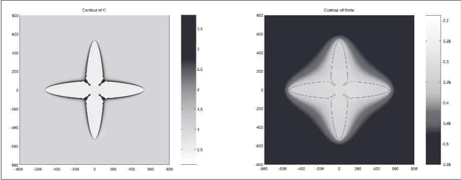
the diffusion fields can be seen in Figure 1, where a typical

concentration (c / c_∞) and temperature field (θ) of a

simula-tion with Lewis number 40 is shown on the left and right respectively.

Where the concentration field, on the left-hand side, forms a very steep interface, the temperature field varies more gradually (the contour of the interface is plotted in the Figure to show where the interface lies). Typically, this complexity has led modellers to rely primarily on relatively simple numerical methods; however in this work we aim to

Proceedings of the 5th Decennial International Conference on Solidification Processing, Sheffield, July 2007

demonstrate that it is possible, and indeed advantageous, to make use of advanced numerical methods, such as adaptivity, implicit schemes and multigrid. The model is described in the next section before the proposed discretisation method is described and some results are shown. A detailed descrip-tion of the discretisadescrip-tion method, as well as a comparison to widely used explicit methods, can be found in [1].

2. Phase-Field model

The phase-field model used here is the coupled thermal-solute model for the simulation of microstructure formation in dilute binary alloys, given in [2]. The microstructure is

represented by the phase variable φ which divides the liquid

and the solid phases by a diffuse interface. The solid and

liquid phases correspond to φ= 1 and φ= – 1 respectively,

and in the interface region φ varies smoothly between the

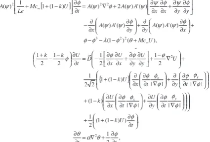
bulk values. The governing equations, in dimensionless form for vanishing kinetic effects, are

[ ] { } , 2 1 , ) ) 1 ( 1 ( 2 1 | | | | ) 1 ( | | | | ) 1 ( 1 2 2 1 2 1 2 1 ~ 2 1 2 1 ), ( ) 1 ( ) (' ) ( ) (' ) ( ) (' ) ( 2 ) ( ) 1 ( 1 1 ) ( 2 ~ 2 2 2 3 2 2 2 t t t U k t y U t x U k t y t x U k U y U y x U x D t U k k U Mc x A A y y A A x y y x x A A A t U k Mc Le A y x y x ∂ ∂ + ∇ = ∂ ∂       ∂ ∂ − + +             ∇ ∂ ∂ ∂ ∂ +     ∇ ∂ ∂ ∂ ∂ − +             ∇ ∂ ∂ ∂∂ +     ∇ ∂ ∂ ∂∂ − + +     ∇ − +       ∂ ∂ ∂ ∂ + ∂ ∂ ∂ ∂ − = ∂ ∂       + ₋ − + − − − +       ∂ ∂ ∂ ∂ +     ∂ ∂ ∂ ∂ −       ∂ ∂ ∂ ∂ + ∂ ∂ ∂ ∂ + ∇ = ∂ ∂     _{+ + −} ∞ ∞ φ θ α θ φ φ φ φ φ φ φ φ φ φ φ φ φ φ φ φ φ θ φ λ φ φ φ ψ ψ φ ψ ψ φ ψ φ ψ ψ ψ φ ψ φ ψ

where ψ= arctan(φy / φx) is the angle between the normal

to the interface and the x-axis, A(ψ) = 1 + ε cos(ηψ) is an

anisotropy function with anisotropy strength ε and mode

number η. The dimensionless coupling parameter is given

as λ= ~D / a2= (a1W0) / d0 with d0 as the chemical capillary

length. Also, a1 = 5√2 / 8 and a2 = 0.6267 [5] to simulate

kinetic free growth with the dimensional solute diffusivity ~

D=Dτ0 / W02, where τo= (d02 / D)a2λ3 / a12is a relaxation time

and W0=d0λ / a1 is a measure of the interface width. The

dimensionless concentration field U is given as

, 1 ) 1 ( 1 / 2 k k k c c U −     − − + = ∞ φ

where c_∞ is the value of the concentration c far from the

interface and k is the partition coefficient. The system

parameters are set to k= 0.15, W0=τ0= 1, ε= 0.02 and

η= 4.0.

The highly nonlinear nature of these time-dependent PDEs is clearly apparent due to the anisotropy terms in the phase equation and the solute trapping term in the concentration equation, respectively. A further numerical difficulty arises from the fact that the ratio of diffusivities

(Lewis number) Le=α / D is typically ~ 103_{. Here, the Lewis}

number is set to 40 in order to compare the simulation results with results published in [3].

3. Numerical methods

Due to the nature of the phase-field method, where the variables may change only in a small region relative to the computational domain, adaptive mesh refinement is a natural choice and leads to a computationally efficient method. The governing equations are discretised with a finite difference approximation based upon a quadrilateral, uniform, refined mesh. The adapted meshes are non-uniform in the sense that we allow hanging nodes.

3.1 Spatial discretisation

For all of the computational results presented in this paper, second order finite difference schemes have been used. Important for the stability of the numerical method is the fact that the interface is always in the refined region. To ensure this, adaptive refinement is used based upon an elementwise gradient criterion. The final adaptive refined mesh for the simulation shown in Figure 1 is shown in Figure 2.

The mesh shows a very high resolution in the interface region in order to resolve the steep gradient of the phase and concentration field. Also, refinement away from the interface on coarser mesh levels is used to represent the temperature field accurately.

but that this increases rapidly over time and converges to a constant value which depends upon the choice of the tolerance. The final step size of the BDF2 method is slightly more than 0.18 which is 60 times bigger than the reported maximum time step size of 0.003, for the explicit Euler method on the same mesh size, in [3].

3.4 Non-linear multigrid solver

When using implicit time discretisation methods it is neces-sary to solve a system of non-linear algebraic equations at each time step. A multigrid solver for adaptive refined meshes has been developed based upon the Full Approximation Scheme (FAS) for resolving the non-linearity and the adaptive multigrid approach, see [4]. A major property of

the multigrid method is the h-independent convergence,

which means that the convergence rate does not depend on the spatial element size. This has been demonstrated for the isothermal case, where we showed that our method

converged almost independently of h with the same rate for

uniform as well as adaptively refined meshes, see [1].

4. Results

The dendritic growth simulation is undertaken with the model parameters given in section 2. The only free

para-meter to choose is the coupling parapara-meter λ, which depends

3.2. Time discretisation

A widely used choice for temporal discretisation of phase-field models are explicit methods such as the forward Euler scheme, see [3]. As already mentioned, the explicit methods suffer from a time step restriction. This condition is neces-sary in order to ensure the stability of the discretisation scheme, and, for some non-linear systems, this can lead to

excessively small time steps (Δt). In order to overcome this

restriction the use of implicit time integration methods is proposed in this paper. These methods may be designed to be unconditionally stable, which means that the time step size does not depend on the space step size in order to ensure stability. Use of a second-order Backward Difference Formula (BDF2), combined with the described spatial discretisation, leads to a second-order time and space method. This is not true for second-order explicit time integration methods, such as Runge-Kutta or the trapezoidal or midpoint rules because the stability of these methods are also only preserved by the same condition as for the forward Euler scheme.

It is very clear that the BDF2 method converges with significantly larger time steps than the explicit Euler method

and can provide comparable accuracy with much larger Δt,

see [1].

3.3 Variable step size control

The initial conditions typically considered for this problem consist of a small region of solid at the centre of the domain, known as the nucleus. The growth velocity of the initial nucleus is very high at the beginning of the simulation, before the interface becomes unstable and dendritic arms begin to grow, ultimately reaching a steady-state velocity. Consequently, adaption of the time steps for the BDF2 method is likely to be efficient and leads to an adaptive time and space discretisation method. The adaptive time stepping algorithm we use is based on the following rule: if the local time discretisation error is less or equal to the

tolerance Tol, this time step is accepted and the next time

step size is increased, whereas, if the local error is bigger

than Tol, the step is rejected and redone with a smaller time

step. Figure 3 illustrates the progression of the time step size

for tα / d02= 0…260000, for the tolerance Tol= 0.00125 on

a mesh with minimum spacing of h / W0= 0.78. One can see

that a very small time step size is used right at the beginning

iterations

Time step

Variable time stepping

Tol=0.00125

Figure 3: The evolution of the time step size for a given tolerance.

iterations

Curvature of the tip

Radius of curvature

Le=40, lambda=2, Mo=0.07, R0=10d0

iterations Tip velocity

Le=40, lambda=2, Mo=0.07, R0=10d0

Ve

locity

Proceedings of the 5th Decennial International Conference on Solidification Processing, Sheffield, July 2007

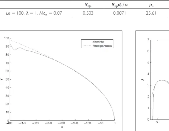
Note, however, that the actual tip radius is only of limited usefulness when comparing simulation results against theoretical predictions. Instead, a calculated optimal para-bolic tip radius is typically used, especially since theories which are based on the Ivantsov solution assume that the dendritic arm takes a parabolic shape. This parabolic tip radius is calculated by using a least squares fit. Therefore, it is assumed that a parabola which is lying on the x-axis and pointing to the growth direction can be represented as [5] y2_{= – 2.0ρ(x – x}

0) by introducing a Cartesian

coor-dinate system (x,y) which is situated at the tip position x0.

After extracting the right dendritic arm from the contour

plot (φ= 0), and shifting to the origin of the new

coordi-nate system, the least-squares fit produces the unknown

parameter ρ and x0. The least-squares fit and the actual

arm of the dendrite are shown in Figure 5. The accuracy of the unknown parameters depend on the choice of the fitting interval, and in our case the interval is chosen to be ~

x= [– 50…– 5]. When extending or varying the interval, the

calculated tip radius lies between 11.95 and 12.23, which

gives the same average value as obtained when using ~x.

Additionally, the Péclet number Pe=Vtipρ / 2α can

now be calculated. All the parameters shown in Table 1 are in very good agreement with the published results in [3].

4.2 Gibbs-Thomson comparison

The dimensionless form of the anisotropic Gibbs-Thomson relation for evaluation along the x-axis is given as [3]

Ui= (– d0(1 – 15ε) / ρa – θi) / Mc∞ where ρa is the actual tip

on the choice of the solutal diffusivity coefficient D. This

parameter is set to D= 2a2 here, whereby it follows that

λ= 2 and the capillarity length d0= 0.441942. In order to

simulate a pure four-fold symmetry, the radius of the initial

seed is taken as R0≈ 10d0 or R0≈ 78d0. The rectangular

domain is chosen to be Ω= [– 800,800]2 _{with Dirichlet}

boundary conditions (φ= – 1, U= 0, θ= – 0.55). A typical

result for the simulation of the model described in section 2 is shown in Figure 1 where the Lewis number is 40 which leads to a significant difference in the length scales. Figure 1

shows the mixture concentration c / c_∞ and the

dimension-less temperature field θ on the left-hand side and the

right-hand side respectively where the initial seed radius is set to

r0≈ 10d0. The contour φ= 0 is also plotted into the right

picture to show where the interface lies.

4.1 Parameter study

Two ways of verifying our results will be discussed in this section. Firstly, the simulation results will be compared against the results published in [3] and secondly a compar-ison to the anisotropic Gibbs-Thomson relation will be performed.

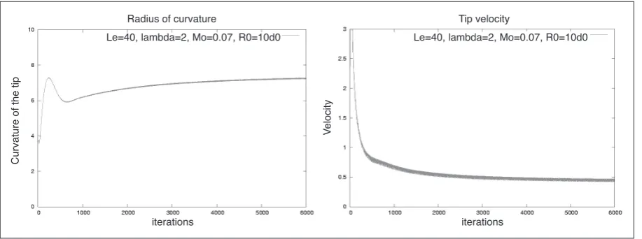
Figure 4 shows the actual tip radius of curvature ρa

and the tip velocity Vtip developing over time measured

along the x-axis for t= 0…1000 on a mesh with minimum

step size h / W0= 0.78. Both parameters indicate that the

simulation has reached a steady-state. The steady-state values are shown in Table 1 for two different initial solute concentrations.

Table 1: Steady-state simulation parameters for Le= 40 and different initial solute concentration.

Vtip Vtipd0 / α ρa ρ ρ / d0 Vtipρ / (2α)

Le = 40, λ = 2, Mc_∞ = 0.07 0.452 0.0040 7.22 12.10 27.38 0.0546

Le = 40, λ = 2, Mc_∞ = 0.01 0.793 0.0070 13.40 22.05 49.89 0.1744

Table 2: Steady-state simulation parameters for Le= 100.

Vtip Vtipd0 / α ρa ρ ρ / d0 Vtipρ / (2α)

Le = 100, λ = 1, Mc_∞ = 0.07 0.503 0.0071 25.61 47.63 53.89 0.1913

Figure 5: Comparison of the original dendrite arm with the fitted parabola.

radius of curvature and θi is the interface temperature, which

can both be obtained directly from the simulation results at each time step. The exact position, in the interface region, where the interface temperature should be evaluated is discussed in [2] and [3]. For comparisons with this relation, the interface concentration is calculated at each time step

by computing the value of U directly behind the interface

where φ≈ 1, see [3]. The simulation was undertaken with

an initial seed radius of R0≈ 78d0 which led to the same

steady-state parameters as [3], see Table 1. As one can see in Figure 6, a very good agreement can be demonstrated for the comparison with the theoretical Gibbs-Thomson prediction.

4.3 The effect of increasing Lewis number

Further increases in the Lewis number lead to a signifi-cant increase in the tip velocity, which can be a source of numerical instability. When using an explicit time integra-tion scheme, this would cause the time steps size to drop. With our proposed implicit method, where the time step is additionally adapted, the final time step size can be kept relatively constant.

Results for the case with Le= 100 are also presented

in [3], which show a good agreement with our results in Table 2, apart from a slight difference in the Péclet number that may be due to the fact that we obtain our results on a finer mesh than the authors in [3], which should lead numerically to higher accuracy.

5. Conclusions

This paper presents an efficient fully adaptive numerical scheme for the simulation of dendritic alloy growth in an undercooled melt in two dimensions. In order to solve efficiently on meshes with a very fine spatial resolution, adaptive meshing and a second-order implicit time discreti-sation method are used and coupled with variable time step size control. This combination allows much larger time steps which reduces the execution time drastically compared to explicit time integration methods since there is no artificial stability restriction imposed on the time step size.

The presented steady-state simulation results show very good agreement with published results and theoretical prediction by the Gibbs-Thomson relation. Further studies may be undertaken, including the application of this numer-ical method to problems with very high Lewis number and realistic material parameters.

References

1. J. Rosam, P.K. Jimack, and A.M. Mullis, Report 2006.4, School of Computing Research report series, University of Leeds, UK, 2006, submitted to Journal of Computational Physics (http:// www.comp.leeds.ac.uk/research/pubs/reports/2006/2006_ 04.pdf).

2. J.C. Ramirez, C. Beckermann, A. Karma, and H.-J. Diepers, Phys. Rev. E, 69 (2004) p. 051607.

3. J.C. Ramirez, and C. Beckermann, Acta Mater., 53 (2005), 1721–1736.

4. U. Trottenberg, C. Oosterlee, and A. Schüller, Multigrid, Academic Press, 2001.