Cooperative Learning and its Application to
Emotion Recognition from Speech
Zixing Zhang, Eduardo Coutinho, Jun Deng, and Bj¨orn Schuller,
Member, IEEE
Abstract
In this article we propose a novel method for highly efficient exploitation of unlabeled data – Cooperative Learning. Our
approach consists of combining Active Learning and Semi-Supervised Learning techniques, with the aim of reducing the costly
effects of human annotation. The core underlying idea of Cooperative Learning is to share the labeling work between human and
machine efficiently in such a way that instances predicted with insufficient confidence value are subject to human labeling, and
those with high confidence values are machine labeled. We conducted various test runs on two emotion recognition tasks with a
variable number of initial supervised training instances and two different feature sets. The results show that Cooperative Learning
consistently outperforms individual Active and Semi-Supervised Learning techniques in all test cases. In particular, we show that
our method based on the combination of Active Learning and Co-Training leads to the same performance of a model trained on
the whole training set, but using 75% fewer labeled instances. Therefore, our method efficiently and robustly reduces the need for
human annotations.
Index Terms
Cooperative learning, active learning, semi-supervised learning, multi-view learning, supervised learning, emotion recognition,
acoustics.
I. INTRODUCTION
Although in the past few years great advances have been made in the field of emotion recognition from speech [1]–[3], a
central challenge remains to be the size and nature of the training corpora used in the development of such pattern recognition
systems. Indeed, the training corpus often needs to comprise a sufficient amount of data that allows for a good generalization
performance to the task at hand (including a good sample of the types of acoustic signals characteristic of a particular application).
Unfortunately, the scarcity of labeled data seriously compromises the development of many recognition systems, which in
turn limits their performance in practical scenarios [4]–[6]. As an example, popular emotional speech databases such as the
Berlin Emotional Speech Database (EMO-DB) and eNTERFACE include around one hour of recordings each [7], [8], whereas
available corpora for automatic speech recognition comprise hundreds of hours of labeled data. It stands to reason, nevertheless,
Zixing Zhang, Eduardo Coutinho, and Jun Deng are with the Machine Intelligence & Signal Processing Group, Institute for Human-Machine Communication, Technische Universit¨at M¨unchen (Germany). E-mail:{zixing.zhang, e.coutinho, jun.deng}@tum.de
Eduardo Coutinho is also with the School of Music, University of Liverpool (United Kingdom).
that in comparison with the small amount of available labeled data, there is a wide range of unlabeled data ideally suited for
the development of speech emotion recognition systems. Such (unlabeled) data are nowadays pervasive in digital format and are
relatively easy and inexpensive to collect (e. g., from online sources). Therefore, the exploitation of these large amounts of data
to enhance (emotion) recognition systems’ performance is increasingly attracting attention from a wider range of researchers
[9]–[11].
In the last few years, several approaches have been proposed to deal with unlabeled data, one of the most promising being
Active Learning(AL) [12]. AL aims at achieving greater accuracy with fewer training labels by (actively) choosing the data
from which it learns. AL algorithms select from large pools of unlabeled data those instances that are the ‘most informative’
for the task being modeled, and subsequently query a human or machine annotator for labeling. There are various strategies
by which the informativeness of unlabeled samples can be processed (usually referred to as query strategies). One of the
simplest strategies is to allow the model (or active learner) to determine the uncertainty of the predictions on unlabeled data
based on a previously trained model (uncertainty sampling AL), and then query an annotator for the labeling of those with the
least certain classification [13]. Another common strategy is the so-called query-by-committee, whereby the predictions for
unlabeled data are obtained from multiple models (previously) trained on the same data (typically models represent competing
hypotheses to solve the same task). In this type of strategy the data considered to be the most informative are those with the
lowest agreement across classifiers [14]. Other AL query strategies include the expected-error-reduction method, which aims
to measure how much its generalization error is likely to be reduced [15]; the expected-model-change-based method, which
chooses those instances that have a greater impact on the current model [16]; and the diversity-density-related method, which
aims to maximize the learning benefits of relevance feedback on retrieving documents [17].
It has been shown that AL strategies can greatly reduce the time-consuming and expensive human labeling work and still
achieve good performance levels [12]. Nonetheless, AL approaches still require a considerable amount of human annotation. A
possible solution that allows one to overcome this expensive limitation is to useSemi-Supervised Learning (SSL) techniques,
which also aim at using unlabeled data in an efficient way but without the intervention of human annotators. In this context,
various combinations of AL and SSL methods have been proposed and can be found in some pattern recognition literature (see
for instance [18], [19], and [20]). A popular approach is to combine AL with Self-Training.Self-Trainingis an SSL technique
that permits automatically annotating unlabeled data by using a preexisting model trained on a small amount of labeled data.
Typically, the most confident predictions for unlabeled points (and their predicted labels) are added to the training set, and the
classifier is re-trained with the new (larger) set. This procedure is then repeated iteratively until a certain performance target is
achieved. Because it does not require the intervention of human annotators, this approach is attractive and a useful option to
enhance the robustness of existing classifiers [21], [22]. Due to this advantage, Self-Trainingis a convenient option to tandem
with AL to reduce the amount of human labeling, as it has been demonstrated, for instance, in spoken language understanding
[19] and handwritten digit and text classification [20].
Another SSL method with the potential to mitigate the limitations of AL is multi-view learning (MVL; [22]–[24]). MVL
focuses on improving the learning performance by training different models concurrently and optimizing them by exploiting
proposed in the literature. It focuses on training two learners by maximizing the mutual agreement on two distinct “views”
of the unlabeled data set. The algorithm relies on three assumptions or conditions: (a) sufficiency: each “view” is sufficient
for classification on its own, (b)compatibility: the target functions in both “views” predict the same labels for co-occurring
features with high probability, and (c) conditional independence: the “views” are conditionally independent given the class
label [25]. Initially, two separate classifiers are trained on the same (labeled) data using the features from each “view.” Then,
the most confident predictions of each learner on the unlabeled data are used to train each other (i. e., are added to the training
set iteratively). Essentially, each classifier is trained with its own data plus the additional training examples provided by the
other classifier. MVL techniques in general are less restrictive than Co-Training in particular and can be applied with two or
more “views” on the data and with less restrictive conditions in terms of conditional independence. MVL schemes have been
applied in several areas, such as biometrics [26], intelligent transportation [27], and handwriting [28] classification. In emotion
recognition from acoustic signals, they have also been successfully applied with relevant improvements over Self-Training[29],
[30].
In this article, we propose a new method for combining AL and SSL techniques to improve a preexistent acoustic emotion
recognition system. To do so, we implement various learning algorithms for retraining a classifier consisting of Support Vector
Machines (SVMs) [31]. We first implement and compare the use of Supervised Learning (SL) [22] variants for improving
the performance of a preexisting classifier. In particular, we focus on Passive Learning (PL) [12], AL and a novel method
that we call ‘Co-active Learning’ (hereaftercoAL). coAL is inspired by the concept of MVL, and it consists of implementing
two different “views” into AL. This strategy diverges from Co-Testing [23] by allowing both “views” to select the data to
be annotated independently, rather than finding the ‘contention points’. At this stage, we also introduce a new type of AL
query strategy based on dynamic medium certainty [32] as an alternative to the traditional least certainty sampling strategy. Our
second step is to implement Self- and Co-Training SSL learning methods to improve the same classifier. Finally, our third
step is to tandem various combinations of AL and SSL approaches (hereinafter referred to as ‘Cooperative Learning’ (CL))
with the aim of improving the classifier performance and reducing the amount of human annotation through machine labeling.
The CL approaches proposed here involve selecting unlabeled instances with medium confidence values and subjecting them
to human annotation (AL phase), and afterwards to select those instances with high confidence values and subject them to
machine annotation (SSL phase). In summary, three CL strategies are proposed: (a) single-view Cooperative Learning (svCL),
which combines AL and Self-Training; (b) mixed-view Cooperative Learning (xvCL), a combination of AL and Co-Training,
and (c) multi-view cooperative learning (mvCL), which explores the use of coAL and Co-Training.
The remainder of this article is structured as follows. In Section II, we make a short introduction to SVMs and their prediction
‘confidence values’. Then, we describe the various learning strategies and methods used in this paper, including SL (Subsection
III-A), SSL (Subsection III-B), and CL (Subsection III-C). Next, we introduce the databases (Section IV) and feature sets
(Section V) used in this paper in, and show the experimental setups and results (including a comparison between CL and
other approaches) in Section VI. Finally, in Section VII we discuss our findings, present our conclusions and suggest possible
II. SVMS ANDCONFIDENCE
In order to investigate CL based on confidence values and exemplify its application to acoustic emotion recognition, we
decided on SVMs as the classification method. The rationale is that SVMs have a mature theoretical foundation [33], and were
officially employed by the INTERSPEECH 2009 (IS09) Emotion Challenge (EC) [34] and its offshoots.
SVMs are supervised learning models based on the concept of decision hyperplanes that define decision boundaries, i. e.,
planes that separate sets of objects having different class memberships. SVMs perform classification tasks by constructing a set
of hyperplanes in a multidimensional space that separates cases of different class labels. The goal of SVMs is to maximize the
separation between classes, which consists of finding the hyperplane that has the largest distance to the nearest training data
point of any class (also known as functional margin), since the larger the margin, the lower the generalization error of the
classification task. In practice, training instances belonging to two or more categories are used to determine the hyperplane that
best discriminates amongst different classes (that with the widest possible gap). The testing instances are then mapped onto this
multi-dimensional space and the side of the gap they fall on determines the predicted categories.
Formally, given a set of examples[xi, yi], i= 1,2, . . . , m, wherexi ∈Rd is ad-dimensional feature vector, andyi∈ {0,1}
is a corresponding prediction of each example, the maximum margin separating hyperplane can be found by solving the
following optimization problem:
maxαW(α) = m
X
i=1
αi−1
2 m
X
i,j=1
y(i)y(j)αiαjK(xi, xj)
subject to:0≤αi≤T, i= 1, . . . , m
m
X
i=1
αiy(i)= 0,
(1)
where theα0isthat are Lagrangian multipliers satisfy the above constraints, T is a defined constant, andK(xi, xj)is a kernel
function that can be linear, polynomial, radial basis, or sigmoidal. To classify a given test example, the following function is
implemented:
f(x) = m
X
i
αiyiK(xi, x) +b, (2)
whereb is the ‘bias’ term that is often assumed to have zero mean. The sign of this function determines the category of the
test example.
The output value of SVMs is the distance of a specific point from the separating hyperplane. To convert these distances to
probability estimates within the range of [0,1]there are various approaches (including parametric and nonparametric methods).
In the experiments described in this article, we employed a parametric method of logistic regression proposed in [35], which is
one of the most frequently used approaches to transform the output distances of SVMs into (pseudo) probabilistic values [36].
This method assumes that the posterior probability consists of finding the parametersA andB for a form of sigmoid function:
P(y|f(x)) = 1
1 +exp(Af(x) +B), (3)
classes is equal to 1. In the special case of binary recognition tasks the decision threshold is 0.5. Therefore, the ‘winning’ class
is determined when the posterior probability is higher than 0.5. The confidence value for the predicted class can be obtained by
the equation:
C(x) =||P0(x)−P1(x)|| (4)
whereP0(x), P1(x)are the posterior probabilities for classes ‘0’ and ‘1’, respectively.
III. METHODOLOGY
In this section we describe the various algorithms used to retrain a SVM for improving the classification performance based
on exploitation of unlabeled data. For all the algorithms described, we assume the following premises: (1) A small set of
labeled dataL exists, where – as above –L= ([x1, y1], . . . ,[xl, yl]),xi is ad-dimensional feature vector xi∈Rd, andyi is
the label for each set of data; (2) a large set of unlabeled dataU is available, where U = (x01, . . . , x0u), and ul and x0j is a
d-dimensional feature vector; and (3) at each iteration, a subset of ninstances is selected fromN for labeling (either by a
human or a machine annotator).
A. Human annotator: PL, AL, and coAL
Fig. 1 shows the pseudocode description of PL, AL (least and medium certainty query strategies) and coAL algorithms.
Algorithm 1describes a standard PL algorithm, whereby unlabeled instances are randomly selected from a pool of samples
and subject to human annotation, before being added to the training set. Algorithm 2 describes a traditional AL approach
based on the least certainty query strategy. This algorithm starts by classifying all instances of the unlabeled data pool U using
the model previously trained on the labeled data L. Then, the confidence values assigned to each instance are ranked and
stored in a queueQ(in descending order). Finally, a subsetNa ofU corresponding to those instances predicted with lowest
confidence values is subject to human annotation. This sequential process is repeated until a predefined number of instances are
selected (which depends on the size of the databases).Algorithm 3also describes the traditional AL algorithm, but with a novel
query strategy based on the selection of those instances predicted with medium certainty levels for further annotation. The
rationale for adopting a medium certainty query strategy is the potential advantage of avoiding the selection of noisy data,
which can be caused by unreliable annotations [37] or distortions of the (acoustic) pattern [38] as demonstrated in [39]. This is
particularly important for acoustic emotion recognition owing to the comparably high degree of ambiguity. This approach has
been previously used in [32].
The new query strategy diverges from Algorithm 2 in which the instances that are closest to the middle of the queue Q
are the ones selected for human annotation (unlike the ones with lowest confidence values, as it is characteristic of the least
Algorithm 1: Passive Learning (PL)
Repeat:
1) Randomly select subsetNp from unlabeled setU
2) Ask human experts to label the selected subset Np
3) RemoveNp from the unlabeled setU,U =UrNp
4) Add Np to the labeled set L,L=L ∪ Np
Algorithm 2: Active Learning (AL) with least certainty query strategy
Repeat:
1) (Optional) Upsample the training setL to obtain even class distributionLD
2) UseL/LD to train a classifier H, and then classify the unlabeled setU
3) Rank the data based on the prediction confidence values C and store them in queueQ
4) Select a subset Na whose elements are in thebottomof the ranking queueQ(least certainty)
5) Submit the selected subset Na to human annotation
6) RemoveNa from the unlabeled setU,U =UrNa
7) Add Na to the labeled set L,L=L ∪ Na
Algorithm 3: Active Learning (AL) with medium certainty query strategy
Repeat:
1) (Optional) Upsample the training setL to obtain even class distributionLD
2) UseL/LD to train a classifier H, and then classify the unlabeled setU
3) Rank the data based on the prediction confidence values C and store them in queueQ
4) Select subsetNa whose elements are in themiddleof the ranking queueQ(medium certainty)
5) Submit the selected subset Na to human annotation
6) RemoveNa from the unlabeled setU,U =UrNa
7) Add Na to the labeled set L,L=L ∪ Na
Algorithm 4: Co-Active Learning (coAL)
Given (addition): A learning domain with featuresV
Repeat:
1) Split the domain featuresV into two “views”:V1,V2, andV1∩V2=∅ 2) Foriin 1, 2
a) (Optional) Upsample each “view” to even class distributionVDi
b) UseVi/VDi to train classifierHi, and classify U, respectively.
c) Rank the data based on the prediction confidence valuesC and store them in queueQ
d) Select a subset Na whose elements are in the middle of the ranking queue Q(medium certainty)
3) Submit the selected subsetsNca=Na1∪ Na2 to human annotation 4) RemoveNcafrom the unlabeled setU,U =UrNca
5) Add Nca to the labeled setL,L=L ∪ Nca
Fig. 1. Pseudocode description of the four types of supervised learning used in this article: Passive Learning (Algorithm 1), Active Learning based on theleast certainty query strategy (Algorithm 2) and on themediumcertainty query strategy (Algorithm 3), and co-Active Learning (Algorithm 4).
the unlabeled data pool. Formally, the query function is defined as:
Query(x) =
1, if CD(x) = arg min x
|C(x)−Cm|,
0, otherwise,
(5)
whereC(x)represents the prediction confidence value for a given instancex, and Cm is the confidence value of the instance
located in the center of the ranking queue. Ideally, for uniformly distributed predictions, Cmwould be 0.5. Nonetheless, in
practice this value is not fixed. Instead, it varies due to the changes on the unlabeled data pool as learning progresses (instances
moved to the training set).
Finally,Algorithm 4extends the idea of MVL to AL and uses a medium certainty query strategy. Here, the feature domainV
Then, each “view” is used to create a classifier H, and each classifier is tested on the unlabeled data poolU. The unlabeled
instances predicted by each model with medium confidence values are then delivered to a human annotator for labeling. After
that, these instances are added (together with the new label) to the training set and removed from the unlabeled data pool.
There are three possibilities regarding the selection of a particular instance by the two “views”: 1) if an instance is not selected
by any of the two “views”, it will be discarded in this iteration; 2) if an instance is selected by any of the two “views”, that
instance plus the given label will be added to the training set once; 3) if an instance is selected by both “views”, it will be
added twice to the training set together with the common class label (because it was annotated by a human). The whole process
is repeated until a predetermined number of iterations of the learning process is achieved.
B. Machine annotator: Self-Training and Co-Training
Fig. 2 shows the pseudocode describing the two types of SSL algorithms considered in this paper: Self-Training (Algorithm
5) and Co-Training (Algorithm 6). Self-Training is based on the principle of highest certainty or agreement, in such a way that
the predicted classes with higher certainty levels are automatically labeled and added to the training set. Similarly to AL, the
query function for Self-Training is as follows:
Query(x) =
1, ifCD(x) = arg min x
|C(x)−1|,
0, otherwise.
(6)
In comparison with Self-Training, Co-Training uses two models trained and tested on two different “views” of the data. In
each iteration of the algorithm, the two “views” select the instances independently. Therefore, in one iteration, an instance is
either discarded (low certainty predictions), added once (high certainty predictions by one of the two classifiers), added twice
with the same label (high certainty and similar predictions by the two classifiers), or added twice with different labels (high
certainty but different predictions by the two classifiers).
C. Cooperative annotator
As mentioned in the introduction, AL algorithms generally improve a model’s performance, but they still require a considerable
amount of human intervention. SSL techniques, instead, exploit machine labeling of data, yet usually cannot improve the
performance of an existing classifier as much as AL techniques can when the same number of instances are labeled [23]. In order
to take advantage of the best of both approaches we propose a CL algorithm that combines AL and SSL that allows sharing
the labeling effort between human and machine annotators while attempting to mitigate the limitations of both algorithms. In
SSL, the absence of sufficient instances for a particular category in the initial training set can lead to poor performance for that
category. This is because the instances with higher confidence estimates selected by the SSL algorithm are generally inclined to
those categories with more samples and correct classification. This problem often leads to a cycle in which the dominating
categories are recognized increasingly better, and the opposite happens with the less represented categories. This drawback is
absent in AL, which mostly ignores the dominating categories. Therefore, the combination of two learning approaches may
Algorithm 5: Self-Training
Repeat:
1) (Optional) Upsample training set Lto even class distributionLD
2) UseL/LD to train classifierH, then classifyU
3) Select a subset Nst that contains those instances predicted with the highest confidence values
4) RemoveNst from the unlabeled setU,U =UrNst
5) Add Nst to the labeled set L,L=L ∪ Nst
Algorithm 6: Co-Training
Given (addition): A learning domain with featuresV
Repeat:
1) Divide the domain featuresV into two “views”:V1, V2, andV1∩V2=∅ 2) Foriin 1, 2
a) (Optional) Upsample each “view” of data to even class distributionVDi
b) UseVi/VDi to train classifierHi, and then classify U.
c) Select a subsetNsi that contains those instances predicted with the highest confidence values
3) RemoveNct=Ns1∪ Ns2 from the unlabeled setU,U =UrNct
4) Add Nct=Ns1∪ Ns2 to the labeled setL,L=L ∪ Nct
Fig. 2. Pseudocode description of the two types of SSL used in this paper: Self-TrainingAlgorithm 5and Co-TrainingAlgorithm 6.
added to the training set. Even though only the instances with the highest confidence values are chosen, some of these instances
can be misclassified. As in the previous case, this noise is accumulated and increasingly affects the performance of the classifier.
Once again, AL can compensate for this limitation. We will execute AL in each iteration before implementing SSL, re-train the
classifier with newly (manually) labeled instances, and re-classify the unselected instances with the new model for SSL.
In this article, we propose three particular combinations of AL and SSL algorithms (see Fig. 3). First, we implemented
AL followed by Self-Training, which we refer to as svCL (see Algorithm 7). Second, we combined AL and Co-Training,
hereinafter xvCL (see Algorithm 8). Third, we consider coAL followed by Co-Training (mvCL) (see Algorithm 9). Fig. 3
describes the details of the algorithms pertaining to these three CL strategies. For all experiments described, the learning cycle
was stopped when a predefined number of instances are selected (see Table III). Also, in order to deal with the potential
problem of imbalanced class distributions, we employed data upsampling by random subsampling in all algorithms in order to
add more instances belonging to the less represented classes to the training set.
IV. DATABASES
In order to evaluate the application of CL to emotion recognition from speech and demonstrate its robustness across corpora,
we chose the FAU Aibo Emotion Corpus (FAU AEC) and the Speech Under Simulated and Actual Stress (SUSAS) database.
Both databases consist of natural speech samples, and are widely used in the field of speech emotion recognition [7], [34], [40],
[41].
A. FAU Aibo Emotion Corpus
The FAU AEC [42] (the official corpus of the IS09 EC [34]) contains audio recordings of German-speaking children
Algorithm 7: single-view Cooperative Learning (svCL)
Repeat:
1) Execute AL based on an initial training set L, and obtain a subsetNa for human labeling (cf. Algorithm 3)
2) RemoveNa from the unlabeled setU (U0=UrNa), and addNa it to the labeled data setL (L0=L ∪ Na)
3) Execute Self-Training based on a training set L0, and obtain a subsetN
st for machine labeling (cf.Algorithm 5)
4) RemoveNst from the unlabeled setU0 (U =U0rNst), and add Nst it to the labeled setL0 (L=L0∪ Nst)
Algorithm 8: mixed-view Cooperative Learning (xvCL)
Given (addition): A learning domain with featuresV
Repeat:
1) Execute AL based on initial training setL, and obtain a subsetNa for human labeling (cf. Algorithm 3)
2) RemoveNa from the unlabeled setU (U0=UrNa), and addNa to the labeled setL (L0 =L ∪ Na)
3) Execute Co-Training based on training set L0, and obtain a subsetN
ct for machine labeling (cf.Algorithm 6)
4) RemoveNctfrom the unlabeled setU0 (U =U0rNct), and addNct it to the labeled data setL0 (L=L0∪ Nct)
Algorithm 9: multi-view Cooperative Learning (mvCL)
Given (addition): A learning domain with featuresV
Repeat:
1) Execute coAL based on an initial training set L, and obtain a subsetNca (cf. Algorithm 4)
2) RemoveNcafrom the unlabeled setU (U0 =U rNca), and add Nca it to the labeled setL (L0=L ∪ Nca)
3) Execute Co-Training based on a training setL0, and obtain a subsetN
ct for machine labeling (ref. Algorithm 6)
4) RemoveNctfrom the unlabeled setU0 (U =U0rNct), and addNct it to the labeled setL0 (L=L0∪ Nct)
Fig. 3. Pseudocode description of the three types of Cooperative Learning proposed: single-view Cooperative Learning (svCL), mixed-view Cooperative Learning (xvCL), and multi-view Cooperative Learning (mvCL).
responding to their commands by producing a series of fixed and predetermined behaviors. Nevertheless, the Aibo robot did
sometimes disobey the children’s commands, which provoked various types of emotional reactions.
The recordings include speech samples from 51 children (30 females) with ages ranging from 10 to 13 years that were taken
at two different German schools to which we will refer to in this paper as MONT and OHM. The whole corpus comprises a
total of 9.2 hours of speech without pauses, which was recorded through a DAT-recorder (16 bit, 48 kHz down-sampled to
16 kHz) placed on a wireless headset. The recordings were segmented into turns using a pause threshold of 1 s. Five students of
advanced linguistics were then asked to listen to the various samples and to annotate each one of them by selecting one specific
label (from a set of 11 predefined labels) to describe the emotional character of the sample. The labels used were: neutral,
angry,touchy,reprimanding,emphatic,surprise,joyful,helpless,motherese,bored, andothers. If more than three annotators
assigned a specific label to a speech sample (majority voting), that label was chosen to describe the emotional character of the
segment.
In our experiments we use the same natural speech corpus used in the IS09 EC [34] that consists of 18 216 instances
taken from the full database. Each instance consists of a manually defined chunk of speech longer than a word and shorter
than a ‘turn’, which is defined based on syntactic-prosodic criteria. The original 11 classes were mapped onto two cover
classes: one consisting of NEGative emotion labels (angry,touchy,reprimanding,emphatic), and the others consisting of all
non-negative states (IDL; for more information about the database development and data processing please refer to [34]). In
order to guarantee speaker independence, we used the data recorded at the OHM school as the unlabeled data pool (9 959), and
B. Speech Under Simulated and Actual Stress Database
The SUSAS database contains audio recordings of speakers in various (actual and simulated) stress conditions and organized
in different domains. To the purpose of this article we focus on the “Actual Speech Under Stress” domain, which includes
audio recordings of speech produced in the “Scream Machine” scenario, one of the subject motion-fear tasks. In this scenario,
7 speakers (3 female) were taken in a roller-coaster (the “Scream Machine”) ride for about 90 s and asked to repeat words from
a 35-word vocabulary card (held in their hands) at different moments. Each speaker performed the task twice.
In the task scenario, different levels of stress were spontaneously evoked by the dynamics of the roller-coaster ride, resulting
in the various levels of stress being expressed in the voice. A total of 1 642 utterances were collected during the rides (sampled
at 8 kHz, 16 bit). Subsequently these utterances were segmented into words, resulting in 3 593 instances that were then annotated
for stress levels (i.e., neutral, medium, high stress, and screaming) based on the time and position during the ride. Similarly
to the FAU AEC database, in our experiments we converted the four stress classes of SUSAS into two stress-intensity cover
classes – HIGH (i.e.,high stress and screaming) andLOW (i.e.,neutral and medium stress). So as to perform a speaker
independent evaluation, we chose 1 064 instances recorded from one male speaker and one female speaker as the validation set,
and used the remaining instances (2 529) for the unlabeled pool set. The details of the SUSAS database instances used in this
article are shown in Table I (for more information please refer to [43]).
TABLE I
DISTRIBUTION OF SPEAKERS AND INSTANCES PER PARTITION OF THEFAU AIBOEMOTIONCORPUS(AEC) [42]AND THESPEECHUNDERSIMULATED ANDACTUALSTRESS(SUSAS) [43]. M:MALE; F:FEMALE; NEG:NEGATIVE EMOTIONS; IDL:NEUTRAL AND POSITIVE EMOTIONS; HIGH:HIGH STRESS;
LOW:LOW STRESS.
# speakers # instances per class
FAU AEC M F NEG IDL Σ
Pool 13 13 3 358 6 601 9 959
Validation 8 17 2 465 5 792 8 257
Σ 21 30 5 823 12 393 18 216
SUSAS M F HIGH LOW Σ
Pool 3 2 1 116 1 413 2 529
Validation 1 1 500 564 1 064
Σ 4 3 1 616 1 977 3 593
V. ACOUSTICFEATURES
In order to evaluate the robustness of the methods proposed in this paper to different feature sets, we selected two standard
sets of acoustic features used in the INTERSPEECH 2009 Emotion Challenge (EC) [34] and the INTERSPEECH 2010 (IS10)
Affect Sub-Challenge (ASC) [44]. Both feature sets were created for affect-related pattern recognition tasks (including emotional
states). All features were extracted using the openSMILE framework [45].
A. The INTERSPEECH 2009 Emotion Challenge Feature Set
The IS09 EC feature set contains 384 features that result from a systematic combination of 16 Low-Level Descriptors (LLDs)
square (RMS) frame energy, pitch frequency (normalized to 500 Hz), harmonics-to-noise ratio (HNR) by autocorrelation function,
and mel-frequency cepstral coefficients (MFCC) 1–12 (in full accordance to HTK-based computation). The 12 functionals used
are mean, standard deviation, kurtosis, skewness, minimum, maximum, relative position, range, and offset and slope of linear
regression of segment contours, as well as its two regression coefficients with their mean square error (MSE) applied on a
chunk. The complete feature set contains 16×2×12 = 384attributes per chunk (or instance). Table II presents the details of
the complete feature set.
TABLE II
THEIS09 ECAND THEIS10 ASC ACOUSTIC FEATURE SETS USED IN OUR EXPERIMENTS:LOW-LEVEL DESCRIPTORS(LLDS)AND RESPECTIVE FUNCTIONALS. THE∗SYMBOL INDICATES THE FEATURES BELONGING TO VIEW-1FOR THECO-TRAINING AND CO-ACTIVELEARNING(COAL)
ALGORITHMS.
LLD(∆) Functionals
IS09 EC feature set (384)
ZCR mean
RMS Energy standard deviation energy
F0 kurtosis, skewness
HNR extremes: value, rel. position, range
MFCC 1-12∗ linear regression: offset, slope, MSE
IS10 ASC feature set (1 582)
PCM loudness position maximum/minimum
MFCC 0-14∗ algorithmic mean, standard deviation log Mel freq. band 0-7 skewness, kurtosis
line spectral pairs freq. 0-7 linear regression coefficients 1/2
F0 linear regression error quadratic/absolute
F0 envelope quartile 1/2/3
voicing probability quartile range 2-1/3-2/3-1 jitter local percentile 1/99
jitter consec. frame pairs percentile range 99-1 shimmer local up-level 75/90
B. The INTERSPEECH 2010 Affect Sub-Challenge Feature Set
The IS10 ASC feature set is an extension of the IS09 EC feature set designed to cover a wider range of features relevant
for paralinguistic information retrieval [44]. The IS10 ASC feature set consists of 1 582 acoustic features and transliteration
(including those capturing non-linguistic characteristics) obtained by systematic ‘brute-force’ feature (over)generation in three
phases: 1) extraction of 38 LLDs and smoothing by simple moving average low-pass filtering; 2) computing the first order
regression coefficients on features extracted in 1) (full HTK compliance); 3) apply 21 functionals to 1) and 2). After that,
we discarded 16 features because their values were always zero (e.g., minimum F0). Furthermore, we added 2 new features:
number of discernible pitches and number of discernible pitches per second. Table II shows the LLDs, regression coefficients
and functionals for the IS10 AEC feature set. For more details see [44].
VI. EXPERIMENTS ANDRESULTS
In this section, we evaluate the performance of CL (and compare it to the various learning strategies described in Section III)
A. Experimental Setup
As described in Section II, we use SVMs as the modeling paradigm for evaluating the various machine learning algorithms.
In accordance with the IS09 EC baseline specifications, the SVMs were initially trained with a Sequential Minimal Optimization
(SMO) algorithm with a linear kernel and a complexity constant of 0.05. Logistic regression modeling was enabled to allow
converting the SVMs’ output distances to confidence values. In terms of performance evaluation, we use the unweighted average
recall (UAR) index as the primary performance measure (following the recommendation in [34]). As mentioned in Section III,
an upsampling strategy was adopted for even class distribution (i.e., one time more for the ‘NEG’ instances for the FAU
AEC). The training process was repeated 20 times with different initializations of the random generator for each experimental
condition.
We conducted four different experiments to evaluate the performance and robustness of our newly proposed CL methods.
The first two experiments were designed to evaluate the performance of the various learning methods with different numbers of
initial training instances using the FAU AEC corpus and the IS09 EC feature set. In this paper we use 200 and 500 instances
of the FAU AEC database for initial training, which corresponds to approximately 2 % and 5 %, respectively, of the whole
pool. In the third experiment, we evaluate the various learning strategies with the FAU AEC corpus and a new feature set
(IS10 ASC) so as to establish the robustness of CL for different feature sets (using 200 initial training instances). In the final
experiment, we use a new corpus (SUSAS) with the IS10 ASC feature set to evaluate the robustness of CL across tasks (with
100 initial training instances, approximately 5 % of the whole pool). For the four experiments, the UARs obtained after the
initialsupervised training were: 1) 60.9 % (std = 1.8); 2) 62.6 % (std = 1.1); 3) 64.4 % (std = 1.3); and 4) 58.6 % (std = 2.5).
The performances when training the SVMs with thefull set of training data were: 1) 67.7 %; 2) 67.7 %; 3) 67.2 %; and 4)
64.6 % (UARs).
TABLE III
PREDEFINED NUMBER OF SELECTED INSTANCES FOR SEMI-SUPERVISED(SSL),ACTIVE(AL),AND COOPERATIVE LEARNING(CL).H/M:HUMAN/MACHINE LABELING
# SSL AL CL
H M H M H M
Aibo 0 5 000 5 000 0 2 400 6 000
SUSAS 0 1 250 1 250 0 600 1 500
In all experiments, the instances not used for the initial training were used for the unlabeled data pool. Given that more
unlabeled data are necessary for machine-supervised learning than for human-supervised learning, at each learning iteration, we
select 200 instances for labeling for AL and coAL algorithms, and 500 instances for Self-Training and Co-Training. For the
MVL-based algorithms (coAL and Co-Training), each “view” chooses an equal number of instances, that is, in each iteration
each “view” selects, respectively, 100 and 250 instances. Given the smaller size of the SUSAS database (approximately 25 % of
the FAU AEC) used in experiment four, fewer instances are selected in each learning iteration: 50 (AL and coAL) and 125
(Self-Training and Co-Training).
For the creation of each “view” used for multi-view learning, we split the full feature set into two partitions - one comprising
order to be balanced between the two “views”), and the fact that MFCCs are, on their own, a common set of features used in
speaker identification and speech recognition that increasingly found its way into general paralinguistics. Nonetheless, although
such a feature separation is only related to LLDs and not to higher level features of functionals or linguistics, the features in
the two views may not be conditionally independent, as for example, a change in the signal which affects F0 or energy, etc.,
will also affect the MFCCs. However, the effect will be different, thus likely adding complementary information. Furthermore,
the experimental results in [46] demonstrate that such feature separation criterion applied to multi-view learning is valid and
effective. The ratio of attributes (view-1/view-2) is 288/96 for the IS09 EC feature set, and is 630/952 for the IS10 ASC feature
set.
B. Self-Training and Co-Training
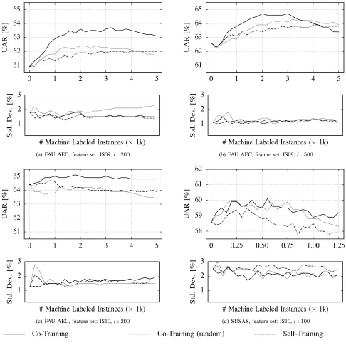
In Fig. 4, we show the average and standard deviation of the UAR measure for the Self-Training and Co-Training approaches
under study. The error measures shown correspond to the average of the individual performances across 20 independent runs of
the learning process for all four experiments described in this paper.
The first observation is that Co-Training using the feature separation based on cepstral LLDs improves the initial classification
performance in all our four experimental scenarios. Co-Training using random feature separation did not lead to improvements
using the IS10 feature set and the FAU AEC database (see Fig. 4 (c)). Self-Training led to improvements in the experiments
using the IS09 feature set, but not in those using the IS10 one (see Figs. 4 (c) and (d)). Overall, Co-Training with cepstral LLDs
feature separation seems to be more robust than the other two approaches when using different numbers of initial supervised
training instances, different databases and different feature sets. Furthermore, it outperforms the other approaches after only
a few iterations, which suggests that this algorithm leads to a faster learning process and better generalization performance.
Finally, it is also evident that the performance of Co-Training degrades after a certain number of learning iterations. Previous
work (e.g., [25], [47]) has demonstrated that this phenomenon can be attributable to the exchange of mislabeled instances
between the different “views.”
C. PL, AL and coAL
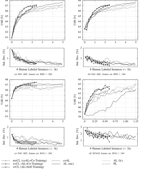
In this section we evaluate the performance of the PL, AL with least (lc) and medium (mc) certainty query strategies, and
coAL algorithms. Fig. 5 shows the performance figures averaged across 20 independent runs of the whole training process (and
respective standard deviations) for the four experimental scenarios (the results of CL, also shown, will be described later).
As can be seen, the sequential addition of the human-labeled instances to the training set (200 per iteration for FAU AEC
and 50 for SUSAS) led to improvements in the performance of the classifier for all four supervised learning approaches.
Nonetheless, contrary to our expectations, the coAL approach did not show an improvement over the AL algorithms. The
AL approach with the medium certainty query strategy, especially in relation to the FAU AEC database, delivers the best
global performance. The exception to this rule, as it can be seen on Fig. 5 (d), is the performance for the SUSAS database,
which is particularly worse than the other algorithms for fewer human labeled instances. In this task, the AL with the least
61
62
63
64
65
0
1
2
3
4
5
U AR [%]
61
62
63
64
65
0
1
2
3
4
5
U AR [%]
1
2
3
Std. De v . [%]# Machine Labeled Instances (
×
1k)
(a) FAU AEC, feature set: IS09,l: 200
1
2
3
Std. De v . [%]# Machine Labeled Instances (
×
1k)
(b) FAU AEC, feature set: IS09,l: 500
61
62
63
64
65
0
1
2
3
4
5
U AR [%]
58
59
60
61
62
0
0.25
0.50
0.75
1.00
1.25
U AR [%]
1
2
3
Std. De v . [%]# Machine Labeled Instances (
×
1k)
(c) FAU AEC, feature set: IS10,l: 200
1
2
3
Std. De v . [%]# Machine Labeled Instances (
×
1k)
(d) SUSAS, feature set: IS10,l: 100
[image:14.612.61.547.65.550.2]Co-Training Co-Training (random) Self-Training
Fig. 4. Comparison between Co-Training using the feature separation method based on cepstral LLDs, Co-Training using a random feature separation method, and Self-Training. The charts show the average UARs across 20 independent runs (and respective standard deviations) vs. number ofmachinelabeled instances for the four experiments described in this paper: a) FAU AEC database with the IS09 EC feature set and 200 initial supervised training instances; b) FAU AEC database with the IS09 EC feature set and 500 initial supervised training instances; c) FAU AEC database with the IS10 ASC feature and 200 initial supervised training instances; and d) the SUSAS database with the IS10 ASC feature set and 100 initial training instances.
medium certainty strategy achieve a similar performance to that of the baselines when the models are trained with the full set
of training data. Nevertheless, it uses, respectively, 55 %, 50 %, 70 %, and 65 % fewer human labeled instances in each of the
61 62 63 64 65 66 67 68
0 1 2 3 4 5
U AR [%] 61 62 63 64 65 66 67 68
0 1 2 3 4 5
U AR [%] 1 2 Std. De v . [%]
# Human Labeled Instances (× 1k)
(a) FAU AEC, feature set: IS09,l: 200
1 2 Std. De v . [%]
# Human Labeled Instances (× 1k)
(b) FAU AEC, feature set: IS09,l: 500
61 62 63 64 65 66 67 68
0 1 2 3 4 5
U AR [%] 58 59 60 61 62 63 64 65 66
0 0.25 0.50 0.75 1.00 1.25
U AR [%] 1 2 Std. De v . [%]
# Human Labeled Instances (× 1k)
(c) FAU AEC, feature set: IS10,l: 200
1 2 3 Std. De v . [%]
# Human Labeled Instances (× 1k)
(d) SUSAS, feature set: IS10,l: 100
[image:15.612.61.555.65.658.2]mvCL (coAL+Co-Training) xvCL (AL+Co-Training) svCL (AL+Self-Training) coAL AL (mc) AL (lc) PL
TABLE IV
MEANS AND STANDARD DEVIATIONS OFUARPERFORMANCE MEASURE OBTAINED BY AVERAGING THE RESULTS BETWEEN ITERATIONS4AND12 (800∼2 400INSTANCES FORFAU AEC,AND200∼600INSTANCES FORSUSAS). VALUES ARE SHOWN FORPASSIVELEARNING(PL), ACTIVE LEARNING(AL),CO-ACTIVELEARNING(COAL),AND SINGLE-/MIXED-/MULTI-VIEWCOOPERATIVELEARNING(SVCL/XVCL/MVCL)FOR THE FOUR
EXPERIMENTAL CONDITIONS.
Avg. (a) (b) (c) (d)
UAR FAU AEC FAU AEC FAU AEC SUSAS
[%] IS09,l:200 IS09,l:500 IS10,l:200 IS10,l:100
[image:16.612.157.451.301.541.2]PL 65.7±0.8 66.8±0.6 65.6±0.7 62.4±2.0 AL 66.1±0.6 67.0±0.5 66.0±0.8 63.2±1.7 coAL 65.9±0.6 66.4±0.9 65.7±0.7 62.3±1.8 svCL 66.4±0.7 66.9±0.6 66.1±0.8 63.9±1.5 xvCL 66.7±0.5 67.2±0.4 66.7±0.8 63.9±1.7 mvCL 66.7±0.5 67.2±0.5 66.6±0.8 63.1±1.9
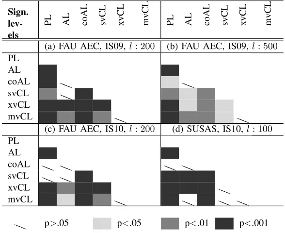
TABLE V
SIGNIFICANCE LEVELS OBTAINED FROM THE STATISTICAL COMPARISON(STUDENT’St-TEST)OF THEUARPERFORMANCE MEASURES BETWEEN ITERATIONS4AND12 (800∼2 400INSTANCES FORFAU AEC,AND200∼600INSTANCES FORSUSAS). VALUES ARE SHOWN FORPASSIVELEARNING (PL), ACTIVELEARNING(AL),CO-ACTIVELEARNING(COAL),AND SINGLE-/MIXED-/MULTI-VIEWCOOPERATIVELEARNING(SVCL/XVCL/MVCL)FOR
THE FOUR EXPERIMENTAL CONDITIONS.
Sign. lev-els
PL AL coAL svCL xvCL mvCL PL AL coAL svCL xvCL mvCL
(a) FAU AEC, IS09,l: 200 (b) FAU AEC, IS09,l: 500
PL AL coAL
aa aa
svCL
aa
xvCL mvCL
aa aa
(c) FAU AEC, IS10,l: 200 (d) SUSAS, IS10,l: 100
PL AL coAL
aa aa aa aa
svCL
aa aa
xvCL
aa
mvCL
aa aa aa aa
aa p>.05 p<.05 p<.01 p<.001
D. Cooperative Learning
We now turn to our final set of algorithms that combine AL and SSL techniques. As mentioned earlier, we focus on three
particular methods: svCL, xvCL, and mvCL. In these approaches only a maximum of 2 400 and 600 human labeled instances
could be considered for the FAU AEC and the SUSAS databases, respectively. This is due to the fact that both AL and SSL
algorithms independently select instances from the unlabeled pool for human and machine (respectively) labeling at each
learning iteration. Therefore, the comparisons with the previous models are only made for a maximum of 12 iterations of
the learning algorithm (when the maximum number of human labeled instances is achieved). Given the inconclusive results
obtained in the previous section regarding the query strategy, the AL algorithms used in the CL approaches make use of the
with the SUSAS database.
As depicted in Fig. 5, the three CL methods perform globally better than all other algorithms for different numbers of
initial training instances, databases and feature sets. The improvement is evident in all experiments just after a few iterations
of the learning algorithms, the only exception being the experiment with the FAU AEC and the IS10 feature set where the
improvement is clearer at the end of the learning process. Moreover, the standard deviation of UAR exhibits a descending trend,
which indicates that increasingly adding more human labeling instances to the training set makes the system more stable. In
relation to the global performance improvement and human effort minimization, the best UARs obtained with CL algorithms in
the four experimental scenarios (67.2 %, 67.2 %, 67.6 %, 64.9 %) are very close to the baseline performance of the models
trained on the whole pool of labeled data (67.7 %, 67.7 %, 67.2 %, 64.6 %). Nevertheless, CL uses about 75 % fewer labeled
instances in all scenarios and is, therefore, less expensive.
In order to analyze in more detail the performance of the various algorithms, we calculated the average UAR across iterations
4 and 12 (see Table IV) and computed Student’st-tests to statistically compare the performances of the various algorithms (see
Table V). An analysis of both tables confirms our previous observations and clearly indicates that all three CL approaches
(single-, mixed-, and multi-view) generally lead to significantly better performance than all other methods. This is particularly
evident for xvCL (AL and Co-Training), the algorithm that led to the best performance in all four experiments by consistently
and robustly outperforming the other methods. This is consistent with the best performance of Co-Training over Self-Training
as described in Subsection VI-B.
VII. CONCLUSIONS ANDFUTUREWORK
In this article, our main aim was to exploit large amounts of unlabeled (speech) data to enhance the performance of existing
(emotion) classifiers while minimizing the costly work of human labeling. To do so, we tested the use of Supervised Learning
and Semi-Supervised Learning techniques, and we proposed a novel approach that combines both – Cooperative Learning. In
particular we considered three approaches to Cooperative Learning: 1) single-view cooperative learning, which combines Active
Learning and Self-Training; 2) mixed-view Cooperative Learning, which combines Active Learning and Co-Training; and 3)
multi-view Cooperative Learning, which combines co-Active Learning and Co-Training. Furthermore, we evaluated the use of a
medium certainty query strategy for instances selection in Active Learning.
Our experimental results on two well-defined emotion-recognition-from-speech tasks – the FAU Aibo Emotion Corpus and
the Speech Under Simulated and Acted Stress database – show that all three suggested Cooperative Learning algorithms are
superior to all other approaches when using the same number of human-labeled instances for retraining. The results also show
that not only the accuracy of the classifier is improved, but also its stability is enhanced. Furthermore, by varying the amount of
instances used in the initial supervised training phase, using different feature sets, and testing different classification tasks, we
demonstrated that Cooperative Learning is a robust method. In particular, the best performance and robustness were obtained
with the mixed-view Cooperative Learning algorithm, which combines Active Learning and Co-Training. In relation to the type
of query strategy used for instance selection in Active Learning, our results indicate that medium certainty may be a feasible
set sizes and feature sets using the FAU Aibo Emotion Corpus. Nevertheless, the lowest certainty query strategy leads to better
results with the Speech Under Simulated and Acted Stress database and so our results are not conclusive in this respect.
Future extensions of this work should consider larger unlabeled data pools than that considered in our experiments. This
would be important to test further the robustness of Cooperative Learning for very large databases, an ideal scenario for its
application with great relevance for the development of emotion recognition systems for realistic applications. Such data sets
of realistic signals can be created from online sources such as YouTube, recordings of everyday life conversations, among
others. Also, it would be interesting to further demonstrate the robustness of Cooperative Learning with other types of relevant
feature sets (e.g., [48]). In this article we have not explored the use of different query strategies with the aim of improving
robustness within and across tasks. This is an obvious extension of this work and likely candidate methods are sparse instance
tracking and committee-based algorithms. Also, since the methods introduced in this paper were evaluated in the context of
paralinguistic recognition, it would be interesting to evaluate their performance in other classification problems. Finally, it
would be particularly interesting to analyze the effects of various learning strategies proposed in terms of bias-variance trade-off.
This could reveal specific benefits of the various strategies in terms of reducing the various types of errors (bias, variance and
irreducible).
ACKNOWLEDGMENT
The research leading to these results has received funding from the European Research Council in the European Community’s
7th Framework Program under grant agreements No. 338164 (Starting Grant iHEARu), 230331 (Advanced Grant PROPEREMO)
and 289021 (ASC-Inclusion). It was further partially supported by research grants from the China Scholarship Council (CSC)
awarded to Zixing Zhang and Jun Deng. We are very thankful to the editor and three anonymous reviewers for their insightful
comments and relevant suggestions, which helped us to improve the manuscript.
REFERENCES
[1] Y. Attabi and P. Dumouchel, “Anchor models for emotion recognition from speech,”IEEE Transactions on Affective Computing, vol. 4, no. 3, pp. 280–290, 2013.
[2] Y. Kim, H. Lee, and E. Provost, “Deep learning for robust feature generation in audiovisual emotion recognition,” inProc. IEEE International Conference on Acoustics, Speech and Signal Processing (ICASSP), Vancouver, Canada, 2013, pp. 3687–3691.
[3] A. Metallinou, M. Wollmer, A. Katsamanis, F. Eyben, B. Schuller, and S. Narayanan, “Context-sensitive learning for enhanced audiovisual emotion
classification,”IEEE Transactions on Affective Computing, vol. 3, no. 2, pp. 184–198, 2012.
[4] T. Vogt, E. Andr´e, and J. Wagner, “Automatic recognition of emotions from speech: A review of the literature and recommendations for practical
realisation,” inAffect and Emotion in Human-Computer Interaction. Berlin, Germany: Springer, 2008, pp. 75–91.
[5] B. Schuller, A. Batliner, S. Steidl, and D. Seppi, “Recognising realistic emotions and affect in speech: State of the art and lessons learnt from the first
challenge,”Speech Communication, vol. 53, no. 9, pp. 1062–1087, 2011.
[6] Z. Zeng, M. Pantic, G. I. Roisman, and T. S. Huang, “A survey of affect recognition methods: Audio, visual, and spontaneous expressions,”IEEE Transactions on Pattern Analysis and Machine Intelligence, vol. 31, no. 1, pp. 39–58, 2009.
[7] B. Schuller, B. Vlasenko, F. Eyben, M. W¨ollmer, A. Stuhlsatz, A. Wendemuth, and G. Rigoll, “Cross-corpus acoustic emotion recognition: Variances and
strategies,”IEEE Transactions on Affective Computing, vol. 1, no. 2, pp. 119–131, 2010.
[9] L. Devillers, L. Vidrascu, and L. Lamel, “Challenges in real-life emotion annotation and machine learning based detection,”Neural Networks, vol. 18, no. 4, pp. 407–422, 2005.
[10] B. Schuller, “The computational paralinguistics challenge,”IEEE Signal Processing Magazine, vol. 29, no. 4, pp. 97–101, 2012.
[11] B. Schuller and A. Batliner,Computational Paralinguistics: Emotion, Affect and Personality in Speech and Language Processing. New York, NY: John Wiley & Sons, 2013.
[12] B. Settles, “Active learning literature survey,” Department of Computer Sciences, University of Wisconsin–Madison, Wisconsin, WI, Tech. Rep., 2009.
[13] J. Zhu, H. Wang, B. K. Tsou, and M. Ma, “Active learning with sampling by uncertainty and density for data annotations,”IEEE Transactions on Audio, Speech, and Language Processing, vol. 18, no. 6, pp. 1323–1331, 2010.
[14] R. Liere and P. Tadepalli, “Active learning with committees for text categorization,” inProc. 14th National Conference on Artificial Intelligence and 9th Innovative Applications of Artificial Intelligence Conference (AAAI/IAAI), Providence, RI, 1997, pp. 591–596.
[15] N. Roy and A. McCallum, “Toward optimal active learning through sampling estimation of error reduction,” inProc. 24th Annual International Conference on Machine Learning (ICML), Williamstown, MA, 2001, pp. 441–448.
[16] B. Settles and M. Craven, “An analysis of active learning strategies for sequence labeling tasks,” inProc. Empirical Methods in Natural Language Processing (EMNLP), Honolulu, HY, 2008, pp. 1070–1079.
[17] Z. Xu, R. Akella, and Y. Zhang, “Incorporating diversity and density in active learning for relevance feedback,” inProc. 29th European Conference on Information Retrieval (ECIR), Rome, Italy, 2007, pp. 246–257.
[18] A. McCallum and K. Nigam, “Employing EM in pool-based active learning for text classification,” inProc. 15th Annual International Conference on Machine Learning (ICML), Madison, WI, 1998, pp. 359–367.
[19] G. Tur, D. Hakkani-T¨ur, and R. E. Schapire, “Combining active and semi-supervised learning for spoken language understanding,”Speech Communication, vol. 45, no. 2, pp. 171–186, 2005.
[20] X. Zhu, J. Lafferty, and Z. Ghahramani, “Combining active learning and semi-supervised learning using gaussian fields and harmonic functions,” inProc. 20th Annual International Conference on Machine Learning (ICML) Workshop on The Continuum from Labelled to Unlabelled Data, Washington DC, 2003, pp. 58–65.
[21] O. Chapelle, B. Sch¨olkopf, A. Zienet al.,Semi-Supervised Learning. Cambridge, MA: MIT Press, 2006.
[22] X. Zhu, “Semi-supervised learning literature survey,” Department of Computer Sciences, University of Wisconsin at Madison, Madison, WI, Tech. Rep. TR 1530, 2006.
[23] I. Muslea, S. Minton, and C. Knoblock, “Active + semi-supervised learning = robust multi-view learning,” inProc. 19th Annual International Conference on Machine Learning (ICML), Sydney, Australia, 2002, pp. 435–442.
[24] X. Cui, J. Huang, and J.-T. Chien, “Multi-view and multi-objective semi-supervised learning for hmm-based automatic speech recognition,”IEEE Transactions on Audio, Speech, and Language Processing, vol. 20, no. 7, pp. 1923–1935, 2012.
[25] A. Blum and T. Mitchell, “Combining labeled and unlabeled data with co-training,” inProc. 11th Annual Conference on Computational Learning Theory (COLT), Madison, WI, 1998, pp. 92–100.
[26] H. Bhatt, S. Bharadwaj, R. Singh, M. Vatsa, A. Noore, and A. Ross, “On co-training online biometric classifiers,” inProc. IEEE International Joint Conference on Biometrics (IJCB), Washington DC, 2011, pp. 1–7.
[27] A. Gepperth, “Co-training of context models for real-time vehicle detection,” inProc. IEEE IV Symposium, Alcala de Henares, Spain, 2012, pp. 814–820. [28] V. Frinken, A. Fischer, H. Bunke, and A. Foornes, “Co-training for handwritten word recognition,” inProc. 11th International Conference on Document
Analysis and Recognition (ICDAR), Beijing, China, 2011, pp. 314–318.
[29] J. Liu, C. Chen, J. Bu, M. You, and J. Tao, “Speech emotion recognition using an enhanced co-training algorithm,” inProc. IEEE International Conference on Multimedia and Expo (ICME), Beijing, China, 2007, pp. 999–1002.
[30] A. Mahdhaoui and M. Chetouani, “Emotional speech classification based on multi view characterization,” inProc. 20th International Conference on Pattern Recognition (ICPR), Istanbul, Turkey, 2010, pp. 4488–4491.
[31] C. Cortes and V. Vapnik, “Support-vector networks,”Machine Learning, vol. 20, no. 3, pp. 273–297, 1995.
[32] Z. Zhang and B. Schuller, “Active learning by sparse instance tracking and classifier confidence in acoustic emotion recognition,” inProc. Interspeech, Portland, OR, 2012, no pagination.
[33] V. Vapnik,The Nature of Statistical Learning Theory, 2nd ed. Berlin, Germany: Springer, 1999.
[35] J. Platt, “Probabilistic outputs for support vector machines and comparisons to regularized likelihood methods,” inAdvances in large margin classifiers, A. Smola, P. Bartlett, B. Sch¨olkopf, and D. Schuurmans, Eds. Cambridge, MA: MIT Press, 1999, pp. 61–74.
[36] R. Duda, P. Hart, and D. Stork,Pattern Classification, 2nd ed. New York, NY: John Wiley & Sons, 2001.
[37] M. Grimm and K. Kroschel, “Evaluation of natural emotions using self assessment manikins,” inProc. IEEE Workshop on Automatic Speech Recognition and Understanding (ASRU), San Juan, PR, 2005, pp. 381–385.
[38] M. You, C. Chen, J. Bu, J. Liu, and J. Tao, “Emotion recognition from noisy speech,” inProc. IEEE International Conference on Multimedia and Expo (ICME), Toronto, Canada, 2006, pp. 1653–1656.
[39] Z. Zhang, F. Eyben, J. Deng, and B. Schuller, “An agreement and sparseness-based learning instance selection and its application to subjective speech
phenomena,” inProc. 5th International Workshop on Emotion Social Signals, Sentiment & Linked Open Data, satellite of LREC 2014, Reykjavik, Iceland, 2014, pp. 21–26.
[40] A. Hassan, R. Damper, and M. Niranjan, “On acoustic emotion recognition: Compensating for covariate shift,”IEEE Transactions on Audio, Speech, and Language Processing, vol. 21, no. 7, pp. 1458–1468, 2013.
[41] L. Zao, D. Cavalcante, and R. Coelho, “Time-frequency feature and AMS-GMM mask for acoustic emotion classification,”IEEE Signal Processing Letters, vol. 21, no. 5, pp. 620–624, 2014.
[42] S. Steidl,Automatic Classification of Emotion-Related User States in Spontaneous Speech. Berlin, Germany: Logos, 2009.
[43] J. Hansen and S. Bou-Ghazale, “Getting started with SUSAS: A speech under simulated and actual stress database,” inProc. Eurospeech, Rhodes, Greece, 1997, pp. 1743–1746.
[44] B. Schuller, S. Steidl, A. Batliner, F. Burkhardt, L. Devillers, C. M¨uller, and S. Narayanan, “The INTERSPEECH 2010 paralinguistic challenge,” inProc. Interspeech, Makuhari, Japan, 2010, pp. 2794–2797.
[45] F. Eyben, M. W¨ollmer, and B. Schuller, “openSMILE – the Munich versatile and fast open-source audio feature extractor,” inProc. 18th ACM International Conference on Multimedia (MM), Florence, Italy, 2010, pp. 1459–1462.
[46] Z. Zhang, J. Deng, and B. Schuller, “Co-training succeeds in computational paralinguistics,” inProc. IEEE International Conference on Acoustics, Speech and Signal Processing (ICASSP), Vancouver, Canada, 2013, pp. 8505–8509.
[47] X. Zhu and A. B. Goldberg, “Introduction to semi-supervised learning,”Synthesis lectures on artificial intelligence and machine learning, vol. 3, no. 1, pp. 1–130, 2009.
[48] S. Ntalampiras and N. Fakotakis, “Modeling the temporal evolution of acoustic parameters for speech emotion recognition,”IEEE Transactions on Affective Computing, vol. 3, no. 1, pp. 116–125, 2012.
Zixing Zhangreceived his master degree (2010) in physical electronics from Beijing University of Posts and Telecommunications, China. He is currently pursuing his Ph. D. degree as a Researcher in the Machine Intelligence & Signal Processing (MISP) Group at
the Institute for Human-Machine Communication at Technische Universit¨at M¨unchen (TUM) in Germany. He authored and co-authored more than twenty publications in peer-reviewed journals and conference proceedings. His current research focuses on efficient machine
learning algorithms for acoustic emotion recognition and automatic speech recognition.
Eduardo Coutinhoreceived his diploma in Electrical Engineering and Computer Sciences from the University of Porto (Portugal, 2003), and his doctoral degree in Affective and Computer Sciences from the University of Plymouth (UK, 2009). Currently, Coutinho
is a postdoctoral fellow at the Technische Universit¨at M¨unchen, an Affiliate Researcher at the Swiss Center for Affective Sciences (CISA), and an Honorary Research Fellow at the School of Music from the University of Liverpool. His research interests include Neural Networks, Affective Computing, and Music Perception and Cognition. Dr. Coutinho is a member of the INNS, ISRE and
Jun Dengreceived his bachelor degree (2009) in electronic and information engineering from Harbin Engineering University and his
master degree (2011) in information and communication engineering from Harbin Institute of Technology (HIT), Heilongjiang/China. He is currently pursuing his Ph. D. degree in the MISP Group at TUM. His interests are machine learning methods such as transfer
learning with an application preference to emotion recognition in speech.
Bj¨orn Schullerreceived his diploma in 1999, his doctoral degree for his study on Automatic Speech and Emotion Recognition in 2006, and his habilitation and Adjunct Teaching Professorship in the subject area of Signal Processing and Machine Intelligence
in 2012, all in electrical engineering and information technology from TUM. He is a tenured Full Professor heading the Chair of Complex Systems Engineering at the University of Passau/Germany and a Senior Lecturer in Machine Learning in the Department
of Computing at the Imperial College London in London/UK. Dr. Schuller is president of the Association for the Advancement of Affective Computing (AAAC), elected member of the IEEE Speech and Language Processing Technical Committee, and member