White Rose Research Online URL for this paper:
http://eprints.whiterose.ac.uk/5005/
Monograph:
Vickers, D., Rees, P. and Birkin, M. (2003) A New Classification Of UK Local Authorities
Using 2001 Census Key Statistics. Working Paper. School of Geography , University of
Leeds.
School of Geography Working Paper 03/03
Reuse
See Attached
Takedown
If you consider content in White Rose Research Online to be in breach of UK law, please notify us by
WORKING PAPER
03/03
A NEW CLASSIFICATION OF UK LOCAL AUTHORITIES
USING 2001 CENSUS KEY STATISTICS
Daniel Vickers, Phil Rees, Mark Birkin
School of Geography
University of Leeds
Leeds LS2 9JT
United Kingdom
E- mail:
[email protected]
[email protected]
[email protected]
ABSTRACT
The 2001 Census has been successfully administered and the Census Organisations are
currently engaged in processing the returns. A very large and rich dataset will be produced
for the 58,789,194 people of the UK. The Census Area Statistics, for example, delivers 190
tables containing about 6 thousand unique counts relating to the characteristics of the UK
population, for output areas and all higher geographies. This paper represents the first results
of a project that aims to develop, in collaboration with the Office for National Statistics, a set
of general purpose classifications at different geographic scales, including households,
neighbourhoods, wards, local authorities and to link the classifications at different levels
together. The paper reports on the methods used and results of a classification of the UK’s
434 Local Authorities, using the Key Statistics released in February 2003. This initial
classification and description of methods will feed into the ONS/GROS/NISRA project to
classify Local Authorities for the whole UK.
Further data or digital versions of the classification system are available on request from
ACKNOWLEDGEMENTS
The authors wish to thank firstly the ESRC and the ONS who provided funding for this
project in the form of a CASE PhD studentship for Daniel Vickers. Many thanks must go to,
Richard Webber, Tony Champion, John Stillwell, Graham Clarke, Danny Dorling, John
Charlton, Alison Whitworth and Samantha Poole who have shown help and support and
CONTENTS
Page
Abstract
ii
Acknowledgements
iii
Contents
iv
List of Figures
vi
List of Tables
vi
1
Introduction
1
2
A Review of the general procedures used in classification
2
2.1
What attributes?
2
2.2
How many clusters?
3
2.3
Which method of clustering?
5
2.3.1 The procedure used in k-means classifications
5
2.3.2 The advantages of arranging a classification hierarchically
7
3
A Review of previous classifications of local authorities
8
4
The Aims of the Paper
10
5
The process of classification
10
5.1
Variable selection
10
5.2
Clustering the Local Authorities
19
6
Classification Outputs
24
6.1
The Structure of Families, Group and Classes
24
6.2
LA to cluster look-up table
27
6.3
Pen Portraits
31
6.3.1
Family A: Urban UK
32
6.3.1.1
Group A1 : Indus trial Legacy
33
6.3.1.1.1 Class A1a: Industrial Legacy
33
6.3.1.2
Group A2 : Established Urban Centres
34
6.3.1.2.1 Class A2a: Struggling Urban manufacturing
35
6.3.1.2.2 Class A2b: Regional Centres
36
6.3.1.2.3 Class A2c: Multicultural England
37
6.3.1.2.4 Class A2d: M8 Corridor
38
6.3.1.3
Group A3 : Young and Vibrant Cities
39
6.3.1.3.1 Class A3a: Redeveloping Urban Centres
40
6.3.1.3.2 Class A3b: Young Multicultural
41
6.3.2
Family B: Rural UK
42
6.3.2.1
Group B1 : Rural Britain
43
6.3.2.1.1 Class B1a: Rural Extremes
44
6.3.2.1.2 Class B1b: Agricultural Fringe
45
6.3.2.1.3 Class B1c: Rural Fringe
46
6.3.2.2
Group B2 : Coastal Britain
47
6.3.2.2.1 ClassB2a: Coastal Resorts
48
6.3.2.2.3 Class B2c: Aged Coastal Resorts
50
6.3.2.3
Group B3 : Averageville
51
6.3.2.3.1 Class B3a: Mixed Urban
52
6.3.2.3.2 Class B3b: Typical Towns
53
6.3.2.4
Group B4 : Isles of Scilly
54
6.3.2.4.1 ClassB4a: Isles of Scilly
54
6.3.3
Family C: Prosperous Britain
55
6.3.3.1
Group C1: Prosperous Urbanites
56
6.3.3.1.1 Class C1a: Historic Cities
57
6.3.3.1.2 Class C1b: Thriving Outer London
58
6.3.3.2
Group C2: Commuter Belt
59
6.3.3.2.1 Class C2a: Commuter Belt
59
6.3.4
Family D: Urban London
60
6.3.4.1
Group D1: Multicultural Outer London
61
6.3.4.1.1 Class D1a: Multicultural Outer London
61
6.3.4.2
Group D2: Mercantile Inner London
62
6.3.4.2.1 Class D2a: Central London
63
6.3.4.2.2 Class D2b: The City of London
64
6.3.4.3
Group D3: Cosmopolitan Inne r London
65
6.3.4.3.1 Class D3a: Afro- Caribbean Ethnic Boroughs
66
6.3.4.3.2 Class D3b: Multicultural Inner London
67
6.3.5
Family E: Northern Irish Heartlands
68
6.3.5.1
Group E1: Northern Irish Heartlands
68
6.3.5.1.1 Class E1a: Northern Irish Urban Growth
69
6.3.5.1.2 Class E1b: Rural Northern Ireland
70
6.4
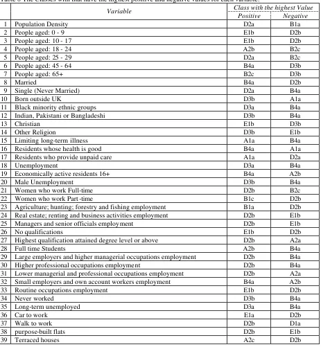
The Clusters with the highest and lowest values
71
6.5
Similarities of the Las
72
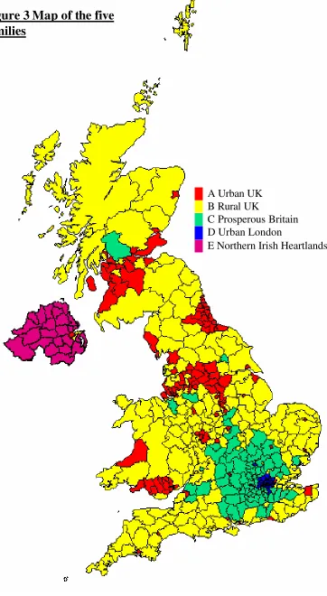
6.5
Mapping out the Clusters
72
References
83
Appendix A List of variables showing inclusion, rejection or merger
84
Appendix B Calculation of the 56 variables from Key Statistics National
Report tables
89
LIST OF FIGURES
Page
1 Correlation matrix of age variables
16
2 The distance between the most dissimilar local authorities within
merged clusters
23
3 Map of the Five Families
73
4 Map of the three groups within the family A Urban UK
74
5 Map of the four groups within the family B Rural UK
75
6 Map of the two groups within the family C Prosperous Britain
76
7 Map of the three groups within the family D Urban London
77
8 Map of the seven classes within family A Urban UK
78
9 Map of the nine classes within family B Rural UK
79
10 Map of the three classes within family C Prosperous Britain
80
11 Map of the five classes within family D Urban London
81
12 Map of the two classes within family E Northern Irish Heartlands
82
LIST OF TABLES
Page
1 The variation in size of the UK’s LAs in terms of population and area
1
2 The 129 variables considered for use in the LA Classification
11
3 First 20 Rows and first 5 columns of the component loadings matrix
15
4 The variables with the highest and lowest standard deviation across all LAs
16
5 The final list of 56 variables to be used in the classification.
18
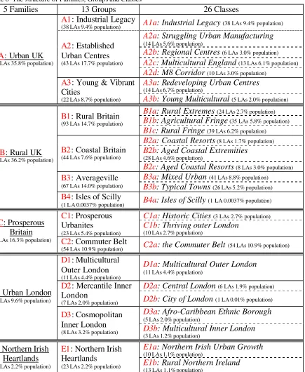
6 The structure of Families, Groups and Classes
26
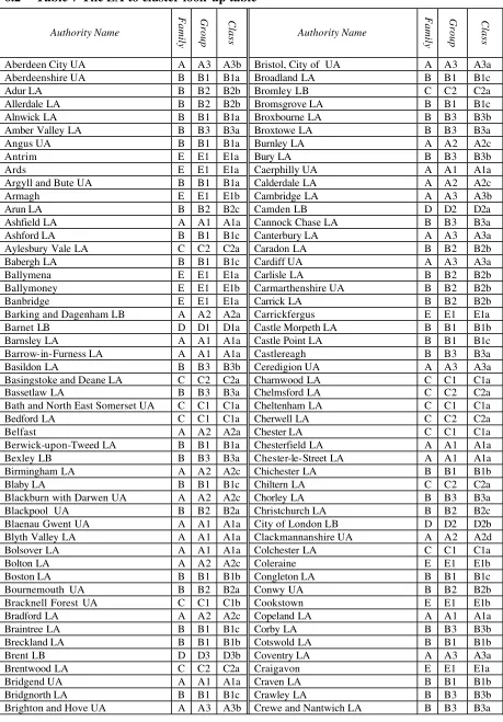
7 The LA to cluster look-up table
27
8 The classes with that have the highest positive and negative values for
1
Introduction
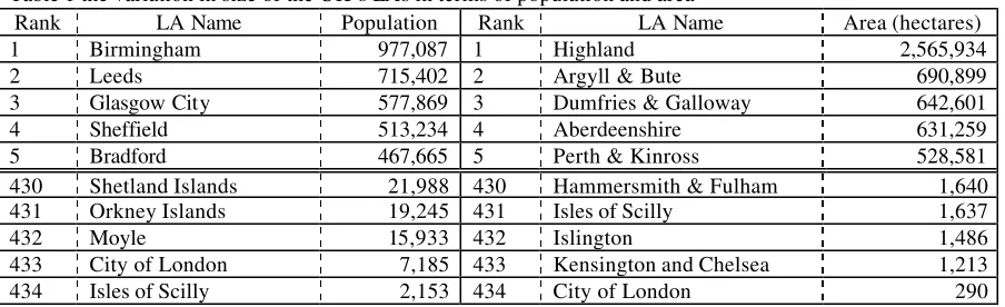
This paper classifies the 434 local authority units that cover the UK into an organised
typology. The UK consists of 434 Local Authorities (LAs); these are a mixture of
Metropolitan Districts, Unitary Authorities, Non-Metropolitan Districts and London
Boroughs in England. Unitary Authorities in Wales, Council Areas in Scotland and District
Council Areas in Northern Ireland. These are the units at which local government operates.
They can vary greatly in size of population and area as shown in table 1. The average size is
[image:8.596.73.525.306.444.2]just over 135,000 people and 56,000 hectares.
Table 1 the variation in size of the UK’s LAs in terms of population and area
Rank
LA Name
Population
Rank
LA Name
Area (hectares)
1
Birmingham
977,087
1
Highland
2,565,934
2
Leeds
715,402
2
Argyll & Bute
690,899
3
Glasgow City
577,869
3
Dumfries & Galloway
642,601
4
Sheffield
513,234
4
Aberdeenshire
631,259
5
Bradford
467,665
5
Perth & Kinross
528,581
430
Shetland Islands
21,988
430
Hammersmith & Fulham
1,640
431
Orkney Islands
19,245
431
Isles of Scilly
1,637
432
Moyle
15,933
432
Islington
1,486
433
City of London
7,185
433
Kensington and Chelsea
1,213
434
Isles of Scilly
2,153
434
City of London
290
Classifications provide a unique way of bringing together areal patterns from a range of
variables, and identify areal similarities and dissimilarities between a range of different
variables (Webber & Craig 1976). The idea of sorting things into categories based on
similarities is not a new one. The basic premise of classification is a primitive one. The nouns
of the English language are little more than labels to describe classes of objects into which
objects can be place. When applied to the animal world objects can be divided into classes
such as pigs, cows, and sheep (Everitt 1993).
In its widest sense, a scheme of classification represents a convenient technique for the
organisation of a large dataset to enhance the efficiency of information recovery. Class labels
describing arrangements of differences and similarities between objects of investigation
provides a convenient summary of the data (Everitt 1993). Put simply classification is the
A classification is a powerful and effective way of condensing a large volume of information,
and summarising it into a single or small number of descriptive variables. Classifications are
especially useful when used on socio-economic data such as that generated from the census.
The census contains large amounts of specific information that in turn can be used as a basis
by which further variables can be derived. It enables the variables that represent the
characteristics of the population within an area to be grouped together using a variety of
statistical techniques. This creates a single value for each area, which is descriptive of both
the area and the people who live there. The classification can be used as a quick and easy
assessment of the properties of an area and it can also be used to compare and contrast that
area with other areas. Classifications enable similar areas, which are geographically spread to
be grouped and by similar reasoning a classification enables areas that are geographically
close or connected to be contrasted. Members of the groups share similarities based on the
characteristics of their residents rather than their geography, the members of the groups do
not have to contiguous.
This paper will start by reviewing the general procedures used in classification, then move on
to review previous classifications of local authority areas. The aims of the paper will then be
set out before presenting the outputs from the classification.
2
Review of the general procedures used in classification
The goal of cla ssification is to arrange N units into M clusters such that the inter-M variation
in attributes is maximise and the intra-M variation in attributes is minimised. However there
are several problems to be solved in developing a classification.
2.1 What attributes?
The way in which the clusters are formed will reflect the variable attributes from which they
are built, the attributes that are selected for the clustering process will drive the classification
and determine whether two objects are put into the same, or a different group. There is no
can be selected based on the factors that are thought to be important and variables are then
simply chosen which, are thought to best represent those factors, in some cases little or no
statistical testing is done on the variable choices. An opposing method would be to use a
series of statistical methods to aid variable choice.
2.2 How many clusters?
The number of cluster selected can significantly alter the result that the classification
produces, by having 11 clusters instead of 10 can completely alter the way in which the
objects are separated. There are no rules as to what is the optimum or best number of cluster
within a classification, each classification needs to be taken on its own merit and previous
decisions such as variable choice and method of clustering will determine the most suitable
number of clusters to be used. There is no standard method for choosing the most suitable
number of clusters but a method that is being increasingly used is by measuring the increase
in distance between the most dissimilar objects within merged clusters as the number of
clusters reduces. The clusters to select are those before a large rise in the distance between
the objects in the same cluster.
Before any further variable selection can be made the variables need to be standardised over
the same range, this ensures that each variable has the same weighting on the classification.
This is important when there is different type of data e.g. population density will give number
of people per an area, however Detached housing is a percentage of all households. If these
variables were clustered without being standardised it would add bias to the dataset. The
method chosen for standardising the variables was to transform them into z-scores. The
method for calculating z-scores is shown in equations 1 & 2, firstly the standard deviation is
calculated. The z-score is then calculated by taking the mean value of the variable away from
the value for that variable for each local authority in turn and then dividing them by the
standard deviation of the variable across all local authorities. This should be repeated for all
The Standard deviation is defined as:
n
x
x
x
i2
)
(
−
=
σ
(1)
The Standard normal variate or z-score is defined as:
x
x
x
Z
ii
σ
−
=
(2)
There are other methods for variable standardisation, for example in the 1999 classification of
Local Authorities the ONS used a range method defined as:
min max
100
x
x
x
Z
ii
−
=
(3)
where
x
maxis the maximum value of
x
and
x
minthe minimum value of
x
For their 2003 Local Authority classification they have decided to change there method
slightly using a 90
th/10
thpercentile method of standardisation, defined as:
10 90
100
x
x
x
Z
ii
=
−
(4)
where
x
90is the 90
thpercentile value of
x
and
x
10is the 10
thpercentile value of
x
,
when the
values of
x
are arranged from lowest to the highest and the cumulative percentage of cases
(LAs).
The standard normal z-score was chosen above other methods as it reduces the effect of
variation within the areas to be classified. By reducing the effect of extreme values on the
classification, the number of very small clusters will be limited, therefore creating a more
usable and valuable classification system.
2.3 Which method of clustering?
The purpose of clustering is to find the best arrangement of N areas into M clusters for any
number M. There are several methods of clustering, the most common and most widely used
is k-means which produces a single predefined solution. In contrast to k-means, hierarchical
clustering procedures produce a series of solutions from which one or more of the most
suitable solutions can be selected.
2.3.1 The procedure used in k-means classifications
The K-means partitions
n
data points with
m
variables into
k
clusters. This results in a
matrix of cluster centres
J
(
k
,
m
)
which minimises the Euclidean sum of squares given by the
equation:
2
1 1
)
(
)
,
(
cjn i
m l
ij
Z
Z
m
k
J
=
∑∑
−
= =
(5)
Where
Z
cj= Value for cluster
cand variable
jij
Variable
1
Variable 2
Step 1:
Select cluster centres, set up
J
(
k
,
m
)
with 2 values
2 12 11 10 9 8 7 6 5 5 3 4 1 2 1
X
X
X
X
X
X
X
X
X
X
X
X
X
X
X
i i i i i i i i i i i i i = = = = = = = = = = = = =Step 2:
Compute distances from objects to clusters
icD
n
i
k
c
1
1
Assign to the cluster with the minimum distance
Step 3:
Compute new average values for cluster centres
c c
i ij
cj
Z
M
Z
∑
/
∈
=
(6)
The previous steps are repeated until a stopping criterion is met, i.e., when there is no further
change in the assignment of the data points
2.3.2 The advantages of arranging a classification hiera rchically
There are two main advantages of using a hierarchical method of clustering
1.
Do not have to predefine the number of clusters
2.
More than one level of classification can be produce which fits into the one above
At the start of the process each object is in a class by itself. Then in small steps the criterion
by which the objects are clustered is relaxed to produces few but larger clusters on the next
step up the hierarchy, this process continues until all the objects being clustered fall within a
single cluster and therefore completing the hierarchy. The process of linking more and more
objects together means that they are amalgamated into larger and larger clusters of increasing
dissimilarity (Ward 1963).
The process of hierarchical clustering is a agglomerative or (bottom- up) approach beginning
with
n
groups each containing 1 object then after merging them together ending with 1 group
Step 1:
Place each object
O
into its own cluster
C
, creating the cluster file
f
therefore:
n n
n
C
C
C
C
C
C
f
=
1,
2,
3,
...... −2,
−1,
Step 2:
Compute a measure of similarity between every pair of clusters in the cluster file
f
to find the closest cluster to each cluster
{
C
i,
C
j}
Step 3:
Remove
C
iand
C
jfrom
f
Step 4:
Merge
C
iand
C
jto create a new cluster
C
ijwhich will be the parent of
C
iand
j
C
in the hierarchical cluster tree.
Step 5:
Return to step 2 and repeat until there is only one cluster left.
Methods of hierarchical clustering have been incorporated into the statistical packages for the
social sciences (SPSS) and are frequently used to cluster census type information.
3
Review of previous classifications of local authorities
In
British Towns: A statistical study of their social and economic differences
Moser and Scott
(1961) conducted one of the first comparative studies of the socio-economic variations across
Great Britain. They grouped 157 British towns and cities into 14 groups, themselves arranged
in three types with London county council left outside any group being unlike other cities in
Britain. This marked an important juncture in the development of geodemographics as
classifications moved from small study areas into comprehensive national systems. They used
factor analysis to measure
common segments in an ‘area of overlap’
. The analysis produced 4
factors: Social class, Population change 1931–51, Population change 1951–8, and
Overcrowding. This enabled the authors to make a judgement as to which towns shared
the correlation values for each town against each other for each of the four components they
were able to make an estimation as to which towns should be grouped together (Moser &
Scott 1961). However their study received little practical application.
The real take off of area classifications came at the Centre for Environmental Studies, where
Webber and colleagues developed a classification of residential neighbourhoods, which was
based on the 1971 Census Small Area Statistics. This was adopted by the Office of
Population Censuses and Surveys (OPCS) as their lower level area classification and
developed further by CACI (an American market analysis firm). From these 1970s origins the
Geodemographics ‘industry’ was born which saw a proliferation of classifications based on
the census and non-census variables.
The OPCS Socio- Economic Classification of Local Authorities in Great Britain as described
in (Webber & Craig 1978;Webber & Craig 1976) was the first to use census data (1971
census) to create a hierarchical classification of Britain at the local authority level. They
created a two level hierarchy of 6 families and 30 clusters, firstly using the k- means method
to create the 30 clusters, then using a hierarchical method of clustering to fit those 30 clusters
into a higher level of 6 families. The OPCS developed the use of area classifications further
with classifications at the local authority level based on both the 1981 and 1991 censuses.
A classification was made for the Office for National Statistics (ONS) the replacement of the
OPCS for the local authorities of Great Britain based on 1991 census data (first done in 1996
then revised in 1999). They split Britain’s 407 local authorities into a three tier hierarchy of
27, 15 & 7 clusters each was given a descriptive name such as ‘Urban Fringe’ or ‘Growth
comprehensive picture of the social make- up of Britain at the local authority scale (Bailey et
al. 1999).
4
The Aims of this paper
The aims of this paper are to create a general purpose classification of UK local authorities,
which will have several key factors which set it apart from its predecessors.
1.
Coverage – The classification will cover the whole of the UK’s 434 local authorities
for the first time (previous classifications have only covered GB).
2.
New Data - The paper will make use of the most up to date information about the
UK’s population, the 2001 census data that was published in February this year.
3.
Linked Hierarchy of classifications – The classification will be produced within three
different and liked classifications that will enable comparison and analysis at three
different levels
5
The Process of Classification
5.1 Variable Selection
The variables that are used in a classification are vitally important because the results that the
classification produces will be determined by the variables which were included and excluded
from the input (Blake & Openshaw 1995). For the classification to be to be comprehensive it
needs to include variables all domains within the census (Demographic, Ethnicity, Household
Composition, Housing, Socio- Economic, Employment and Health). What needs to be decided
Therefore a representative set of census based variable indicators needs to be created. The
importance of each domain should be a general reflection of the original census questionnaire
rather than that of the cross-tabulated counts
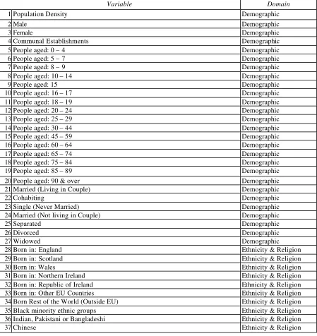
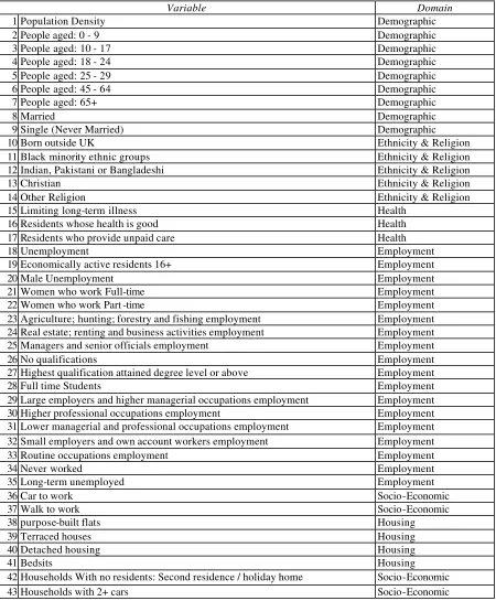
A comprehensive list of list of 129 variables was selected (see table 2), by reviewing
variables used in previous classification systems and adding variables which had been
[image:18.596.73.522.270.746.2]introduced in the 2001 census for the first time.
Table 2 The 129 variables considered for use in the LA Classification
Variable
Domain
1 Population Density
Demographic
2 Male
Demographic
3 Female
Demographic
4 Communal Establishments
Demographic
5 People aged: 0 – 4
Demographic
6 People aged: 5 – 7
Demographic
7 People aged: 8 – 9
Demographic
8 People aged: 10 – 14
Demographic
9 People aged: 15
Demographic
10 People aged: 16 – 17
Demographic
11 People aged: 18 – 19
Demographic
12 People aged: 20 – 24
Demographic
13 People aged: 25 – 29
Demographic
14 People aged: 30 – 44
Demographic
15 People aged: 45 – 59
Demographic
16 People aged: 60 – 64
Demographic
17 People aged: 65 – 74
Demographic
18 People aged: 75 – 84
Demographic
19 People aged: 85 – 89
Demographic
20 People aged: 90 & over
Demographic
21 Married (Living in Couple)
Demographic
22 Cohabiting
Demographic
23 Single (Never Married)
Demographic
24 Married (Not living in Couple)
Demographic
25 Separated
Demographic
26 Divorced
Demographic
27 Widowed
Demographic
28 Born in: England
Ethnicity & Religion
29 Born in: Scotland
Ethnicity & Religion
30 Born in: Wales
Ethnicity & Religion
31 Born in: Northern Ireland
Ethnicity & Religion
32 Born in: Republic of Ireland
Ethnicity & Religion
33 Born in: Other EU Countries
Ethnicity & Religion
34 Born Rest of the World (Outside EU)
Ethnicity & Religion
35 Black minority ethnic groups
Ethnicity & Religion
36 Indian, Pakistani or Bangladeshi
Ethnicity & Religion
38 White
Ethnicity & Religion
39 Christian
Ethnicity & Religion
40 Other Religion
Ethnicity & Religion
41 Not Stated or No Religion
Ethnicity & Religion
42 Limiting long-term illness
Health
43 Residents whose health is good
Health
44 Residents whose health is fairly good
Health
45 Residents whose health is not good
Health
46 Residents who provide unpaid care
Health
47 Unemployment
Employment
48 Self-employed
Employment
49 Economically active residents 16+
Employment
50 Male Unemployment
Employment
51 Working Women ft
Employment
52 Women who work part-time
Employment
53 Agriculture; hunting; forestry and fishing employment
Employment
54 Mining, quarrying and construction employment
Employment
55 Manufacturing employment
Employment
56 Electricity; gas and water supply employment
Employment
57 Wholesale & retail trade; repair of motor vehicles employment
Employment
58 Hotels and catering employment
Employment
59 Transport, storage and communication employment
Employment
60 Financial intermediation employment
Employment
61 Real estate; renting and business activities employment
Employment
62 Public administration and defence employment
Employment
63 Education employment
Employment
64 Health and social work employment
Employment
65 Managers and senior officials employment
Employment
66 Professional occupations employment
Employment
67 Associate professional and technical occupations employment
Employment
68 Administrative and secretarial occupations employment
Emp loyment
69 Skilled trades occupations employment
Employment
70 Personal service occupations employment
Employment
71 Sales and customer service occupations employment
Employment
72 Process; plant and machine operatives employment
Employment
73 Elementary occupations employment
Employment
74 No qualifications
Employment
75 Highest qualification attained level 1
Employment
76 Highest qualification attained level 2
Employment
77 Highest qualification attained level 3
Employment
78 Highest qualification attained level 4/5
Employment
79 Full time Students
Employment
80 Large employers and higher managerial occupations employment
Employment
81 Higher professional occupations employment
Employment
82 Lower managerial and professional occupations employment
Employment
83 Intermediate occupations employment
Employment
84 Small employers and own account workers employment
Employment
85 Lower supervisory and technical occupations employment
Employment
86 Semi -routine occupations employment
Employment
87 Routine occupations employment
Employment
88 Never worked
Employment
89 Long-term unemployed
Employment
91 Bus, Mini Bus or Coach to work
Socio-Economic
92 Car to work
Socio-Economic
93 Motorcycle, Scooter or Moped to work
Socio-Economic
94 Walk to work
Socio-Economic
95 Bike to work
Socio-Economic
96 Work mainly from home
Socio-Economic
97 Purpose-built flats
Housing
98 Terraced houses
Housing
99 Detached housing
Housing
100 Semi -detached Housing
Housing
101 Bedsits
Housing
102 Households With no residents: Vacant
Housing
103 Households With no residents: Second residence / holiday home
Housing
104 Caravan or other mobile or temporary structure
Housing
105 Households with 3+ cars
Socio-Economic
106 Households with 2 cars
Socio-Economic
107 Households with 1 car
Socio-Economic
108 No car households
Socio-Economic
109 Average number of cars per household
Socio-Economic
110 LA Rented
Housing
111 Owner occupiers
Housing
112 Private Rented
Housing
113 Mortgaged
Housing
114 Household size
Housing
115 Rooms per household
Housing
116 No central heating
Housing
117 Lacking bath, shower and toilet
Housing
118 Households: with an occupancy rating of -1 or less (Overcrowding)
Household Composition
119 One-person no-pensioner households
Household Composition
120 Single pensioner households
Household Composition
121 Wholly student households
Household Composition
122 2 adults no children
Household Composition
123 Only Pensioner households
Household Comp osition
124 Households with dependent children
Household Composition
125 Lone Parent Families
Household Composition
126 Households: With one or more person with a limiting long-term illness
Household Composition
127 Households: No adults in employment :with dependent children
Household Composition
128 Male lone parents
Household Composition
129 Population change 1991 – 2001
Demographic
N.B. Migration data could not be used, as it has not yet been published for Northern Ireland at the time when the classification was created.
These 129 variables needed to be assessed in terms of how much information they contain
about the areas and the inter correlations within the data, this will enable the reduction of the
list of variables whilst keeping as much information as possible.
Classification and Principal Components Analysis (PCA) are aspects of “social area analysis”
which are two sides of the same coin. The attention each has received has fluctuated over the
influence over the data; a correlation matrix can then be used to locate and remove high
levels of correlation within the data. Alternatively many commercial firms prefer to use a
strict PCA and cluster the components which are produced. Those components which
represent the first 90% of the variance within the data are selected to be used in the cluster
analysis. Each method is likely to produce slight variations in the final list of variables used
in the cluster analysis.
It was decided that the most suitable method of variable selection for this project was to use
the original variables rather than using PCA to produce surrogate variables. The
interpretation of the results is easier when the original variables are used rather than
composite components. However, PCA can play an important part in the selection of which
variables to keep and which to throw away. PCA was run using the SPSS statistical package
on the 129 variables producing both a 'component loadings matrix' and a 'correlation matrix'.
The component matrix was studied first; this is a matrix showing how much of the variance
of a variable was accounted for by each principal component. Variables which had a large
amount of their variance covered by the early principal components will be those variables
that are likely to have the most significance within the data and drive the classification. The
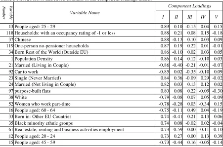
component loadings of first five principal components for the variables that have the greatest
amount of their variance associated with component one is shown in Table 3. The component
loading is the correlation between a variable and a component. Variables that have a large
amount of their variances covered by the first few principal components shows that a variable
[image:22.596.71.522.98.396.2]
(23)Table 3 First 20 Rows and first 5 columns of the component loadings matrix
Component Loadings
Variable
Number
Variable Name
I
II
III
IV
V
13 People aged: 25 - 29
0.89 0.10 -0.15 0.04 0.15
118 Households: with an occupancy rating of -1 or less
0.88 0.21 0.08 0.15 -0.18
37 Chinese
0.88 -0.13 0.10 0.03 0.09
119 One-person no-pensioner households
0.87 0.19 0.22 0.01 -0.01
34 Born Rest of the World (Outside EU)
0.86 -0.10 0.02 0.03 0.05
1 Population Density
0.86 0.14 0.12 -0.10 0.03
21 Married (Living in Couple)
-0.86 -0.40 -0.21 -0.01 -0.07
92 Car to work
-0.85 0.02 -0.35 -0.10 0.09
23 Single (Never Married)
0.84 0.36 -0.09 0.29 -0.02
24 Married (Not living in Couple)
0.82 0.03 0.13 0.12 0.02
97 purpose-built flats
0.80 0.08 0.22 -0.09 -0.30
38 White
-0.79 -0.08 0.07 0.05 -0.09
52 Women who work part-time
-0.78 -0.28 0.03 -0.34 0.15
16 People aged: 60 - 64
-0.75 -0.11 0.49 0.04 -0.19
33 Born in: Other EU Countries
0.74 -0.41 0.21 0.13 0.06
35 Black minority ethnic groups
0.74 0.08 -0.02 0.02 -0.04
61 Real estate; renting and business activities employment
0.73 -0.59 0.00 -0.11 -0.10
12 People aged: 20 - 24
0.73 0.27 0.00 0.13 0.39
15 People aged: 45 - 59
-0.73 -0.44 0.16 -0.05 -0.14
As well as establishing which variables power the dataset it is important to consider the
correlations between variables. There is no sense in having two highly correlated variables as
they will add little data to the classification. There are two different types of correlation
between variables. Variables that are positive represent characteristics of people which are
likely to be present in a person due to the type of person that they are, e.g. a student is likely
to be in their late teens or early twenties therefore the full time student variable will be
positively correlated with the age variable in which they fall as a large number of people who
are in one group are likely to be in the other. Negative correlations occur between variables
which represent characteristics that are unlikely to be present in a person for example people
over 65 years of age are highly unlikely to be full time students therefore these two variables
will high a high negative correlation. Negative correlations can also appear between variables
within the same domain, an example of this is age groups. Age groups at opposite extremes
i.e. young and old will be negatively correlated as an individual can only be of one age and
therefore can only be in one of the groups. Areas with high numbers of old people are likely
to have a low number of young people and this would make these two groups of people
0 - 4 5 - 7 8 - 9 10 -
14
15
16 -
17
18 -
19
20 -
24
25 -
29
30 -
44
45 -
59
60 -
64
65 -
74
75 -
84
85 -
89
90+
Age
X
0.84 0.68
0.55 0.45 0.47 0.15 0.27 0.49 0.56
-0.60 -0.75 -0.77 -0.72 -0.66 -0.61
0 - 4
X
0.91 0.81 0.70 0.67
0.05 -0.04 0.07 0.29 -0.31 -0.45 -0.51 -0.55 -0.57 -0.53
5 - 7
X
0.90 0.79 0.74
0.05 -0.13 -0.10 0.14 -0.18 -0.29 -0.37 -0.44 -0.52 -0.48
8 - 9
X
0.92 0.88
0.09 -0.20 -0.25 -0.08 -0.07 -0.13 -0.22 -0.31 -0.41 -0.39
10 - 14
X
0.92
0.16 -0.15 -0.24 -0.14 -0.07 -0.09 -0.18 -0.28 -0.38 -0.37
15
X
0.21 -0.09 -0.17 -0.13 -0.11 -0.14 -0.23 -0.32 -0.39 -0.37
16 - 17
X
0.81
0.29 -0.08 -0.54 -0.43 -0.36 -0.30 -0.29 -0.29
18 - 19
X
0.72
0.27
-0.78 -0.69
-0.58 -0.45 -0.37 -0.37
20 - 24
X
0.69
-0.78 -0.80 -0.76 -0.64
-0.52 -0.49
25 - 29
X
-0.42
-0.70 -0.78 -0.78 -0.68 -0.62
30 - 44
X
0.79 0.61
0.47 0.41 0.39
45 - 59
X
0.91 0.74 0.62
0.57
60 - 64
X
0.91 0.78 0.73
65 - 74
X
0.93 0.88
75 - 84
X
0.97
85 - 89
[image:23.596.55.524.85.323.2]X
90+
Figure 1 Correlation matrix of age variables
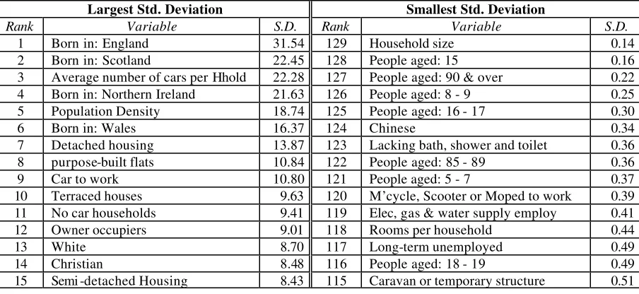
In addition to the correlations between the variables another thing that needs to be considered
is the variance of the variable across all local authorities. One way of doing this is to
compare the standard deviation of each variable, so that the variables which show the biggest
differences between the LAs are identified. The variables with the highest and lowest
standard deviation can be seen in table 4, which shows how different the standard deviation
can be for each variable ranging from as high as 31.54 down to 0.14.
Table 4 The variables with the highest and lowest standard deviation across all local authorities
Largest Std. Deviation
Smallest Std. Deviation
Rank
Variable
S.D.
Rank
Variable
S.D.
1
Born in: England
31.54
129
Household size
0.14
2
Born in: Scotland
22.45
128
People aged: 15
0.16
3
Average number of cars per Hhold
22.28
127
People aged: 90 & over
0.22
4
Born in: Northern Ireland
21.63
126
People aged: 8 - 9
0.25
5
Population Density
18.74
125
People aged: 16 - 17
0.30
6
Born in: Wales
16.37
124
Chinese
0.34
[image:23.596.68.520.521.729.2]It is much more reliable to use all of the different methods of selection as mentioned above.
Using just one you can make a case for most variables e.g. Chinese that has 88% of its
variance represented by Principal Component One suggesting that it could be an important
variable. However it has the 6
thlowest standard deviation showing that it varies very little
between local authorities and is therefore unlikely to add significant value to the
classification in terms of separating local authority areas into dissimilar clusters.
It is also important to consider which variable domains are covered by the variables that have
been selected. The Classifications also vary greatly in the variables that are used to make the
classifications. As there are so many different variables that have been used in the
classifications it was essential to group the variables in some way to enable a meaningful
comparison between them. The purpose of the investigation is to capture the complete
spectrum of people’s lives, living arrangements and problems. Therefore the classification
can be seen as being based on people’s
‘socio-economic life course’
in which, each person
experie nces a sequence of several parallel
‘careers’
during their lifetime. The variables used
in the classifications can be split into separate domains each representing a different
‘career’
within the
‘socio-economic life course’.
The variables within the classification were split in
seven domains or
‘careers’
that represent different types of variables. The seven domains
covered by the variables have been named: Demographic, Employment, Ethnicity &
Religion, Household Composition, Health, Housing, and Socio-Economic. Variables from
each of these domains need to be included in the final variable list to ensure that many
different types of data representing different characteristics of the people who live within
each local authority.
After all the criteria for reducing the variable list had been considered a final list of 56
variables was produced. So, 73 variables were either dropped from the list or merged with
another variable to create a less specific variable. The variables along with the reason behind
their inclusion or non inclusion are listed in Appendix A. The final list of variables used can
be found in table 5. The references for the calculation of the final 56 variables from the Key
In general an attempt was made to reduce the list of 129 as much as possible but with losing
as little as possible of the information they contain. To do this variables that show extremes
within the population have been treated as the most important variables to keep as they are
[image:25.596.73.523.204.749.2]the most likely to distinguish between areas.
Table 5 The final list of 56 variables to be used in the classification.
Variable
Domain
1 Population Density
Demographic
2 People aged: 0 - 9
Demographic
3 People aged: 10 - 17
Demographic
4 People aged: 18 - 24
Demographic
5 People aged: 25 - 29
Demographic
6 People aged: 45 - 64
Demographic
7 People aged: 65+
Demographic
8 Married
Demographic
9 Single (Never Married)
Demographic
10 Born outside UK
Ethnicity & Religion
11 Black minority ethnic groups
Ethnicity & Religion
12 Indian, Pakistani or Bangladeshi
Ethnicity & Religion
13 Christian
Ethnicity & Religion
14 Other Religion
Ethnicity & Religion
15 Limiting long-term illness
Health
16 Residents whose health is good
Health
17 Residents who provide unpaid care
Health
18 Unemployment
Employment
19 Economically active residents 16+
Employment
20 Male Unemployment
Employment
21 Women who work Full-time
Employment
22 Women who work Part -time
Employment
23 Agriculture; hunting; forestry and fishing employment
Employment
24 Real estate; renting and business activities employment
Employment
25 Managers and senior officials employment
Employment
26 No qualifications
Employment
27 Highest qualification attained degree level or above
Employment
28 Full time Students
Employment
29 Large employers and higher managerial occupations employment
Employment
30 Higher professional occupations employment
Employment
31 Lower managerial and professional occupations employment
Employment
32 Small employers and own account workers employment
Employment
33 Routine occupations employment
Employment
34 Never worked
Employment
35 Long-term unemployed
Employment
36 Car to work
Socio-Economic
37 Walk to work
Socio-Economic
38 purpose-built flats
Housing
39 Terraced houses
Housing
40 Detached housing
Housing
41 Bedsits
Housing
44 No car households
Socio-Economic
45 LA Rented
Housing
46 Private Rented
Housing
47 Household size
Household Composition
48 No central heating
Housing
49 Households: with an occupancy rating of -1 or less (overcrowding)
Household Composition
50 One-person no-pensioner households
Household Composition
51 Single pensioner households
Household Composition
52 2 adults no children
Household Composition
53 Households with dependent children
Household Composition
54 Lone Parent Families
Household Composition
55 Households: No adults in employment :with dependent children
Household Composition
56 Population change 1991 - 2001
Demographic
5.2 Clustering the Local Authorities
The method that was used for clustering the variables was Ward’s Hierarchical Grouping
Procedure also known as the Increased Sums of Squares Method. Developed by Joe H. Ward
of the Aerospace Medical Division, Lockland Air Force Base, it was first published in the
Journal of the American Statistical Association in 1963, and developed as a method
“to
cluster large numbers of objects, symbols or persons into smaller numbers of mutually
exclusive groups, each having members that are as much alike as possible”
(Ward 1963
pp236), the aim is to join objects together into ever increasing sizes of cluster using a
measure of similarity or distance. Cluster membership is assessed by calculating the total sum
of squared deviations from the mean of a cluster. The criterion for fusion is that it should
produce the smallest possible increase in the error sum of squares (ESS).
The clustering procedure forms groups in a manner that minimizes the loss associated with
each grouping and to quantify that loss in readily interpretable form. Information loss is
defined by Ward in terms of an error sum-of-squares (ESS) criterion. ESS is defined as the
following:
ij
x
= Value for area
i
of variable
j
k
= index for clusters,
k
=
1
,...,
K
k
i
= index of an area,
i
=
1
,...,
N
j
= index for variables,
j
=
1
,...,
M
j
= number of areas in the cluster
The Sum of Squared deviations from the mean for cluster
k
is
2
1
)
(
ij kjM j D i
k
x
x
SS
k
−
=
∑
∑
= ∈
(7)
Where
x
kj=
mean of
x
ijfor all
i
in cluster
k
=
∑
∈Dk i k
ij
n
x
The Sums of Squared Deviation
(SS
)
for cluster
k
is given as:
∑∑∑
∈ =−
k i D M j
kj ij k
x
x
12
)
(
(8)
and the Error Sums of Squared deviations
(ESS
)
is simply the sum across all clusters
ESS
=
∑
k k
SS
(9)
The process of hierarchical clustering is an agglomerative or (bottom- up) approach beginning
with
n
groups each containing 1 object which are merged together ending with 1 group
containing
n
objects. The process of getting from
n
to 1 groups can be summarised by the
following 5 steps:
Step 1:
Place each object
O
into its own cluster
C
, creating the cluster file
f
therefore:
1 2 3 2
1
,
,...,
,
,
,
C
C
C
C
C
C
f
=
n n− n−Step 2:
Compute a measure of similarity between every pair of clusters in the cluster file
f
to find the closest pair
{
C
i,
C
j}
Step 4:
Merge
C
iand
C
jto create a new cluster
C
ijwhich will be the parent of
C
iand
j
C
in the hierarchical cluster tree.
Step 5:
Return to step 2 and repeat until there is only one cluster left.
Methods of hierarchical clustering have been incorporated into the Statistical Package for the
Social Sciences (SPSS) and are frequently used to cluster census type information. There are
several different formulae that can be used as the criterion in a hierarchical grouping
procedure, most commonly used is Euclidean distance (SPSS 1999).
Assume two objects
i
=
i
1,
i
=
i
2Assume two variables
j
=
j
1,
j
=
j
2Assume the distance is given by the Pythagorean formula (square of the hypotenuse = sum of
the squares on the other two sides of a right angle triangle)
then the distance between the objects is
2 1 2 2
}
)
(
)
{(
2 2 2 1 1
2 1 1 2
1i ij ij ij i j
i
x
x
x
x
d
=
−
+
−
(10)
object
i
1variable
j
11
2
j
x
i1
1
j
x
i2
2
j
x
i2
1
j
x
iobject
i
2Generalising over variables this becomes
2 1 2 1}
)
(
{
2 1 2 1∑
=−
=
M j j i j i ii
x
x
d
(11)
The distances between clusters can then be calculated, the Intra-cluster distance involves
generalising over objects
i
which are members of cluster
k
∑ ∑ ∑
∈ ∈ =
−
=
k i i k
M j j i j i
kk
x
x
d
1 2 2 1 1 2 1 2}
)
(
{
(12)
Inter-cluster distance is then defined as
∑ ∑ ∑
∈ ∈ =
−
=
1
1 2 2
2 1 2 1 1 2 1 2
}
)
(
{
k i i kM j j i j i k
k
x
x
d
(13)
Once the variables have been clustered the next decision that has to be made is how many
clusters to split the LAs into. Unlike other methods of clustering such as k- means, the Ward’s
method clustering used does not have to be provided with predefined a number of clusters.
Instead a range of solution is produced, from 434 clusters where all LAs are in separate
groups, to just 2 clusters. In total this gives 433 different classifications of the LAs so some
method of selecting the most suitable number of clusters to use is needed. It is important as
well to remember that the cluster in procedure is hierarchical so a multiple level classification
system can be produced.
The ONS classification of local authorities of Great Britain using 1991 data produced a three
tier hierarchy of 27, 15 and 7 clusters (Bailey et al. 1999). Using the ONS classification as a
guide the aim will be to produce a three tier hierarchy with the number of clusters more or
less doubling with each tier hopefully ending in the tier with between 25 – 30 clusters e.g.
(28, 14 and 7). However knowing the structure would work best theoretically does not mean
that they will be the must suitable number of clusters in reality for the data that has been
used. The method used to choose the clusters the number of clusters was to examine the
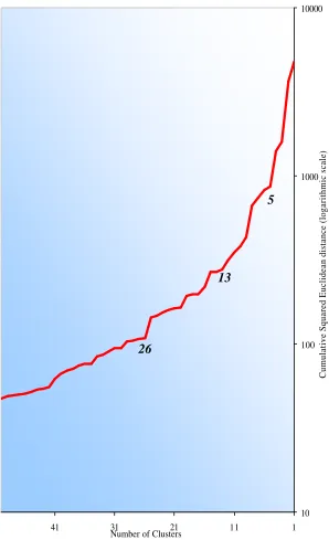
relative increase in the sum of squares. The tiers that are suitable for selection are those that
where the sum of squares shows a sharp rise immediately afterwards, therefore those tiers
classification were chosen the graph clearly shows a significant increase in the sums of
squares immediately after the tiers with 26, 13 and 5 clusters.
10 100 1000 10000
1 11
21 31
41
Number of Clusters
[image:30.596.161.459.142.631.2]Cumulative Squared Euclidean distance (logarithmic scale)