Infinities of stable periodic orbits in systems of coupled oscillators

oscillators

.

White Rose Research Online URL for this paper:

http://eprints.whiterose.ac.uk/177/

Article:

Ashwin, P., Rucklidge, A.M. and Sturman, R. (2002) Infinities of stable periodic orbits in

systems of coupled oscillators. Physical Review E, 66 (3 (art). pp. 1-4. ISSN 1063-651X

https://doi.org/10.1103/PhysRevE.66.035201

[email protected] https://eprints.whiterose.ac.uk/

Reuse

See Attached

Takedown

If you consider content in White Rose Research Online to be in breach of UK law, please notify us by

stable periodic orbits that accumulate on the cycling, whereas for a free-running example loss of stability of the cycling gives rise to a single quasiperiodic or chaotic attractor.

DOI: 10.1103/PhysRevE.66.035201 PACS number~s!: 05.45.Ac, 05.45.Xt, 47.52.1j

Physical systems where an invariant subspace, or set of subspaces, are preserved because of symmetry or other con-straint give rise to a number of new types of robust behavior

~i.e., behavior that is robust to perturbations that preserve the structure!that would be highly degenerate for systems with-out the symmetry or constraint. There is an extensive litera-ture discussing theory and examples of this for a variety of physical problems@1#.

Structurally stable heteroclinic cycles between equilibria are well documented in ordinary differential equations with symmetries. Examples have been found in many applications such as rotating convection and population dynamics @2#, where the system repeatedly spends long periods of time near one equilibrium state, then rapidly switches to another. Heteroclinic cycles between chaotic saddles are also robust in systems with symmetry; these have been found in coupled oscillators@3# and models of planar magnetoconvection@4#, the latter example being a cycle alternating between equilib-ria and chaotic saddles. This kind of behavior arises in many symmetric physical systems of sufficient complexity. In coupled oscillator examples, initially one oscillator is active

~it could be periodic or chaotic! while the others are sup-pressed; later, one of these becomes active and quenches the original active oscillator, and so on. This phenomenon is the counterpart of synchronization.

By analogy with cycles between equilibria for flows, whether such cycling between periodic orbits or chaotic saddles is an attractor or not can be determined by examining the ratios of Lyapunov exponents at the saddles @4,5#. The cycling loses stability at a bifurcation which occurs when rates of linear expansion and contraction become equal ~a resonance of Lyapunov exponents!. Numerical simulations in Ref. @4# suggest that such a resonance creates a large number of periodic attractors that branch from the cycling chaos. By contrast, for the skew-product example of cycling chaos examined in Ref.@5#the resonance was found to give

rise not to periodic orbits but to a chaotic attractor with av-erage cycling chaos, or to quasiperiodicity that is intermittent

~stuck on!to the cycling chaos.

In this note, we aim to reconcile these differences by char-acterizing them as examples of qualitatively different types of cycling. For what we call ‘‘phase-resetting’’ cycling, there is only one approach trajectory towards each saddle within the cycle, while in ‘‘free-running’’ cycling, there are multiple approaches to a single saddle.

We consider two systems of coupled iterated maps where the attraction of the cycling is determined by the strength of the coupling. These maps can be related to flows in the usual way via a Poincare´ return map, noting that equilibria and periodic points for a map both correspond to periodic orbits for a flow.

At the resonance bifurcation, for the phase-resetting case we find a plethora of stable high-period periodic orbits with an infinite number of stable periodic orbits accumulating at resonance. For the free-running case the branching attractors are typically unique and quasiperiodic or chaotic. We ob-serve no other scenarios for these models but believe there will be other scenarios for problems with higher dimensional saddles and connections.

Model I is a map of@0,1#3 _with

Z3 symmetry given by

~xn11, yn11,zn11!5FI~xn, yn,zn!,

where

FI~x,y ,z!5„f~x!e2gz, f~y!e2gx, f~z!e2gy…,

and f (x)₅rx(1₂x) denotes the logistic map with parameter r. This map clearly preserves the coordinate planes x y z 50. In each variable three distinct types of evolutions are possible. For example, consider x: if z_!1 and x_!1 then x grows approximately linearly—the growing phase. For z !1 and x'O(1), x evolves according to logistic map dynamics—the active phase. Finally if z'O(1) the dynam-ics in the x direction is suppressed by the coupling term—the decaying phase.

*Email address: [email protected] †_{Email address: [email protected]}

Model II is identical to Model I except that the logistic map f during a growing phase is replaced by f˜,

f˜~xn!5

H

f~x_n!, x_n,e or x_n.f~e!

f2_~e!

5h, x_nP@e, f~e!#.

Each time a growing variable reaches the interval @e, f (e)# ~we usee51026), it is set toh5f2(e). From this point on, all trajectories then evolve in an identical way. The interval

@e, f (e)# is of sufficient size to ensure that all trajectories visiting xn,ein the growing phase are reset in this way. The

effect of the resetting is to force trajectories leaving one saddle to approach the next one close to a single trajectory. This is observed in cycling that alternates between equilibria and chaos for flows @4#. To ensure that e_,f (e) we take r

P@1/(12e),4#.

For both models the coupling is trivial wheng₅0. When the coupling parameterg is sufficiently strong both the mod-els exhibit robust cycling between invariant sets. In this state, each variable alternates cyclically between the growing, the active, and the decaying phases. We term a change in the phases a ‘‘switch.’’ More precisely, we say a switch occurs when the growing variable exceeds ln r/g. Figure 1 shows a time series for Model I of the three variables cycling, illus-trating the three possible phases and the switches between them. As in Ref. @4#, for both the models, the number of iterations between switches increases geometrically as trajec-tories approach the invariant subspaces, and this rate of in-crease depends on the coupling g. The rate of increase of switching times approaches zero asg approaches some criti-cal value from above, which forms the limit of the stability of cycling chaos. Referring to Fig. 1, decreasing g would result in a slower rate of increase in the number of iterations between switches, and the line formed by connecting the local minima would become more horizontal.

The behavior in the active phase is governed by r. For r ,3 the cycles are between period one points; as r is in-creased ~after period doubling! we obtain cycles

progres-sively between periodic orbits and then chaotic saddles. Since numerical simulations of this system need to resolve a neighborhood of the invariant subspaces very clearly, we use logarithmic coordinates@4#. The time series in Fig. 1 is for parameters that produce attracting cycling chaos; Model II produces similar behavior at this parameter value.

Suppose that cycling chaos loses stability on decreasingg through a critical valuegc. We can computegcanalytically,

either from a resonance condition of Lyapunov exponents, or as follows. Suppose that a switch has just occurred and the growing variable is z, so z_!1, x is O(1) and y is decaying. The evolution of z is governed by z_n115rzn(12zn)e2gyn,

and this can be approximated by z_→rz. Starting at a switch at z₅z0, suppose that the number of iterations until the next switch is N. Then zN'rNz0, and since zN is O(1) at a

switch, N'₂ln z₀/ln r. While z is growing, y is decaying, and for critical g we require yN5z0. We approximate yN in

a similar way, with y0 an O(1) number. Throughout the decay phase y_!1 but it is forced by the active variable x. Here we approximate by y→r y e2gx, and replace x by its

long-term average A`@5limm→`(1/m)(i50

m21

fi(x0)#for each of the N iterations, giving yN'rNe2gNA`. Then substituting

our expression for N, we have ln yN'2ln z0 1(gln z0A`)/(ln r). The critical value of g occurs when yN

5z0, givinggc52 ln r/A`. The average A` is easy to

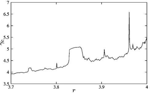
com-pute numerically, and so we obtain a curve of critical g shown in Fig. 2. The criticalg for Model II can be found as for Model I because the dynamics in the invariant subspace y5z50 and its linearization about that subspace is identical to Model I.

One of the questions raised in Ref. @4# is what sort of attractors branch from cycling chaos at resonance. In that paper, numerical evidence was presented suggesting that the cycling chaos gives way to families of long-period periodic orbits made up of repeated segments of a single chaotic tra-jectory. In Model I this does not occur; for g,gc we find

irregular cycling in which the number of iterations between switches behaves erratically. Model II, like Model I, exhibits attracting cycling above the resonance value gc. However, FIG. 1. Attracting cycling chaos, with r54.0, g56.0. Model I

is iterated and x,y ,z plotted ~in logarithmic coordinates! against time. The chaotic behavior is O(1) and is visible in the inset. The trajectory cycles through growing, active, and then decaying phases for each variable, with the length of phase increasing approximately geometrically. The same behavior is found for Model II.

FIG. 2. The critical value of g at which loss of stability of cycling chaos occurs for Models I and II. Above the line, the cy-cling is an attractor; below the line the cycy-cling persists but is no longer an attractor.

PETER ASHWIN, ALASTAIR M. RUCKLIDGE, AND ROB STURMAN PHYSICAL REVIEW E 66, 035201~R! ~2002!

forg,gcwe find existence of many periodic orbits,

consist-ing of cycles between either periodic points or chaotic tra-jectories ~depending on the value of r). We argue that this multistability of long-period orbits is caused by, and is typi-cal for, cycling with phase-resetting approach to chaotic saddles.

For the remainder of this note, we investigate these peri-odic orbits by carefully considering the evolution of the vari-ables over one third of a periodic orbit as shown in Fig. 3.

~Throughout, the period of the orbit will be 3N.!We assume that x has just reset to x_n5h at n₅0, so that y is the active variable and z is in the decay phase. For a periodic orbit of period 3N to be possible, we require that zN5h—i.e., that

z_N21P@e, f (e)#. We take yk5a, where a is either some

O(1) number A¯ ~for a rough estimate!, or more precisely takes the value fN1k(h) @since y05xN'fN(h)]. There

fol-low N iterates of forced decay. We approximate this by y_N1k5rN_y

ke2gNb, where b approximates the suppressing

effect of the forcing. Again, for a rough estimate, we takeb to be the long-term average A_`, but for a more accurate

estimate we take b to be the N average AN

51/N(_i5N2₀1

fi@fk(h)#. Since this is a periodic orbit, yN1k

5zk5rNae2gNb. Finally we have (N2k21) iterations of

growth, approximated by z_→rz. This gives z_N21 5r2N2k21_ae2gNb_{. Taking logarithms, this estimate predicts}

that a periodic orbit will exist when

lne,~2N₂k₂1!ln r₁lna2gNb,lne1ln r,

that is, for the rough estimatea5A¯ , b5A_`, for

N_P@N1,N2#5

F

a1ln r 2 ln r₂gA_`

G

where a₅lne2ln A¯₁(k₁1)ln r. This defines a pair of hyper-bolas between which N must lie for a periodic orbit to exist, and suggests that all N_P@N1,N2# should be present. Bothe and r are fixed, and k ~the number of iterations from the resetting point to the next switch! can be calculated. To es-timate the latter, we consider the number of iterations to take x05h to xk.ln r/gunder the approximation xn115rxn

giv-ing k'@ln(ln r/gh)#/ln r. In other words, the hyperbolas are governed by a single fitting parameter A¯ . Note that the

de-nominators in these expressions equal zero when g 52 ln r/A`5gc. Such a pair of hyperbolas can be seen in the

inset of Fig. 4.

This estimate works well for the case in which the active phase of the maps is a period one point—i.e., for r_,3. Nu-merically located periodic orbits lie within the predicted hy-perbolas. In particular, for a giveng we obtain all periods for N between N1and N2 with a suitable choice of A¯ . For more complicated behavior within the invariant subspaces this es-timate works less well. As r is increased the logistic map undergoes period doubling. For values of r in this region the numerically located periodic orbits still lie roughly between the predicted hyperbolas. However, we no longer find all periods for N in@N1,N2#: some are not present near N1 and N2.

As r increases further, the saddles become chaotic and the bifurcation diagram of periodic orbits gets more compli-cated. In this case we use the improved estimate with a 5fN1k(h), b5AN. This gives the estimate

z_N215r2N2k21_fN1k_~h!e2gNA_{N. ~1!}

For fixed r, g, e, andh, zN21 is a function only of N and there are no free parameters. Figure 4 plots this estimate of ln z_N21for different N for r53.1, and shows how it success-fully predicts periodic orbits when the line falls within the band defined by@lne,lne1ln r#. The squares on the diagram represent actual periodic orbits. The inset shows the hyper-bolas from the simple approximation.

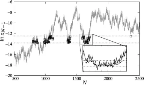
For values of r that give chaotic dynamics within invari-ant subspaces, the situation is more complicated, but the im-proved approximation still does a good job of predicting pe-riodic orbits. The approximation for zN21is plotted in Fig. 5 for r₅3.75 andg54.01. Figure 6 is a bifurcation diagram of periodic orbits present for the chaotic case r₅3.75, together with the predicted envelope. The actual periodic orbits fit well inside the prediction, with the exception of some

longer-Model II; one third of a period is shown. This is a periodic orbit as the final and initial phases match up as shown. The iterate k shows

where the phases switch. FIG. 4. Predicted and actual period 3N orbits for r53.1, g

53.495 for Model II. The squares indicate the location of periodic orbits, the line is the improved approximation of zN21: if it lies in the band@e,re# we predict that the resetting will lead to a stable periodic orbit. The inset shows the hyperbolas ~plotted as lines!

period orbits lying above the envelope. These tend to be orbits that just fail to join up and make a period 3N orbit, but instead become periodic after 6N iterations. Using this method to create an envelope not only gives a good way to predict the location of periodic orbits, but again makes clear that upon approachinggcwe expect to find periodic orbits of

increasing period. For g5gc the chaotic curve of ln zN21 against N neither increases nor decreases on average~cf. Fig. 5!, but the fluctuations, driven by the NAN term in Eq.~1!,

can be expected to increase. Hence we expect periodic orbits of arbitrarily high period as the curve repeatedly crosses the band@e,re#. Forg close togc~above or below!the

fluctua-tions for N large lead to possible long-periodic orbits, but eventually the linear average behavior leads the curve away from the band.

In the phase-resetting case~Model II!, the qualitative dy-namics is independent of the value ofh. The presence of the multiplicity of periodic orbits presents an intriguing parallel between this model and the persistent phenomenon of ‘‘Newhouse sinks’’ in a neighborhood of a homoclinic tan-gency@6#. One difference is that even in the simpler case of robust cycling between periodic points in Model II, the tan-gency between unstable and stable manifolds will be degen-erate owing to the invariant manifolds containing the

con-nections. Another difference is that the stable periodic orbits in this case are easy to locate numerically and indeed there appear to be no other attractors nearby. The mechanism that creates the periodic orbits in Model II resembles that found by Chawanya@7#near a robust heteroclinic network contain-ing connections to a heteroclinic cycle. Model II is artificial in that it has a discontinuity at the phase resetting step. This means that the periodic orbits typically bifurcate from this discontinuity in a degenerate way. However, one can clearly remove this problem by smoothing out the discontinuity.

In summary, we have demonstrated how the absence

~Model I! or presence ~Model II! of phase resetting in the connections between saddles of a cycling ~robust hetero-clinic!attractor can cause qualitatively different behaviors at loss of stability of the attractor by resonance of Lyapunov exponents, even though the behaviors for attraction are simi-lar. These models are instructive in that they are simple enough to allow a precise estimation of the location of peri-odic orbits while having what we believe are the main fea-tures of robust types of dynamical behavior in flows.

The research of P.A., A.R., and R.S. is supported by EPSRC Grant No. GR/N14408.

@1#A.S. Pikovsky and P. Grassberger, J. Phys. A 24, 19~1991!; H Fujisaka and T. Yamada, Prog. Theor. Phys. 69, 32~1983!; E. Ott and J.C. Sommerer, Phys. Lett. A 188, 39 ~1994!; J.C. Alexander, I. Kan, J.A. Yorke, and Z. You, Int. J. Bifurcation Chaos Appl. Sci. Eng. 2, 795~1992!; P. Ashwin, J. Buescu, and I. Stewart, Phys. Lett. A 193, 126 ~1994!; K. Kaneko, Phys. Rev. Lett. 78, 2736~1997!; S.C. Venkataramani, B.R. Hunt, E. Ott, D.J. Gauthier, and J.C. Bienfang, ibid. 77, 5361~1996!.

@2#M. Krupa, J. Nonlinear Sci. 7, 129~1997!; A.S. Kuznetsov and J. Kurths~unpublished!.

@3#M. Dellnitz, M. Field, M. Golubitsky, A. Hohmann, and J. Ma, IEEE Trans. Circuits Syst., I: Fundam. Theory Appl. 42, 821

~1995!.

@4#P. Ashwin and A.M. Rucklidge, Physica D 122, 134~1998!.

@5#P. Ashwin, Chaos 7, 207~1997!.

@6#J. Palis and F. Takens, Hyperbolicity and Sensitive Chaotic Dynamics at Homoclinic Bifurcations ~CUP, Cambridge, 1995!.

@7#T. Chawanya, Physica D 109, 201~1997!. FIG. 5. Predicted and actual periodic orbits for r53.75, g

54.01 for Model II. As in Fig. 4, squares represent stable periodic orbits and the line is the approximation of zN21.

FIG. 6. Period 3N stable periodic orbits for Model II with r

53.75 are marked by dots. The lines show the predicted envelope on varying the parameter g. The period of the periodic orbits ap-proaches infinity asg approachesgc54.061 167.

PETER ASHWIN, ALASTAIR M. RUCKLIDGE, AND ROB STURMAN PHYSICAL REVIEW E 66, 035201~R! ~2002!