Topics in Quantum Computing Architecture

(1)

Topics in Quantum Computing

Architecture

Thien Nguyen

Research School of Engineering

The Australian National University

A thesis submitted for the degree of

Doctor of Philosophy

College of Engineering and

Computer Science

May 2019

(2)

(3)

To my family:

(4)

(5)

Declaration

I hereby declare that except where specific reference is made to the work of others,

to the best of my knowledge and belief, the contents of this dissertation are original

and have not been submitted in whole or in part for consideration for any other degree

or qualification in this, or any other university. This dissertation is my own work or

partially in collaboration with others. This dissertation contains fewer than 100,000

words exclusive of appendices, bibliography, footnotes, tables and equations.

Thien Nguyen

(6)

(7)

Acknowledgements

In no way would this thesis have been possible without the support of many people who

guided and encouraged me along the way. First and foremost, I am much indebted to

my supervisors, Prof. Matthew James, who has been incredibly supportive from even

before my arrival at the ANU and remained so throughout my study. Matt gave me total

freedom to pursue my interests and helped me connect with experts in the field. At the

same time, he was constructively critical of various aspects of my study and professional

development.

I am grateful to Prof. Lloyd Hollenberg for taking an interest in me and giving

me an opportunity to work with him on the interesting problems of quantum computer

architecture. My special thanks also go to Dr Charles Hill. Charles’ eye for detail and

technical expertise has helped me in refining my ideas into research projects.

In the course of my study at the ANU, I have had the opportunity to work with and

learn from incredibly smart people to whom I would like to express my gratitude. They

are Dr Yu Pan, Dr Guodong Shi, Dr Shibei Xue, Dr Zibo Miao, Dr Shuangshuang Fu,

Dr Michael Hush, and Dr Andre Calvalho. I appreciated every conversation which I had

with every one of you, through which I have expanded my knowledge and understanding

of the quantum field.

To my fellow PhD students, Alfred, Oliver, Jessica, Alex, James, and Ruvi, it was

great listening to your talks in our group meeting. Special thanks to those who always

accepted my invitation to give a speech when I was the coordinator.

During my PhD, I have had the opportunity to work as a research intern at the Atos

Quantum Lab in Paris, France. To this, I’d like to thank Dr Cyril Allouche, head of

the Atos Quantum research program, and Sophie Houssiaux, head of R&D, Big Data

(8)

viii

research. I also want to express my thanks to the whole Atos quantum lab members who

taught me a lot about quantum computing, supercomputers, and especially about French

culture.

I am grateful to my wife who, despite struggling with her PhD study, has always

provided me emotional support whenever I need. Special thanks to my family members

in Vietnam, who have supported me along the way.

Last but not least, to every participant of the Friday lunch Quantum Cybernetics

group meeting, it was pleasant sharing lunch and discussing a wide variety of topics

with all of you during last four years.

I also gratefully acknowledge the generous financial support I have received from

(9)

Abstract

Quantum computing, which is considered the next revolution of computing technology,

brings together theories of mathematics, physics, and computer science. Building a

quantum computer thus requires a synthesis of knowledge and skills from multiple

disciplines. In this thesis, we take a step toward bridging and connecting the full “stack”

of quantum computing technology which spans across theoretical foundations, hardware

architecture, software and simulation.

At the foundation level, we study one of the central problems of quantum computing,

namely quantum error correction, from a control-engineering perspective. This approach

not only complements the conventional coding-based interpretation but also provides a

potential pathway to designing self-correcting quantum computers. First, we analyse

the surface-code quantum error correction under a continuous feedback-based protocol.

Second, we study the fundamental question of self-correcting quantum systems using

the control method of reservoir engineering.

Next, we study the scalability of a generic surface code quantum computer based on

spin qubits such as quantum dots and donor atoms. Solid-state qubits (quantum dots and

donor atoms), especially those that are Si-based, share similarities in device structures

and manufacturing processes with advanced semiconductor CMOS industry. However,

scaling up those quantum devices present immense challenges related to connectivity.

By applying tools and methods from the semiconductor industry, we can concretely

estimate the routing limitation of a planar connectivity scheme.

Finally, as part of my PhD education at the Australian National University, I took

part in an industry-based research internship to develop a high-performance quantum

simulator. We provide the full description of the software architecture, implementation

(10)

(11)

List of Publications

This thesis is based on the following collection of papers which have either been

published in or submitted to peer-reviewed journals or conferences. Some of this work

was completed jointly with other researchers and selections from these joint papers to be

included in this thesis are only those that this author contributed significantly towards.

Journal Publications

1. Thien Nguyen, Charles D. Hill, Lloyd C. L. Hollenberg, and Matthew R. James.

Fan-out Estimation in Spin-based Quantum Computer Scale-up. Scientific Reports

7, Article number: 13386 (2017)

2. Yu Pan and Thien Nguyen. Stabilizing Quantum States and Automatic Error

Correction by Dissipation Control. IEEE Transactions on Automatic Control

(Volume: 62, Issue: 9, Sept. 2017) Page(s): 4625 - 4630

3. Thien Nguyen, Zibo Miao, Yu Pan, Nina Amini, Valeri Ugrinovski, and Matthew

James. Pole placement approach to coherent passive reservoir engineering for

storing quantum information. Control Theory Technology (2017) 15: 193.

4. Shibei Xue, Thien Nguyen, Matthew R. James, Alireza Shabani, Valery

Ugri-novskii, Ian R. Petersen. Modelling and Filtering for Non-Markovian Quantum

Systems. Pre-print: arXiv:1704.00986

5. Yi Li, Thien Nguyen, and Yu Pan. Deterministic Multi-Party Quantum Key

(12)

xii

Peer-reviewed Conference Publications

1. Thien Nguyen, Charles D. Hill, Lloyd C. L. Hollenberg, and Matthew R. James.

Surface Code Continuous Quantum Error Correction Using Feedback. In

Proceed-ings of IEEE 54th Annual Conference on Decision and Control (CDC): Osaka,

Japan, December 2015

2. Yu Pan,Thien Nguyen, Zibo Miao, Nina Amini, Valeri Ugrinovski, and Matthew

James. Coherent observer engineering for protecting quantum information. In

Proceedings of the 35th Chinese Control Conference (CCC): Chengdu, China,

August 2016

3. Thien Nguyen, Zibo Miao, Yu Pan, Nina Amini, Valeri Ugrinovski, and Matthew

James. Pole placement approach to coherent passive reservoir engineering for

storing quantum information. In Proceedings of American Control Conference

(ACC): Seattle, WA, USA, July 2017

4. Shibei Xue, Thien Nguyen, and Ian R. Petersen. Feedback Control of a

Non-Markovian Single Qubit System. In Proceedings of the 11th Asian Control

(13)

List of figures

1.1 Qubit Bloch sphere . . . 5

1.2 Solid-state qubit diagram . . . 6

1.3 Quantum gate timing . . . 9

1.4 Quantum gate decomposition . . . 10

1.5 Surface code layout diagram . . . 13

1.6 Quantum circuit to measure surface code syndromes . . . 13

1.7 LogicalCNOT gate braiding diagram . . . 14

1.8 LogicalCNOT gate by braiding holes in surface code . . . 15

1.9 Active and passive QEC diagram . . . 19

1.10 Diagram of a typical quantum filtering set-up. . . 20

1.11 SLH network connections . . . 21

1.12 Diagram of beamsplitter in series with cavity QED. . . 22

1.13 Sample QHDL code . . . 23

1.14 Sample QHDL schematic . . . 24

1.15 Measurement feedback block diagram. . . 25

1.16 Coherent feedback block diagram. . . 26

1.17 Overall architecture of a universal quantum computer. . . 27

2.1 Routing parameters . . . 32

2.2 Diagram of surface code lattice with embedded readout devices . . . 34

2.3 Diagram of a generic surface code array unit cell . . . 35

2.4 Metal 1 pitch scaling roadmap from ITRS . . . 36

2.5 Ring-by-ring routing . . . 39

2.6 Layer optimal routing . . . 40

2.7 Illustration of 2-D qubit lattice surface gate fanout . . . 42

2.8 Fanout scalability at fixed interconnect length . . . 43

2.9 Qubit fanout scalability in terms of number of routing layers . . . 45

2.10 Fan-out scalability vs. interconnect length for SSI and ECI schemes . . . 46

3.1 Surface code layout diagram . . . 52

3.2 Distance-2 surface code . . . 56

(20)

xx LIST OF FIGURES

3.4 Syndrome estimation trajectories . . . 62

3.5 Continuous feedback error correction fidelity comparison . . . 63

3.6 Distance-3 surface code diagram . . . 64

3.7 Time-domain simulation of distance-3 surface code under continuous QEC . 66 3.8 Fidelity vs. feedback strength plot . . . 67

4.1 Potential function plot . . . 80

4.2 Lyapunov function scalability . . . 85

4.3 State evolution simulation of repetition error correction code . . . 97

4.4 Repetition error correction code under dissipative couplings . . . 98

4.5 Coherent feedback network for DFS generation. . . 100

4.6 Open loop setup for DFS generation. . . 101

4.7 Coherent plant-observer network . . . 109

4.8 Coherent feedback network for DFS generation . . . 111

4.9 Two-cavity system diagram . . . 115

5.1 AQASM example . . . 122

5.2 AQASM QFT example . . . 123

5.3 PyAQASM QFT example . . . 124

5.4 Quantum simulator diagram . . . 125

5.5 Path integral diagram . . . 127

5.6 Quantum circuit simulation objects . . . 128

5.7 Benchmark of Hadamard gates . . . 129

5.8 Comparison with Liquid . . . 130

5.9 Comparison with other simulators . . . 130

6.1 QHDL design flow . . . 135

6.2 Single-photon generating filter cascading realization. . . 136

6.3 Gradient settings for GEM operations . . . 137

6.4 Engineered dissipation by direct coupling . . . 139

6.5 Quantum circuit of cascading Hamiltonian unitary . . . 141

6.6 Discretized single-photon GEM model . . . 142

6.7 Amplitude damping LIQU i_|⟩code snippet . . . 143

6.8 Histogram of photon detection events . . . 144

6.9 Photon absorption vs. photon bandwidth . . . 145

B.1 OpenCL implementation of complex arithmetic . . . 177

(21)

List of tables

1.1 Types of experimental quantum bits (qubits) . . . 7

1.2 Hadamard gate implementation steps . . . 10

2.1 Gate count configurations for spin shuttling interconnect (SSI) and end control interconnect (ECI) protocols . . . 37

2.2 Minimum interconnect length for spin shuttling interconnect (SSI) and end control interconnect (ECI) protocols . . . 39

3.1 Fidelity and trace distance comparison . . . 62

5.1 Technical details of the quantum simulator . . . 126

(22)

(23)

Chapter 1 Introduction

Technology is anything that wasn’t around when you were born.

Alan Kay

1.1 Quantum Technologies

The discovery of quantum physics in the early 20th century has fundamentally changed

our understanding of the physical world at the microscopic scales. Quantum mechanics,

which said that objects could be in different states (superposition) at the same time and correlate over long distance without any direct contact (entanglement), has since become universally accepted as the most accurate description of physical systems.

The so-called second quantum revolution [37] has started a few decades ago pi-oneered by both physicists and computer scientists. The novel ideas which brought

about this second wave of quantum revolution are, instead of avoiding quantum effects,

we could transform it from a theory for understanding nature into utilising them as

(24)

2 Chapter 1. Introduction

Quantum Mechanics Primers

• Quantum States (Superposition)

A quantum particle can be in two or more states at the same time. The

quantum state can be described mathematically by a Hilbert space, which is

described by vectors with complex coefficients.

• Composite Systems (Entanglement)

The joint state of multiple quantum systems thus can be described by a

tensor product of their Hilbert spaces. This tensor product results in an

exponential growth in the dimensionality of the composite system. Unlike

classical counterparts, quantum composite systems can be inseparable in

the sense that we can not describe them individually as separate

compo-nents. This is the principle of quantum entanglement which is one of the

fascinating quantum phenomena.

Quantum technologies will lead to significant advances in precision timing, sensors

and computation, have a substantial impact on the finance, defence, aerospace, energy,

infrastructure and telecommunications sectors. For example,

• Ultra-high-precision spectroscopy and microscopy, positioning systems, clocks,

gravitational, electrical and magnetic field sensors.

• Quantum-safe secure networks and quantum key distribution.

• Universal quantum computers: quantum algorithms, modelling materials, quantum

chemistry, biological systems.

One of the emerging quantum 2.0 fields,quantum computing[122], is a significant breakthrough and paradigm shift in our intuition and understanding of computation.

Sci-entists and industries are developing quantum algorithms and applications which could

potentially speed advancements in materials science [8, 67], financial modelling [132],

machine learning and artificial intelligence [24, 39]. However, realising a quantum

computer is as challenging as the very problems it can solve. There are multitudes of

challenges from the device fabrication up to the software to run quantum algorithms.

(25)

1.2 Quantum Computing 3

whose goal is to control physical systems whose behaviour is governed by the laws of

quantum mechanics.

We will explore fundamentals of quantum computing, quantum programming

lan-guage and simulation, and quantum control in greater details in the next sections.

1.2 Quantum Computing

Quantum computers make use of a quantum-mechanical phenomenon (e.g. superposition

and entanglement) that allows data to be represented as quantum bits (qubits) - these are not constrained to conventional 0 or 1 binary values, but instead can be a superposition

of zero and one simultaneously. Hence, a set of qubits can represent exponentially more

values than their classical-bit counterparts1. This makes quantum computing a promising platform which could potentially solve computational problems unmanageable for even

the most advanced conventional supercomputer.

To be qualified as a quantum computing platform, there are several necessary

condi-tions which are often summarised as the DiVincenzo’s criteria [34] for scalable quantum

computers. They are,

1. well-defined qubits: addressable and coherently manipulable,

2. initializable to a well-defined quantum state,

3. long coherence times relative to gate times of a universal set of gates, and

4. high quantum efficiency measurements.

Building a quantum computer, despite how challenging it is, is not in itself the

end goal of quantum computing research. Realizing quantum computing capability

demands that hardware fabrication and control efforts be augmented by the design and

development of quantum algorithms/software. The latter part has seen tremendous

progress being made in the last few decades following the seminar paper of Peter Shor

[157] which sparks the public interest in quantum computing. Despite not having a real

quantum computer, researchers have come up with a host of quantum algorithms to solve

cryptography, searching, and simulation problems.

(26)

Quantum Algorithms

• Shor’s algorithm [157, 158]

This is one of the first applications of quantum computers which states that

there exists an efficient way to factor a product of two prime numbers. This

has a huge implication since the difficulty of prime factorization problem is

the foundation of our public-key cryptosystem.

• Grover’s algorithm [62]

Grover’s quantum search algorithm for unstructured data is quadratically

faster than its classical counterpart.

• HHL algorithm [65]

Named after its authors, Harrow, Hassidim and Lloyd, HHL algorithm gives

us the capability to solve systems of linear equations. This paves the way to

transform optimization and machine learning applications to the quantum

domain.

• Quantum Simulation

This includes the fields of quantum chemistry, material science, and particle

physics. Quantum simulation utilizes the most accurate description of

properties and dynamics of systems at nano-scale. Potential applications

are catalyst design (e.g. carbon/nitrogen capture), drug development, and

superconductivity.

1.2.1 Qubits

A probabilistic classical bit can then be represented by a sum of these state vectors:

p_|0_⟩_C+q_|1_⟩_C, where pand qare real numbers in the unit interval that represent the probability of finding that bit in either state, e.g. the bit has a probability pof being in the_|0_⟩_C state. We always have p+q=1, and the state ₂1_|0_⟩_C+1₂|1_⟩_C represents a uniformly random bit. Of course, when we measure the state, it can only be in the state

(27)

A quantum bit or qubit has a similar structure. It has two output states,_|0_⟩and_|1_⟩,

and a general qubit state is represented as a sum of vectorsα|0⟩+β|1⟩, except now the

weightsα andβ are complex numbers so that|α|2+|β|2=1.

The probability of the qubit being in state_|0_⟩is given by_|α|2, and similarly,|β|2

gives the probability of observing outcome_|1_⟩. Mathematically we represent qubit states

as vectors whose elements are the coefficients areα andβ.

|ψ⟩=α|0⟩+β|1⟩ ≡  α

β 

, α, β ∈_C (1.1)

Indeed, a qubit has many more states than a random (probabilistic) classical bit. This

can be demonstrated geometrically by the Bloch sphere: the states of a probabilistic bit

lie on the line between the north and south poles, while the states of a qubit occupy the

whole surface of the sphere. The basis states of_|0_⟩and_|1_⟩then reside on the north and

south poles.

Fig. 1.1 Qubit Bloch sphere: (left) A qubit state can be in any place on the surface of the sphere; (right) A random classical bit can only exist on the north-south poles line.

Mathematically, multi-qubit states are composed via the tensor product. Hence, the

state space of qubits scales exponentially with the number of qubits. Despite its huge

state-space, we can only ever extract nclassical bits of information from an n-qubit system. Therefore, quantum computers are suitable for applications studying global

(28)

Experimentally, there are a wide-range of physical systems which can be used to

implement qubits. Some of the more prominent platforms are listed in Table 1.1. The

number of qubits quoted in Table 1.1 is based on the current fabrication technology.

In this thesis, one particular platform which will be studied in great details is the

donor-based qubit system (donor atoms). In fact, doping Si crystal with impurity has

been used in the semiconductor industry to fabricate MOS transistors for decades.

However, doping control down to single-atom level [155, 140, 178] is what enables

quantum computation. Donor atoms, like Phosphorous, have one extra valence electron

which is naturally confined by the atomic potential of the donor atom itself. Therefore,

the electron’s degrees of freedom, such as spin, can be utilised as quantum information

carrier (qubit). The pictorial illustration of a donor-based qubit is shown in Fig. 1.2,

which is similar to the original configuration proposed by Kane [87].

A J A

P P

D

1

Fig. 1.2 Diagram of the Phosphorous in Silicon donor spin qubit. The donor atom has one extra electron whose spin is used as qubit. The surfaceAgate on top of the atom controls the hyperfine interaction which can be used together with a magnetic field to perform addressable single-qubit operations. TheJgate in between two adjacent atoms controls the inter-qubit coupling which is used to implement two-qubit gates.

1.2.2 Quantum Gates

Quantum algorithms are often described by sequences of quantum operations which

are quantum gates. Mathematically, quantum gates are complex matrices by which the

quantum state vector gets multiplied. This transformation by a single-qubit quantum

gate can be visualised by rotation on the Bloch sphere.

If classical algorithms are represented by boolean circuits, quantum algorithms are

(29)

Table 1.1 Types of experimental quantum bits (qubits)

Physical System Characteristics

Trapped ions[92, 114]

Laser-controlled charged ions are used as qubits. Long coherence time but gate operations are also slow. Scalability issues w.r.t. laser control.

Coherence time: hours Gate fidelity: >99.9%

Max number of qubits: 10-50

Superconducting resonators[33] Electrical LC oscillators with zero resistance. Electrically-controlled by microwave signals. Operates at cryogenic temperature.

Coherence time: 10-100µs

Gate fidelity: >99.5% Max number of qubits: 50+

Quantum dots[101, 10]

Gate-defined nano structures in semiconductor materials.

Small (nano-scale) qubits, electrically controlled. Using the same fabrication technology as classical chips.

Relatively few interacting qubits can be demonstrated.

Coherence time: µs - ms

Gate fidelity: >99%

Donor atoms[48, 47]

Single dopant atom site in semiconductor.

Both nuclear and electron spins can be used as qubits. Single-atom doping is challenging.

Coherence time: up to secs (nuclear spins)

Gate fidelity: >99%

Diamond vacancies (NV centers)[192, 203] Nitrogen atom in diamond and a vacant lattice site. Laser-controlled and can operate at room temperature. Difficult to couple multiple NV qubits for quantum computing.

Coherence time: secs Gate fidelity: >99%

Topological qubits[117, 2] Quasi non-local particles (majorana fermions). Can have extreme long coherence time due to non-locality.

Less developed theoretical and experimental capabili-ties.

Coherence time: unknown Gate fidelity: unknown Max number of qubits: 1

There are complementary frameworks which can be used to describe quantum algorithms

(30)

framework is by far the most widely-adopted thanks to its analogy to the classical logical

boolean circuit framework.

A quantum gate or quantum logic gate is a fundamental quantum circuit operating

on a small number of qubits. They are the analogues for quantum computers to classical

logic gates for conventional digital computers. Quantum logic gates are reversible,

unlike many classical logic gates. Mathematically, we represent quantum logic gates

using unitary matrices.

For example, the Hadamard gate, which operates on a single qubit, is represented by

the matrix:

H= √1

2

 1 1

1 ₋1



. (1.2)

Another widely-used set of single-qubit gates are called Pauli gates whose matrices

are:

X=

 0 1

1 0



, Y =

 0 −i

i 0



, Z=

 1 0

0 ₋1



. (1.3)

Given a single-qubit gate which is represented by a unitary matrixU, a controlled-U gate is a two-qubit gate as follows:

C(U) =

      

1 0 0 0

0 1 0 0

0 0 u₀₀ u₀₁

0 0 u₁₀ u₁₁        . (1.4) where U= 

u00 u01

u₁₀ u₁₁ 

. (1.5)

(31)

Universal Quantum Gates

A set of quantum gates is universal if any operation possible on a quantum

computer can be reduced to it.

For example, the set of the Hadamard gate (H), a phase rotation gate (by an arbitrary angle), and the controlled-NOT (CNOT) gate is universal.

1.2.3 Physical Implementations

Logical qubit operations (quantum gates) have to be experimentally implemented via

complex instrumental control schemes. For instance, to perform quantum operations on

donor electron spin qubits, we utilise the two available surface gates/contacts (AandJ) as shown in Fig. 1.2 together with the applied magnetic field. Then, the scheme of Hill

et al. [70] can be used to implement single qubit gates as well as theCNOT gate. As an example, the PauliX-rotation on solid-state spin qubits can be performed in two steps. Firstly, the target qubit is rotated by 2π while all other qubits are rotated

2π+θ by applying voltage on theirA-gates thus increasing their rotation speed. We have

created a relative rotation ofθ as desired between the target qubit and all other “observer”

qubits. However, to correct the overall rotation, we need to perform a correction by

rotating all qubits byθ aroundX-axis. This time we apply voltage on allA-gates since

we want all qubits to rotate evenly. The procedure is depicted in Fig. 1.3.

A1

Jk

Ai6=1

Target:Rx(2π)≡I

Observer: Rx(2π+θ)≡Rx(−θ)

Target: Rx(θ)

Observer: Rx(θ)

Fig. 1.3 Timing diagram to implement X-rotation on donor spin electron. A₁ is the

A-gate contact of the target qubit.

Similar techniques can be used to rotate the qubit around an arbitrary axis. Indeed,

the Hadamard is nothing but aπ rotation around the axis ˆm= iˆ√+kˆ

2 (ˆi, ˆj, and ˆkare basis

(32)

Table 1.2 Hadamard gate implementation steps

Step Target qubit Observer qubits

1 R_m(π)≡H Rx(α)

2 Rx(2π)≡I Rx(−α)

We can pretty much apply arbitrary single-qubit rotation using this technique.

Two-qubit gates, such as theCNOT gate, can be achieved by using the following decomposi-tion,

CNOT = (H_⊗I)exp

iπI−X

2 ⊗

I₋X

2

(H_⊗I) = (H_⊗I)hRx

_π

2

⊗Rx

_π 2 i ×exp iπ

4X⊗X

(H_⊗I).

(1.6)

The only two-qubit operation in Eq. (1.6) is exp iπ

4X⊗X

, which can be implemented

straightforwardly using the couplingH =J(σ⊗σ) term, whereσ are the Pauli spin

matrices (with eigenvalues_±1), as

expiπ

4X⊗X

= (X_⊗I)expiπ

8σ⊗σ

×(X_⊗I)expiπ

8σ⊗σ

.

(1.7)

Using quantum circuit notation, we can express the sequence of gates to implement

aCNOT gate between two qubits as in Fig. 1.4, which is physically executed by pulsing theA’s andJsurface metal gates.

U π₈ U π₈

|ai H X X Rx π2

H

|bi Rx π2

|ai

|a⊕bi

Fig. 1.4 Quantum circuit decomposition of aCNOT gate.U π

8

=exp iπ

8σ⊗σ

(33)

This type of quantum gate decomposition is a crucial aspect of the quantum software

stack which we will explore in Chapter 5. Since each qubit hardware architecture can

handle a specific set of elementary gates (satisfying the universality condition), it is the

task of the software stack to translate from an hardware-agnostic quantum computing

instructions into the actual physical gate operations which the underlying hardware

platform can support [109, QSh].

This is pretty much similar to what a compiler is doing when you wrote classical

computer codes, i.e. converting from text-based high-level programming languages

into assembly bytecodes for the particular target platform. Developing an effective

tool-chain for quantum programming can potentially improve the productivity of algorithm

development and also lower the entry barrier of quantum computing since most of

the complication of underlying physical hardware can be abstracted away and hence

developers can rely on a uniform computing model at the top of the stack.

1.2.4 Quantum Error Correction

The most prominent drawback of the technology is that qubits are inherently fragile.

Hence, they can only retain quantum information for a tiny amount of time. Interactions

within the system and with a noisy environment are typically the limiting factors of

coherence time: the duration during which the underlying qubit system retains its

quantum properties. Therefore, the best devices require extremely clean control signals

and cryogenic operation to reduce thermal noise.

Those random fluctuations will occasionally flip or randomise the state of a qubit,

potentially corrupting the computation. Hence, to create a “functional” quantum

com-puter, we need a quantum computer that is fault-tolerant in the sense that the quantum

computer must be able to detect failures so that they do not spread in space and time

during computation and hence can be corrected.

One of the most prominent contributions of fault-tolerant quantum computing

re-search is the invention and the continuous improvement of various quantum error

correction (QEC) codes [52, 53, 30, 148, 32, 161, 189, 43, 42, 162, 167, 164, 118],

(34)

The goal of quantum error correction is to use redundancy and correction to realise

logical qubits with improved error rates as compared with that of the elementary qubits.

The fault-tolerance threshold [99], which is the qubit failure probability below which

reliable quantum computation becomes feasible, is the standard measure of fault-tolerant

quantum computing, where error propagation is constrained such that error correction

protocols remain effective [54].

Among a wide variety of quantum error correction codes, thesurface code[30, 94, 45, 189, 43] has stood out in terms of computational error threshold which is about two

orders of magnitude higher than that of conventional concatenated coding schemes. The

critical feature is that implementing the surface code requires a regular 2-D arrangement

of qubits, where neighbouring qubits interact with each other in a pairwise manner and

in parallel (see Fig. 1.5). Qubits are classified either asdataqubits orsyndrome(ancilla) qubits according to their roles in the quantum error correction procedure. Each syndrome

qubit measurement fixes an eigensubspace of astabilizeroperator, which involves all four neighbouring data qubits. Logical qubits are defined as topologicaldefectson the qubit lattice where syndromes are not measured. Thus, there are two types of logical

qubits, so-calledsmooth(Z-cut) andrough(X-cut) logical qubits. The codedistanceis defined either by the perimeter of the defects or the distance between them, whichever is

smaller. Interested readers should consult Fowleret al.[43] for an in-depth review. For surface code, there are only two types of syndromes: ZorX syndromes, which stand for ZZZZ or X X X X operators acting on the four data qubits. The Z and X

syndromes are measured by performing a sequence ofCNOT gates between the ancilla and its four neighbouring data qubits as shown in the quantum circuit diagrams in Fig.

1.6a and 1.6b, respectively.

Logical qubits are defined as topologicalholes(defects) on the qubit lattice where syndromes are not being measured. Thus, there are two types of logical qubits, so-called

smooth(Z-cut) and rough (X-cut) logical qubits. The code distance is then defined either by the perimeter of the holes or the distance between them, whichever is smaller.

The reason is that an uncorrectable error occurs in surface code whenever physical

qubit errors form a continuous chain surrounding a hole or connecting two holes. It is

(35)

1

2

3

4

5

6

7

8

9

10

11

12

13

14

15

16

17

18 X

X

Z

X

Z

X

Fig. 1.5 Surface code layout: white circles represent data qubits; filled circles are syndrome qubits (X stabilizers in green and Z stabilizers in yellow). Each internal stabilizer acts on four adjacent data qubits, while boundary stabilizers act on either two or three data qubits.

|

0 _i

M

Z

|

a

_i

|

b

_i

|

c

_i

|

d

_i

(a)Z-syndrome measurement

|

0 _i

H

M

Z

|

a

_i

|

b

_i

|

c

_i

|

d

_i

[image:35.595.156.481.100.333.2]

(b)X-syndrome measurement

Fig. 1.6 Quantum circuit to measure surface code syndromes. The first line represents the ancilla, while the following lines represent the surrounding data qubits.

as a superficial hole. Therefore, crossing the boundary from one end to the opposite

or connecting one hole to the boundary are also irreversible logical errors. Interested

readers should consult [43] for an in-depth explanation.

The bigger and farther apart the surface code holes are, the higher code distance

we can get. Therefore, the ability to fabricate a gigantic lattice of qubits is pivotal in

(36)

surface code involves braiding a pair of holes as shown in Fig. 1.7, the actual distance

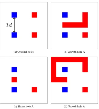
between two distance-dholes needs to be at least 3d. An example of theCNOT braiding evolution [43] between anX-cut qubit and aZ-cut counterpart is illustrated in Fig. 1.8. In the surface code layout, a pair of holes that are 3dapart will serve as a unit cell. Braiding operations can be optimised at the architectural level with regard to the computation

time or lattice area as shown in [135]. At the micro-architectural level, on the other hand,

we need to be able to keep track of the holes’ locations as well as grow and shrink them

by turning off and on the respective syndrome qubits.

1st _{pair of holes}

2nd pair of holes

Time

Fig. 1.7 Braiding diagram of a logicalCNOT gate in surface code with time axis running horizontally.

The code distance is calculated by the intrinsic error rate of the underlying qubit

hardware as well as the threshold of the selected error correction code, as following [86]

εlogical≥C1

C₂εphysical ε_threshold

_⌊d+1

2 ⌋

, (1.8)

whereC1andC2are constants that are code-dependent. For surface code, according to

[46], the values forC₁andC₂are 0.13 and 0.61, respectively. We denote the error rate per logical gate operation asεlogical, which depends on the target success probability

of the algorithm and the number of logical gate operations to complete it. An entire

algorithm success rate ofεalgowill requireεlogical ≈εalgo/Nlogical, whereNlogical is the number of logical gate operations required for the entire computation. The physical error

rateεphysical is the experimental fidelity of the qubits, which is compared against the

(37)

3 d

(a) Original holes (b) Growth hole A

[image:37.595.147.494.113.497.2]

(c) Shrink hole A (d) Growth hole A

Fig. 1.8 LogicalCNOT gate by braiding holes in surface code. The braiding is done by expanding and shrinking a hole. In order to maintain the code distancedthroughout this process, the orginal holes need to be separated by at least 3d.

d. This is the minimum code size that can guarantee the algorithm to be completed with high probability.

From this code distance estimation, we can asymptotically approximate the number

of physical qubits needed and therefore the expected classical resources. Remember

(38)

to estimate the number of physical qubits as follows.

N_physical∝d2×(4×pNlogical)2, (1.9) in which, the number of logical qubitsN_logical is algorithm dependent, and the code distancedis from the previous estimation step.

1.3 Software and Programming

1.3.1 Quantum Programming Languages

A quantum programming language is the means by which quantum algorithms,

sub-routines, or applications can be expressed in a human-comprehensible form yet can be

faithfully and consistently translated into quantum operation sequences which

imple-ments the high-level instructions across various hardware platforms. The abstraction

away from the specific hardware implementation is particularly important at this stage

be-cause we still have a handful of competing platforms which are very different in terms of

low-level operations. For application developers, a consistent and platform-independent

view of quantum computation is the key to innovation and productivity.

Most importantly, the programming language must obey the principles of quantum

computing, namely the no-cloning theorem and the reversibility (unitary) of quantum

operations. On top of that, the language itself needs to be able to cope with emerging

computing models, e.g. the mix of classical and quantum data in a quantum/classical

hybrid programming model.

Early quantum programming language proposals from academic researchers, for

example, QCL (Quantum Computation Language) [208], QGL (Quantum Gate

Lan-guage) [165], Scaffold [3], Chisel-Q [100], or Quipper [60], provide the foundation for

the quantum programming research community. Recently, thanks to the tremendous

interest from industry in quantum computing, we have seen the released of

industry-backed quantum programming languages and development kits/environment. Some of

the most popular are:

(39)

1.4 Quantum Control Engineering 17

• OpenQASM and Quantum Information Software Kit (QISKit) from IBM

• Quil/Forrest from Rigetti

• AQASM from Atos

1.3.2 Quantum Simulation

Since functional quantum computers will not be available anytime soon, we need to be

able to simulate quantum algorithms on conventional computers to validate and debug

those algorithms. The simulation of quantum computers using first principle linear

algebra approach, i.e. matrix-vector multiplication, is strictly memory-bound. The

memory capacity required grows exponentially with the number of qubits involved in

the algorithms.

For reference, one of the largest quantum circuits that have been simulated using

this first principle approach is a 45-qubit simulation, which used 500 terabytes2 of memory on a state-of-the-art supercomputer [81]. There are other various approaches

which could help reduce the memory requirement at the cost of computing time

(space-time trade-offs) or the accuracy of the simulation (e.g. tensor product approximation

methods).

The lack of access to real quantum computing hardware necessitates the use of

quantum simulators to test algorithms and programs. In addition, by deploying multiple

computation models (not just the universal first principle linear algebra approach) on the

simulator back-end, we could provide the best performance outcome for each particular

quantum circuit of interest.

1.4 Quantum Control Engineering

Quantum control engineering, which has been evolving in tandem with quantum

com-puting, plays a vital role in the design and realisation of quantum devices. The ideas

of using feedback control to stabilise naturally-unstable systems are the cornerstone of

classical control theory. Various control techniques can be deployed to autonomously

correct quantum error in the same manner as the conventional QEC schemes.

(40)

Observables, Measurement and Decoherence

• Observables and Measurement

The wavefunction is what defines the probability of finding (measuring) the

particle’s property (e.g. velocity or position) at a certain value.

When a measurement is made, the quantum state is settled (collapsed) into

one of the possibilities. The outcome of the measurement is randomised

according to the wavefunction (quantum state). However, after

measure-ment, the quantum state is completely determined, i.e. we will always get

the same measurement outcome if repeating that measurement.

• Decoherence

Since quantum superposition states collapse if measured, unintended

in-teractions with the surrounding environment can lead to the “leaking” of

quantum information.

In this section, I want to summarise the fundamental concepts of quantum control

and the role it may play in the entire fault-tolerant quantum computing system, or

“stack”. This can be visualised in the diagram in Fig. 1.9 where the quantum control

layer sits just above the hardware qubit implementation. This control layer is supposed

to provide fully-autonomous stability enhancement and error rejection to the underlying

qubit network before any active error correction actions are applied, e.g. measuring

syndrome qubits, decoding for potential errors, etc.

1.4.1 Quantum Noise

The dynamics of quantum states (ψ(t)) are often described in terms of the Schrödinger’s

equation. Foropen quantum systems, the dynamics are described by the Lindblad master equation [19] (Markovian case) which has the following form:

˙

(41)

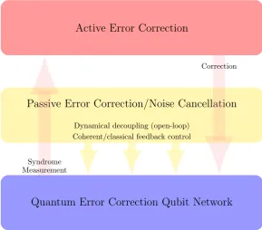
Quantum Error Correction Qubit Network Passive Error Correction/Noise Cancellation

Active Error Correction

Syndrome Measurement

Correction

[image:41.595.173.463.110.364.2]

Coherent/classical feedback control Dynamical decoupling (open-loop)

Fig. 1.9 Combination of passive and active techniques for quantum error correction in which the passive (autonomous) layer improves the stability and/or error rejection to the underlying qubit network before any active error correction actions are applied, e.g. measuring syndrome qubits, decoding for potential errors.

whereρ(t)isdensity matrix,H is the self-energy Hamiltonian operator, and the

super-operatorL is defined as

L∗

L(ρ) =LρL†− 1 2L

†_Lρ

−1

2ρL

†_L_. _(1.11)

The coupling operatorLin equations (1.10) and (1.11) describes the coupling (inter-action) between the quantum system of interest and the external fields (environment/bath).

It is worth noting that we could in principle describe the system + bath as a whole using

the interaction Hamiltonian. This so-called quantum noise model [49, 141], which

describes the overall system in terms of plant and interacting fields (hence coupling

operators), is the foundation of the quantum feedback control field [198, 84, 205].

1.4.2 Quantum Input-Output Model

Emerging engineering problem of extracting information about the dynamical state of

(42)

is another form of the generalised continuous measurement formalism [198]. Front and

centre in this theory is the interaction between the quantum field and system-of-interest

as shown in Fig. 1.10 which in essence has two main effects. Firstly, information about

the system is gained by observing the field output which we will harvest using filtering.

This is the most common mechanism used in any metrology schemes. However, what

distinguishes quantum measurement is the inevitable back-action effect which dictates a

conditional or posterior state of the system consistent which an observed outcome.

Measure after

interaction

filter measurement

signal estimate

before interaction

B(t) Bout(t) System

Y(t) Xˆ(t)

Fig. 1.10 Diagram of a typical quantum filtering set-up.

QHDL (Quantum hardware Description Language) is one of the very first

Computer-Aided-Design (CAD) tools for quantum systems built upon the concept of (S, L, H)

encapsulation. This formulation provides a common thread in the design and verification

flow from schematic capture to an HDL-like description and basic dynamical simulation

with both symbolic and numeric capabilities. Thanks to QHDL, a wide variety of

optical devices can be described in a systematic way that is ready for integration, such

as quantum optical logic gates [107], Set-Reset latch [105], or fully-coherent

error-corrected quantum memory [90].

In the quantum input-output formalism [50], the stochasticevolution of an open Markov quantum system driven by vacuum noise inputs (dA(t)′s) is given by the Hudson-Parthasarathy Quantum Stochastic Differential Equation [79]:

dU(t) = _{−iHdt+ (S₋I)dΛ(t) (1.12)

+

_∑

i

dA†_i(t)L_i₋L†_iSdA_i(t)−1

2L

†

iLidt

) U(t),

in which, the unitary evolutionU(t)is defined on the combined space of the system plant and coupling fields. Any system operator dynamics can be derived from that using

(43)

are referred to as Heisenberg-Langevin equations and completely equivalent to the Schrödinger picture master equation.

This Heisenberg-picture dynamical model can be parametrised conveniently by a

tripleG= (S, L, H), whereHis the internal Hamiltonian,L={L_i_}is a set of coupling operators (e.g. annihilation operators for amplitude damping), andSis a unitary input-to-output scattering matrix (e.g. beam-splitters in quantum optics or quantum point

contacts in solid-state). This parametrisation scheme is often referred to as the SLH

quantum network theory [55, 56].

The network part of this model is what important since from the three parameters

and the given network topology we can compute the equivalent SLH model of the entire

network thanks to the two basic rules as shown in Fig. 1.11.

G1

G2

G1G2

G1 G2

G2CG1

Fig. 1.11 SLH network connections: (left) Concatenation and (right) Cascading.

Mathematically, these two connection rules can be expressed as:

G₂⊞G₁=

 



 S1 0

0 S₂  ,

  L1

L₂ 

,H₁+H₂ 

, (1.13)

G₂◁G₁= (S₂S₁,L₂+S₂L₁,H₁+H₂+Im_{L₂†S₂L₁_}). (1.14) This is the backbone of the QHDL toolbox, whereby network topology (can be in the

form of schematics or Verilog-style inputs as shown in the below example) is processed

symbolically to derive the overall network model. The system dynamics can then be

(44)

Besides the bottom-up approach, we can also perform a top-down decomposition

in the SLH framework by the network synthesis theory [127]. Given an arbitrary SLH

model which may contain a large number of internal dynamical variables (optical modes

or qubits) and inputs/outputs, one can always faithfully identify a suitable collection of

one degree of freedom oscillator components and to connect them serially with proper

Hamiltonian interaction to build up the prescribed system model.

One recent development of the SLH modelling approach is the effort to extend its

application to a wide variety of input states besides the conventional vacuum inputs,

such as thermal field, single-photon and two-photon states [58, 125, 159, 57].

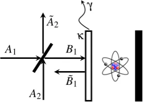
For demonstration purposes, considering a fundamental system of a beam-splitter

(M) and a cavity QED (C) [187] in series as diagrammatically shown in Fig. 1.12.

[image:44.595.202.352.341.447.2]

A₁ A₂ ˜ A2 B₁ ˜ B₁ γ κ

Fig. 1.12 Diagram of beamsplitter in series with cavity QED.

Individually, each component can be described by its corresponding SLH

parame-ters [56]3:

M=

 



 β −α

α β

 ,0,0

 ,

C=

 I,

 

√ κa √

γ σ₋  ,H_c

 ,

H_c=∆fa†a+∆aσ+σ₋+ig(σ+a−σ₋a†),

whereκandγ are the cavity and atomic decay rates, respectively;∆f and∆aare the

detunings;gis the coupling constant between the field and atomic transition.

(45)

-- Structural QHDL generated by gnetlist -- Entity declaration

ENTITY BeamSplitterNetwork IS

PORT (

A1 : in fieldmode;

A2 : in fieldmode;

Vacin : in fieldmode;

B1 : out fieldmode;

B2 : out fieldmode;

Vacout : out fieldmode);

END MachZehnder;

-- Secondary unit

ARCHITECTURE netlist OF BeamSplitterNetwork IS

COMPONENT Beamsplitter

GENERIC (

theta : real := theta_value);

PORT (

In1 : in fieldmode;

In2 : in fieldmode;

Out1 : out fieldmode;

Out2 : out fieldmode);

END COMPONENT ;

COMPONENT SingleSidedJaynesCummings

GENERIC (

kappa : real := kappa_value);

gamma : real := gamma_value);

g : real := g_value);

Delta_a : real := Delta_a_value); Delta_f : real := Delta_f_value);

PORT (

In1 : in fieldmode;

VacIn: in fieldmode;

Out1 : out fieldmode;

UOut : out fieldmode);

END COMPONENT ;

SIGNAL A_1_in : fieldmode;

SIGNAL A_2_in : fieldmode;

SIGNAL A_1_out : fieldmode; SIGNAL A_2_out : fieldmode; SIGNAL B_1_out : fieldmode;

SIGNAL Vac_in : fieldmode;

SIGNAL Vac_out : fieldmode;

BEGIN

-- Architecture statement part

B1 : Beamsplitter PORT MAP (

In1 => A_1_in, In2 => A_2_in, Out1 => A_1_out, Out2 => A_2_out);

C1: SingleSidedJaynesCummings PORT MAP (

In1 => A_1_out, VacIn => Vac_in, Out1 => B_1_out, UOut => Vac_out);

-- Signal assignment part

A_1_in <= A1; A_2_in <= A2; Vac_in <= Vacin; B1 <= B_1_out; B2 <= A_2_out; Vacout <= Vac_out;

END netlist;

(46)

We can easily translate the diagram in Fig. 1.12 into a functional schematic using

appropriate pre-defined components as shown in Fig. 1.14. This can then be rendered

into a QHDL description as listed in Fig. 1.13 which will specify the ports, components,

connections, as well as any user-defined parameters of the system. One can use this to

generate Heisenberg or Schrödinger type dynamical equations to perform simulation or

verification as desired.

In1

In2

Out1

Out2

(₋)

BeamSplitter

In1

Out1

VacIn UOut Cavity

A1

˜

B1

A2

V

ac

In

V

ac

Ou

t

B2=B˜2=A˜2

B1

Fig. 1.14 Sample schematic using QHDL schematic capture tool: A QED cavity is connected in series with a beamsplitter.

1.4.3 Quantum Control

The quantum input-output model, as captured by the (S, L, H) parameter set, bears similarities to the classical control theory. In particular, the output field channels carry

information about the state of the quantum system due to the couplings as described by

theLoperators. This information can be probed by a controller to gain knowledge about the plant, hence can control it to the desired state. This closed plant-controller loop is

the basis of quantum feedback control.

Depending on the nature of the controller used in the feedback loop, quantum control

can be classified into two main categories:

1. Measurement feedback

The output field is measured continuously and the classical measurement signal

(e.g. analog electrical signal or digitised bits) is processed by a classical controller

which could be a Digital Signal Processing (DSP) chip, a Field Programmable

(47)

1.5 Outline 25

Meas. I/V Filter

F

Est.: ˆρ

Target: ρ

+ Quantum Device

Fig. 1.15 Measurement feedback block diagram.

signals based on pre-defined control algorithms. A typical block diagram of a

measurement feedback setup is shown in Fig. 1.15.

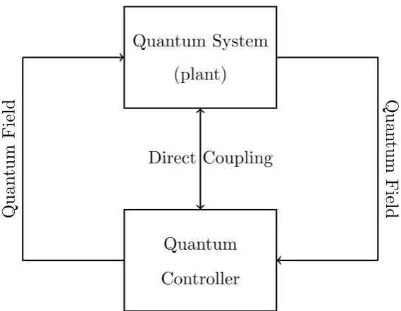
2. Coherent feedback

In coherent feedback control, the output field is fed to another quantum systems

directly as input signals. One quantum system acts as the controller whilst the

other is the plant. No quantum information is “leaked” to the outside world4and thus quantum coherence is preserved in the loop. It is worth noting that besides

field coupling, we could also have direct Hamiltonian coupling between the plant

and controller. This can be described as an interaction Hamiltonian involves

the dynamical variables of both systems. Coherent quantum feedback control is

illustrated in Fig. 1.16.

1.5 Outline

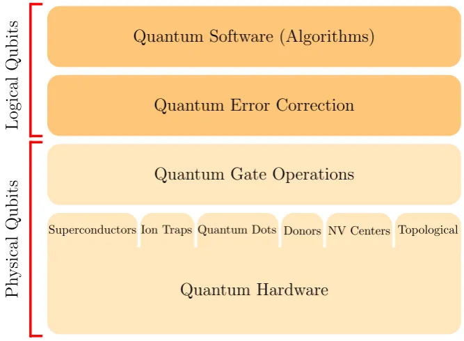
This thesis will study quantum computing at various layers of the quantum “stack” as

depicted in Fig. 1.17, from hardware devices to the error-correction layer as well as

quantum algorithms and applications. More specifically,

• Chapter 2: we investigate the routing scalability of solid-state quantum computers

under 2-dimensional error-correction code, namely the surface code. By applying

the classical electronics know-how regarding interconnect routing to a ubiquitous

2-D qubit array with independent gate control and readout fan-out, we will develop a

concrete procedure for scalability estimation, which is adaptable to a wide range of

(48)

Quantum System

(plant)

Quantum

Controller

Quan

tum

Field

Quan

tum

Field

[image:48.595.134.419.106.327.2]

Direct Coupling

Fig. 1.16 Coherent feedback block diagram.

surface code implementations by adjusting the gate configuration and dimensional

parameters.

• Chapter 3: we look at quantum error correction from a control-engineering centric

standpoint whereby we apply continuous control method to error correction qubit

network. A measurement feedback scheme is used to correct quantum error

continuously in real-time for a surface code 2-dimensional qubit array. The

controller design in this chapter is considered classical since it acquires and processes classical measurement signals to output control signals.

• Chapter 4: we extend the controller design for quantum memory and quantum

error correction into the quantum realm by using techniques of dissipation control

(reservoir engineering) and coherent feedback control. In this chapter,coherent

feedback control technique is used to synthesise perfectly-isolated quantum

infor-mation storage system, namely the decoherence-free subsystem (DFS). Given the

hardware overhead of quantum error correction regarding the number of qubits

depends on the quality of the underlying physical qubits, utilising control

tech-niques to improve qubit stability even before any active error correction operations

are applied as shown in Fig. 1.9 will potentially reduce the amount of overhead

(49)

1.5 Outline 27

Quantum Hardware

Superconductors Ion Traps Quantum Dots Donors NV Centers Topological

Quantum Gate Operations Quantum Error Correction Quantum Software (Algorithms)

Ph

ysical

Qubits

Logical

[image:49.595.152.486.109.354.2]

Qubits

Fig. 1.17 Overall architecture of a universal quantum computer.

• Chapter 5: we discuss the features and the development of a quantum programming

language, namely the Atos Quantum Assembly Language (AQASM) which I was

involved during my research internship at their quantum research lab in Paris.

The new quantum software suite also includes a classical quantum simulator

based on Feynman path integral approach. The simulator was successfully tested

on high-performance computing (HPC) platforms and is complementary to the

linear algebra simulator. A combination of the two is shown to provide the best

performance while not sacrificing the universality of the simulator.

• Chapter 6: we develop a method to simulate quantum open systems based on thequantum controlinput-output formalism on a commercial simulator, namely Microsoft LIQU i_|⟩. A combination of theoretical and practical solutions can provide accurate and consistent simulation results when using a digital gate-based

quantum simulator instead of conventional solver-based simulators.

Lastly, Chapter 7 summarises the content of this thesis with a brief outlook on future

work on quantum control, quantum computing architecture, and quantum programming

language. The follow-up Appendices provides detail proofs and additional information

(50)

1.6 Contributions

The aims of this thesis are

(i) to study a scalability aspect (fanout routing) of fault-tolerant quantum computation

from an engineering perspective (Chapter 2),

(ii) to apply quantum control technology to improve the stability of qubit systems

which are the foundation of the quantum computing hierarchy (Chapter 3 and 4),

and

(iii) to develop practical solutions to enhance quantum software development

(Chap-ter 5) and to bridge the gap between the digital gate-based simulation model and

the dynamical open quantum system model which is the cornerstone of quantum

control theory (Chapter 6).

It represents the author’s attempt to contribute to knowledge through academic

research and industry engagement activities.

Specifically, Chapter 2, 3 and 4 are derived from published works in peer-reviewed

journals or conference proceedings.

Chapter 5 summarises the author’s research results accomplished during an industry

internship with Atos Quantum Lab in Paris, France. Not only was the quantum simulator

successfully commercialised, but a patent has also been granted5 for the simulation method, demonstrating the originality of the work.

Chapter 6 is based on the report that the author produced as an entry to the worldwide

Microsoft Quantum Challenge in which he won the Grand Prize. In this work, the

author has “extended LIQU i_|⟩’s capabilities by supplementing the existing Hamiltonian simulator with an innovative gadget for simulating dissipation. This clever use of

amplitude-damping noise enables a quantum computer to be used to simulate open

quantum systems as well as closed systems, and has important applications in real-world

situations.”6, according to the judges from Microsoft.

5_{France patent No FR3064380, Cyril Allouche and}_{Thien Nguyen}_{, “}_{Procede de Simulation, Sur un}

Ordinateur Classique, D’un Circuit Quantique”, September 28, 2018

(51)

Chapter 2 Solid-state Spin Qubit Control Routing

Every person should have their escape route planned.

Simon Pegg

The need for quantum error correction has a profound implication on the scalability

of future quantum computers. For example, some of the significant problems which

need to be addressed are overhead and complexity in terms of the number of qubits, the

qubit layout design to maintain fault-tolerant properties, and the coordination between

quantum and classical software algorithmically to decode and correct errors as well as

perform the intended quantum algorithm on the quantum computer.

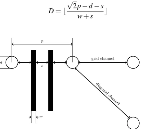
This chapter aims to study the fan-out routing scalability, i.e. the ability to route

planar electrical wires, of surface-code quantum error correction code. To deal with

this question, in this chapter we apply the well-developed routing techniques of modern

semiconductor chip design to solid-state qubit platforms. This chapter proposes a

parametrization scheme which models the qubit layout in terms of the surface gate count

and spacing dimension. The results strongly indicate a bottle-neck which requires novel

architecture designs or technological breakthroughs to provide long-term scalability of

(52)

30 Chapter 2. Solid-state Spin Qubit Control Routing

2.1 Introduction

Building a large-scale quantum computer which can solve classically intractable

prob-lems is a technologically daunting task. With their close connection to highly scalable

classical electronics [72] solid-state spin qubit platforms, such as donor-based qubits [87,

155, 178, 38, 47, 144, 150, 206, 116] and quantum dots [177, 64, 206, 182, 89, 183],

are emerging as promising candidates [10, 40] for scalable quantum computation. On

semiconducting materials, e.g. Si, SiGe, or GaAs, it is possible in principle to fabricate

a large number of interconnecting qubits for quantum information processing. However,

in designing such a large-scale solid-state quantum chip, there is still a gap between the

quantum computer architecture [133, 28, 73, 147, 32, 35, 108, 86, 71] and the physical

qubit device implementation [177, 64, 206]. Architectures necessarily must incorporate

fault-tolerant quantum error correction in order to perform quantum algorithms [122]

at the logical quantum gate level. The physical implementation generally deals with

individual qubits on the basis of physical quantum gate operations, initialisation, and

readout which are the foundation for higher level quantum logical operations. In the

middle ground, quantum computer micro-architectures [86, 180, 71] attempt to bridge

that gap by providing engineering solutions to issues such as classical control, fan-out

interconnects, and chip layout.

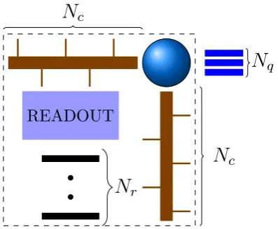
One key advantage of the surface code is its nearest-neighbor interaction scheme

which scales favorably over the concatenation approach. However, this scheme also

re-quires a two-dimensional qubit layout and parallel control. In terms of micro-architecture

considerations, one must account for (a) the spatial/geometrical requirements of a 2D

nearest-neighbor interacting qubit array, and (b) the temporal/control requirements of

parallel/synchronous QEC operations. Broadly, one can identify two approaches. In the

ubiquitous independent control model, each quantum element (qubit, gate, interconnect,

readout) are controlled independently. In principle, this approach has the highest density

of quantum control gates each of which must be carefully characterised and timed to

allow for parallel operation across the qubit array (in a number of steps which does

not depend on the array size). At the other extreme, in the distributed control model

introduced in Hill et al. [71], a high degree of multiplexing allows sufficiently large

Topics in Quantum Computing Architecture