Optotronics: optically inspired electronics

(1)

Thesis by

Ehsan Afshari

In Partial Fulfillment of the Requirements for the Degree of

Doctor of Philosophy

California Institute of Technology Pasadena, California

2006

(2)

c

2006

(3)

To Him who taught me to love

To my mother

(4)

Acknowledgements

During my graduate study at Caltech, I have had the chance to interact with many talented and motivated individuals in multiple disciplines, from all over the world. The most essential lesson that I learned from them, was looking at what everyone else has looked at, and seeing something new. This is the most important key to good research. I would like to express my gratitude to those who have helped me to gain this skill.

First and foremost, I would like to thank my advisor Prof. Ali Hajimiri. He has always been a good friend whom I can count on, and looked after me like an older brother. Despite our many differences, I always enjoy talking to him about all matter of things, from physics to politics. Academically, he has been a fantastic advisor who gave me the freedom to choose my project. He has been extremely patient with me and helped me in all stages of this work. He helped me to choose my carrier path, and fully supported me in pursuing it. He has taught me much and I deeply respect and care for him as a friend and a teacher.

Next, I would like to thank Prof. Jerrold Marsden and Prof. Harish Bhat for their tremendous impact on this work. They convinced me that I am not a mathematician, and helped me realize the power of collaboration. We first started working together in the summer of 2004, when Jerry kindly accepted to help me with my project. He introduced me to Harish, an exceptional mathematician and thinker, without whom this work would not have gone this far. We began a fruitful partnership which holds high hopes for the future. Harish has also been a good friend, whose knowledge and contribution goes well beyond mathematics.

(5)

Sharif-Bakhtiar. He is an extraordinary teacher who could explain the most difficult concepts in a very simple form. He also taught me to be patient in research and showed me the importance of being organized.

Also I would like to thank Prof. Dimitri Psaltis, Prof. David Rutledge, Prof. Sander Weinreb, and Prof. Jerrold Marsden, my candidacy exam committee mem-bers, for their valuable feedbacks. Their technical advice improved the quality of this work, while by sharing their personal experiences they helped clarifying my future carrier options. I would like to thank them for their input and support along the way. Special thanks to my great colleagues and friends who had a substantial influence on my work at Caltech, especially I would like to thank Abbas Komijani for being a great technical and emotional support during the past five years, and Prof. Donhee Ham for helping me to choose the topic of this theses. Additionally, I would like to express my gratitude to all the help and support which was provided by Dr. Behnam Analui and Prof. Hossein Hashemi. Also I would like to thank Prof. Arjang Hassibi, Prof. Hui Wu, Sam Mandegaran, Dr. Saleem Mukhtar, Prof. Jim Buckwalter, Dr. Xiang Guan, Dr. Chris White, Dr. Roberto Aparicio, Edward Keehr, Florian Bohn, Aydin Babakhani, Yu-Jiu Wang, and Hua Wang.

I am also thankful to my friends in Caltech, especially Amir Sadjadpour who tolerated me as a roommate for two years. He has been a true friend, full of love and compassion. I am also grateful to Prof. Babak Hassibi, Mazhar Taghavi, Abbas Nasiraei Moghaddam, Prof. Masoud Sharif, Amir Faraji-Dana, Helia Naemi, Ali Vakili, Arash Yavari, and Shervin Taghavi.

(6)

I have been very lucky to be surrounded by a loving family. I would like to thank Parisa and Erfan for their emotional support and love. As an older sister, Parisa has always been a source of great inspiration. Without a doubt, she is one of the most energetic and goal oriented people that I have ever known. I would also like to thank my in-laws for accepting me as their own. I like to thank Dr. Hossein Azarmnia for being such a great father, full of wisdom and motivation, Mansoureh Sheikhnia for being the coolest mother in-law, full of love and positive energy. I never imagined having a mother in-law like her. I am always eagerly waiting for the weekend when I would meet, and spend time with them. Also I like to thank Morteza for being a great brother. I know that I can always count on him, and I know how much he cares about the family, although he does not make a big show of it. I’d like to thank Mahdi Nilforoushan and Mahboubeh Azarmnia for being great friends to me. This list would not be complete without Daei Reza and Daei Kazem whom I’ve always enjoyed talking to about almost everything, thank you for your kindness and support.

I would like to thank my other half, Monir, for being a great support for me. Without a doubt the most important achievement of my life is finding her, she is everything that I could ask for. In short, she is my best friend in the journey of life. I don’t know how to thank her, Mamnoon Monir! I would also like to thank my mother, Tahereh, for her huge impact in my life. She has been both a mother and father to me. She watched me and looked after me in all stages of my life, and made sacrifices for my advancement that are extraordinary, even for a mother. I would not be who I am today without her unconditional love and support.

(7)

Abstract

Waves are everywhere, from the distribution of cars on a highway to the wave pat-terns in the ocean. Intriguing phenomena in wave propagation, such as Soliton reso-nance, kink-antikink interaction, self-focusing, and Peakon generation can be used in many practical applications leading to novel architectures for signal processing and generation. These E/M based approaches could be particularly useful in the case of Extremely Wide Band (EWB) (DC to more than 100GHz) circuits and systems where the limited transistor cut-off frequency, maximum power efficiency, and breakdown voltage pose serious constraints on the use of conventional circuit techniques.

(8)

(9)

List of Figures

2.1 Waves are everywhere: from music instruments to the surface of ocean and from freeways to Mexican wave in stadiums. . . 7 2.2 a Kelvin-Helmholtz instability rendered visible by clouds in Australia

(source: Wikipedia, the online encyclopedia) . . . 8 2.3 The tidal bore in Turnagain inlet (source: Wikipedia, the online

ency-clopedia) . . . 9 2.4 Soliton on the Scott Russell Aqueduct on the Union Canal (Photograph

by K. Paterson) . . . 11 2.5 Nonlinear interaction of two solitary waves in the coast of California

(Photograph by author) . . . 12 2.6 The one-dimensional atomic chain model . . . 13 2.7 Two examples of electrical wave propagation media: a a 1D LC ladder

and a 2D rectangular LC lattice . . . 17 2.8 A few possible discrete 2D low-pass LC Lattices: each branch is an

inductor and at each node, there is a capacitor to the ground. . . 18 2.9 The lattice can be engineered to achieve desirable transfer function . . 19 2.10 An accumulation mode MOS varactor with its characteristic . . . 19

3.1 1D artificial transmission line . . . 23 3.2 Voltage Vi versus element number i at T = 10 ns for a 1D nonuniform

(15)

3.3 VoltageVi versus element numberi at various times for the (a) uniform

NLTL, with b = 0.5, λ = 0, and (b) nonuniform NLTL, with b = 0.25, λ = 0.02. All other parameters are the same as in the linear case. The input frequency is α = 5 GHz. . . 42 3.4 Voltage Vi versus element numberi for the 1D nonuniform NLTL, with

parameters identical to the previous figure. The outgoing pulse has a larger amplitude and much smaller wavelength than the sinusoidal signal that enters at the left boundary. . . 43

4.1 2D transmission lattice . . . 45 4.2 Keeping Zij constant and defining Tij = n

p

LijCij by the above graph

results in an electric lens. Keeping Tij constant and defining Zij =

p

Lij/Cij by the above graph results in an electric funnel. Note that this

is the precise impedance surface used in the 2D numerical simulations that follow. . . 48 4.3 Voltage Vij as a function of position (i, j) for the 2D nonuniform linear

lattice. . . 58 4.4 Current Iij as a function of position (i, j) for the 2D nonuniform linear

lattice, showing the funneling effect: the signal is stronger in the middle. 58 4.5 Power Pij as a function of position (i, j) for the 2D nonuniform linear

lattice, demonstrating the funneling effect. . . 59 4.6 Efficiency as a function of input frequency for the 2D nonuniform linear

lattice. Note that for an extremely wide range of input frequencies (0 -100 GHz), the lattice focuses ≥60% of the input power. . . 59 4.7 Voltage Vij as a function of position (i, j) for the 2D nonuniform

non-linear lattice. . . 62 4.8 Current Iij as a function of position (i, j) for the 2D nonuniform

(16)

4.9 Power Pij as a function of position (i, j) for the 2D nonuniform

non-linear lattice, demonstrating both the funneling effect and frequency

upconversion. . . 63

4.10 PowerPij as a function of position (i, j) for the 2D nonuniform nonlinear lattice. This shows the same data as Figure (4.9). . . 63

5.1 1D nonuniform linear transmission line . . . 64

5.2 Reflection coefficient as a function of the ratio ω/β, for 2βl = 1. Note that for sufficiently low frequenciesω, more than 15% of the input signal is reflected. . . 75

5.3 Reflection coefficient as a function of ω/β, for 2βl = 10−6.5. Note that the maximum value of the reflection coefficient is less than 10−13 _{so, for} all practical purposes, we have 100% transmission of the input signal. . 76

5.4 1D nonuniform linear transmission line . . . 77

6.1 Three normalized soliton shapes for different values of L and C (a) L=1nH and C= 1nF (b) L=2nH and C=2nF (c) L=4nH and C=4nF . 82 6.2 Dispersion and non-linear effects in the NLTL . . . 83

6.3 Output waveforms of the normal and gradual soliton line . . . 85

6.4 Schematic of the gradually scaled non-linear transmission line . . . 86

6.5 Schematic of an accumulation mode MOS varactor . . . 87

6.6 Capacitance versus voltage for a MOSVAR . . . 87

6.7 How rise and fall time vary within the NLTL . . . 88

6.8 A proposed NLTL for symmetrical edge sharpening . . . 89

6.9 Simple model of a lossy non-linear transmission line with series resisitor 90 6.10 Simple model of a lossy non-linear transmission line with parallel resistor 91 6.11 Measured characteristic of MOSVAR used in the line . . . 92

6.12 Simulated output waveform of the pulse narrowing line using ADS . . 93

(17)

6.14 Chip micro photograph: the middle line is an edge sharpening line and

the other two are pulse narrowing lines. . . 95

6.15 The frequency response of the oscilloscope . . . 96

6.16 The frequency response of the cables, connectors, and probes . . . 97

6.17 Input and output of pulse narrowing line . . . 98

6.18 Response of the measurement setup to an ideal input . . . 98

6.19 Input and output waveforms of the edge sharpening line . . . 99

6.20 Output waveforms of the edge sharpening line with different amplitude verifying the nonlinear behavior of the line . . . 100

7.1 2D square electrical lattice . . . 103

7.2 Basic idea of a funnel . . . 104

7.3 Simulation results of an ideal funnel with 30pH ≤L≤ 150pH and 30fF ≤C ≤ 300fF . . . 105

7.4 Combiner structure . . . 106

7.5 The architecture of power amplifier . . . 106

7.6 Cascode architecture . . . 107

7.7 Maximum stable power gain of a cascode stage vs. a single transistor . 108 7.8 One stand alone distributed power amplifier . . . 108

7.9 Simulated gain of each distributed amplifier . . . 109

7.10 Chip micro photograph . . . 110

7.11 Measurement setup . . . 111

7.12 The power amplifier chip under test . . . 112

7.13 Measured small signal gain of the amplifier . . . 113

7.14 Measured peak output power of the amplifier . . . 113

7.15 Large signal behavior of the amplifier at 85GHz . . . 114

8.1 2-D Nonlinear Transmission Lattice . . . 115

8.2 1-D Nonlinear Transmission Line . . . 116

(18)

8.4 Right boundary of the 2-D electrical lattice, showing the resistive ter-mination. . . 124 8.5 Resonance amplitudeAR and efficiency AR/Aas a function of incoming

amplitude A, for the case of in-phase, equal amplitude incoming waves, showing (1) the robustness of nonlinear combining (AR > 2A) in all

cases; (2) the heightened efficiency for certain input voltages, i.e. two signals of amplitude A= 0.3V combine nonlinearly to produce anAR >

6Aoutput pulse; and (3) the saturation of output amplitudeARfor high

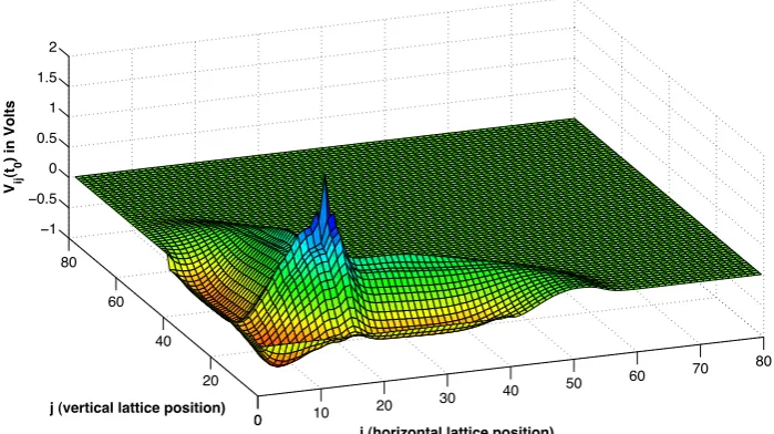
input voltages A. . . 132 8.6 Plot ofVij(t0) for a particular instant of timet0 >0, showing the

gener-ation of a sharp soliton-like nonlinear pulse. The solution shown is for an 80×80 lattice, assuming left- and bottom-boundary input signals (8.14) with equal amplitudes AL = AB = 0.5. The capacitor model is

given by (8.12) with parameters b= 0.5 andVM = 1.9. . . 133

8.7 Resonance amplitude AR as a function of interaction angle θ, for the

case of incoming waves with equal amplitude 0.25V. . . 133 8.8 Voltage Vij(t0) (in Volts) and power Pij(t0) = Vij(t0)Ii+1/2,j(t0) (in

Watts) at a particular instant of time t0 > 0 after three nonlinear in-teractions have occurred, producing a large nonlinear pulse propagating horizontally to the right. . . 134

(19)

9.4 Refraction in a 2-D LC lattice, showing the validity of Snell’s law. The black lines show incident and refracted wave vectors predicted by Snell’s law. Colors correspond to level sets of the voltageVij(t), at a particular

instant of time t > 0. At t = 0, voltage forcing is switched on along the left boundary; resulting waves propagate at an angle, towards the interface at i = 30, where they are refracted, causing a change in the direction and wavelength of the wave. For i < 30, the lattice delay equals τ1, while for i >30, the lattice delay equals τ2. . . 152 9.5 Plane slab showing pure transmission and wavelength expansion in the

20 ≤ i ≤ 70 section. Colors correspond to level sets of the voltage Vij(t), at a particular instant of time t >0. At t= 0, voltage forcing is

switched on along the left boundary; resulting waves propagate to the right, towards the interface ati= 20, where they are refracted, causing a change in wavelength. Ati= 70, the wave encounters a second interface and is refracted again, causing the wavelength to return to its original value. The lattice delay equals τ1 except inside the 20≤i≤70 section, where the delay equals τ2. . . 153 9.6 Total internal reflection. Colors correspond to level sets of the voltage

Vij(t), at a particular instant of time t >0. At t= 0, voltage forcing is

(20)

9.7 Simulation of a uniform 2-D LC lattice showing diffractive effects. The input signal is our choice of forcing function at the left boundary of the lattice, and the output signal is the signal at the right boundary of the lattice. The forcing is sinusoidal and given by (9.25), with ω = 60GHz. Lattice inductances are L= 30pH and lattice capacitances areC = 20fF. 156

9.8 Setup for deriving Green’s function representation of U(P0). . . 157

9.9 Setup for deriving Kirchhoff diffraction integral. . . 159

9.10 Illumination by point source in Kirchhoff diffraction integral. . . 161

9.11 Setup for Sommerfeld Green’s function . . . 162

9.12 Huygens-Fresnel picture showing illumination on a line several wave-lengths away from the thin slit diffraction aperture. . . 164

9.13 Architecture . . . 167

9.14 Results for two different numerical simulations of the 2-D LC lattice showing how diffraction and lensing effects combine to effectively take the spatial 1-D Fourier transform of the input signal. The plots on the left (input signals) correspond to two different choices ofpj in expression (9.33), with ω = 60GHz. Lattice parameters are L = 30pH and C = 20fF, except in a lens-shaped region in the center of the lattice where L is unchanged but C = 60fF. For each input signal, such a lattice was simulated, and the plots on the right show V100,j(t) as a function of vertical section number j, for a particular instant of time t >0. . . 168

9.15 Numerical simulation of the 2-D LC lattice (in black) as compared with our analytical prediction (in blue) and the true Fourier transform (in green) of the input given by (9.34), withω = 60GHz. Lattice parameters are unchanged from Figure 9.14. The black curve shows the numerically computed values of V100,j(t) as a function of vertical section number j, for a particular instant of time t >0. . . 170

(21)

9.17 Simulated outputV100,j(t) at a fixed instant of timet >0, plotted versus

(22)

List of Tables

3.1 Definition of terms . . . 22

7.1 A comparison between this work and other designs . . . 111

8.1 Amplitude AR of the outgoing resonant pulse that forms from two

in-coming sinusoids of amplitude AL and AB. All amplitudes are in Volts. 127

8.2 EfficiencyAR/(AL+AB) (or the ratio of outgoing amplitude to the sum

of incoming amplitudes) as a function of AL and AB. All amplitudes

are in Volts. . . 127 8.3 Output amplitude AR (in Volts) and efficiency AR/A for nonlinear

(23)

Chapter 1 Introduction

“The future of integrated electronics is the future of electronics itself. The advantages

of integration will bring about a proliferation of electronics, pushing this science into

many new areas.” as prophesied G. Moore forty years ago [1]. Today we see the realization of his insight. Not so long ago, a single transistor used to cost a few dollars. Nowadays, for a few dollars we can buy a memory or a microprocessor which has tens of billions transistors on it. It seems that no other field has had such a fast growth.

The continuous development of high performance integrated circuits has led to an explosion in the communication and computation systems. Over the past few years, wireless communication has had an immense growth. Cellular phones are an example of this development. One of the most appealing aspects of wireless networks is that they avoid the high cost of reconfiguring networks: they can be created in just weeks by deploying a small number of base stations, to create high-capacity wireless access systems. They also function well in places where using wires is not an option. The users have the ability to access voice or data while they are mobile, and thousands of subscribers could be connected to a network and share its capacity.

(24)

cell phone subscribers in the US, up from the 34 million users in 1995. More than 25 million households now own laptop computers, and 5.3 million households have wireless Internet access [2].

In this expanding marketplace, integrated circuits technology is chosen based on cost and performance. Technologies such as CMOS, SiGe BiCMOS, InP HBT, GaAs HBT, and GaN HBT can coexist in today’s market due to performance and cost tradeoffs. Most microwave and mm-wave (frequencies beyond 30GHz) applications, such as broadband wireless access or vehicular radars, were only within the realm of compound semiconductors devices. The main problem with compound semiconductor technologies is that they are not cost effective. This is due to their inability to reliably integrate different functions (e.g., digital circuits with large number of transistors) on a single chip. However, unlike compound semiconductors, the major advantage of silicon-based technologies is their ever increasing capacity for integration that enables realization of complex circuits at very low cost. Yet silicon has limited performance at high frequency applications, creating a need for other compounds.

Fortunately, the speed of integrated devices improves as their size shrinks. Device scaling has been the main key to success in the semiconductor industry, and it is applicable for all semiconductor processes including silicon. However, there are at least two impediments to scaling; The first limitation is the huge development cost of a new process, and the second problem is technical complications in very small sized devices. For example, decreasing the size of CMOS devices will result in increasing the gate leakage due to decreasing the gate dielectric thickness and subthershold leakage. This phenomenon increases the idle power of digital gates resulting in the loss of an important advantage of silicon-based technologies. Furthermore, as we reduce transistors sizes, mesoscopic and short channel effects such as hot electron effects, drain induced barrier lowering and mobility degradation transpire. The fundamental limit that we face in scaling the transistors is the gate-dielectric tunneling effect which limits our gate-oxide thickness to a few atoms or approximately 1nm compared to the 3.5nm in production today.

(25)

of building circuit blocks which operate close to the cut-off frequency of the devices or even beyond it. In other words, as faster processes are continuously being de-veloped, we need to develop novel circuit architectures to enhance high frequencies performance.

1.1 Contributions

In this work, we propose novel circuit topologies inspired by commonly used structures in electromagnetics, and more specifically optics. The proposed methodology is based on nonlinear and/or inhomogeneous one-dimensional (1D) transmission lines which we have successfully extended to two-dimensional transmission lattices. The principles behind these designs stem from the mathematical theory of linear and nonlinear wave propagation. By analyzing the models for the transmission lines/lattices, we are able to exploit the large body of theory to design circuits, demonstrating:

• The narrowest reported pulse on silicon (2.5ps),

• The first in-silicon transmission line system capable of sharpening both rising and falling edges of NRZ data by increasing the bandwidth,

• For a single integrated-circuit silicon-based amplifier, the highest achieved cen-ter frequency of operation (85GHz) and the highest achieved power output (120mW) at this frequency,

• Ultra-fast computation systems such as a sub-nanosecond Fourier and Hankel transformers in silicon.

(26)

1.2 Organization

This thesis concentrates on new ways of designing circuits for very high frequency and/or high power applications. Chapter 2 reviews the roots of these design ideas which is the theory of wave propagation in different disciplines. We see that different effects can be studied by wave propagation theory if the natural wavelength is large compared to the microscopic length. Then historical background of soliton pulses is presented. An overview of nonlinear wave propagation in electronics winds up the chapter.

Chapter 3 to 5 cover the theory of wave propagation in one and two dimensional LClattices. they show how to treat the effect of dispersion, nonlinearity, and inhomo-geneity. Several analytical solutions as well as numerical results have been presented. The equations that we consider are mostly the model equations for the circuits shown in chapter 6 and chapter 7. The link between these model equations and well-known equations such as KdV and nonlinear Schr¨odinger equation is studied.

Chapters 6 and chapter 7 introduce the application of these theories. Chapter 6 presents two nonlinear transmission lines. The first one is a soliton line, capable of generating ultra narrow pulses on silicon substrate. Second transmission line can sharpen both rising and falling edges of NRZ data by increasing the bandwidth. The design and measurement of these lines is covered. Chapter 7 shows the application of 2D transmission lattices in broadband power combining. this chapter is wrapped up with simulation and measurement results of a power amplifier fabricated in silicon.

(27)

effects of unequal input amplitudes, out-of-phase input signals, multiple collisions, and non-sinusoidal inputs are considered.

(28)

Chapter 2 Wave Propagation

Waves are everywhere; from the distribution of cars on a highway [3] to the formation of clouds in sky [4], most waves are disturbances that propagate through a medium, often transferring energy. By propagating, waves transfer energy from one point to another, with little or no permanent displacement of the particles of the medium. In other words, relative to the total mass of the medium, there is little or no associated mass transport. Usually waves are oscillations around some fixed positions in a given medium. Figure 2.1 shows few examples of wave phenomenon.

All waves, longitudinal or transverse, electric or elastic, linear or nonlinear, have certain similar behavior in common. The model of wave propagation in a dispersive medium developed by Lord Kelvin, has been successfully used for different types of waves. One can model and explain various phenomena by applying wave propaga-tion theory. As this work focuses more on nonlinear waves and their characteristics, we present the following examples to illustrate this approach. There are excellent references on linear wave phenomena, such as [5][6][7].

2.1 Nonlinear Phenomena

(29)

Figure 2.1: Waves are everywhere: from music instruments to the surface of ocean and from freeways to Mexican wave in stadiums.

the air. This is the well-known Kelvin-Helmholtz instability which results from two adjacent shears of fluids traveling with different velocity. Interestingly, this instability is a function of relative velocity of the shears and it is independent of the density of the fluids. A non-zero curvature will lead to a slight centrifugal force which can cause the flow of one fluid around the other. This effect leads to a change in pressure, which amplifies the ripple. The most familiar example of such a behavior is wind blowing over calm water. Tiny dimples in the smooth surface will quickly be amplified to small waves and finally to frothing white-caps. Referring back to the corn field, if the stalk bending is more than a threshold, the stalk will break resulting in a permanent finger print of the wave over the field. One way to control Kelvin-Helmholtz instabilities is to introduce perpendicular periodicities; that means we could save corns by adding periodic trees perpendicular to the direction of the wind [8].

(30)

a class of clouds called Herringbone clouds. Figure 2.2 shows a good example of such clouds before it diffuses.

Figure 2.2: a Kelvin-Helmholtz instability rendered visible by clouds in Australia (source: Wikipedia, the online encyclopedia)

Yet another place that we have experienced nonlinear effects is car traffic. Whitham [3] was first who modeled car traffic using fluid mechanics and explained the effect of traffic lights, condition of the road, and street junctions with the propagation of shock waves. This approach had led to a breakthrough in studying and controlling the car traffic. [9][10][11][12].

A tidal bore is a remarkable member of the class of the nonlinear waves. It occurs in shallow rivers with a mild slopping riverbed and a broad funnel shaped estuary. The tide forms a wave that travels up in such a river or narrow bay, against the direction of the current [13][14]. For a tidal bore to be formed, a large tidal range -typically more than six meters between high and low water- is necessary. Because of these conditions, bores occur in relatively few locations worldwide. Figure 2.3 shows an example of this fascinating wave.

(31)

Figure 2.3: The tidal bore in Turnagain inlet (source: Wikipedia, the online encyclo-pedia)

and mis its effective mass to take into account the periodicity of the lattice in which the electrons transfer in. If the above parameters are constant, we will end up with Ohm’s law which is a linear relationship between current density and electrical field. However, for large values of electrical field, the electron might be excited to a higher band where the effective mass of the electron may change, due to different relationship between energy and wave number in the new band. For some materials, e.g., GaAs, the effective mass of electron at the new band is larger, resulting in a decrease of J with increasingE. In such a case, the differential resistance is negative and it results in an instability mechanism that leads to propagation of nonlinear stable pulses known as Gunn domains [15]. This phenomenon provide the basic idea for many oscillators [16].

(32)

the earliest ideas on how physical and mathematical processes and constraints affect biological growth were written by D’Arcy Wentworth Thompson [17] and Alan Turing [18]. They showed that a homogenous mixture of chemicals could lead to periodic time variation in the concentration of a particular chemical or to an inhomogeneous spatial separation of chemicals. Also Turing demonstrated that nonlinear chemical reactions together with diffusion could lead to a spatial separation of the chemicals. Later experiments showed that a homogenous mixture of certain chemicals could result in spatial color pattern. All of these effects can be explained in terms of nonlinear wave propagation in time and space.

Conclusion. The message of these wide range of examples is that we could effec-tively study different effects by wave propagation theory if the natural wavelength is large compared to the microscopic length.

2.1.1 Soliton

Perhaps soliton is the most famous nonlinear wave. Soliton is a self-reinforcing soli-tary wave caused by a delicate balance between nonlinear and dispersive effects in the medium. It is not easy to define precisely what a soliton is unless we get into substantial mathematics. Drazin and Johnson [19] describe solitons as solutions of nonlinear differential equations which

1. represent waves of permanent form;

2. are localized, so that they decay or approach a constant at infinity;

3. can interact strongly with other solitons, but they emerge from the collision unchanged apart from a phase shift, so they act somewhat similar to particles.

(33)

Figure 2.4: Soliton on the Scott Russell Aqueduct on the Union Canal (Photograph by K. Paterson)

a well-defined heap of water that continued its course along the channel apparently without change of form or diminution of speed”. He pursued the wave on horseback for more than a mile before returning home to reconstruct it in a water tank. Figure 2.4 shows where he observed soliton and a successful attempt to recreate it. After this discovery, soliton has become important subject of research in diverse fields of physics and engineering. Solitons also occur in other media such as:

• The flow of heat in solids is related to the propagation of solitons. The rela-tionship between soliton amplitude, velocity, and width has been verified. At the microscopic level, usually we deal with phonons. There are number of in-teresting phenomena that can be explained by this point of view. For example we could study phonon-phonon interaction which is essential for understanding thermal conductivity. Fermi, Ulam, and Pasta [21] numerically showed that phonons don’t come to thermal equilibrium, but rather they have nearly pe-riodic variations. Ten years later Zabusky and Kruskal [22] showed that this is correct and it can be explained in terms of solitons. We will discuss this remarkable discovery in the section 2.2.

(34)

chains. He studied chemical changes which leads to the transfer of adenosine triphosphate (ATP) in α-helical protein chains with the idea of soliton propa-gation. Here the dispersion caused by the resonance interaction of intrapeptide dipole vibrations amide-I and nonlinearity caused by the connection of these vibrations with local displacement of equilibrium positions of peptide groups.

• In 1973, Akira Hasegawa [24] of Bell Labs was the first to suggest that solitons could exist in optical fibers, due to a balance between self-phase modulation [25] and anomalous dispersion [26]. He also proposed the idea of a soliton-based transmission system to increase performance of optical telecommunications.

Regardless of their medium, solitary waves show very intriguing properties, for example in a 2D medium, under certain conditions, two solitons can combine in a nonlinear fashion meaning that they combine to a single outgoing wave with peak amplitudegreater than the sum of the incoming waves’ amplitudes. Figure 2.5 shows an example of this phenomenon on the coast of California.

Figure 2.5: Nonlinear interaction of two solitary waves in the coast of California (Photograph by author)

(35)

2.2 Wave Propagation in Periodic Structures

The first work on wave propagation in periodic structures was that of Newton [27] in his effort to derive a formula for the velocity of sound. He modeled the propagation of sound in the air by propagation of an elastic wave along a lattice of masses and springs. The lattice consists of equispaced equal masses, m, that attract each other with elastic force with constant e as shown in figure 2.6.

m m m m m

d

Figure 2.6: The one-dimensional atomic chain model

He obtained a closed form expression for the velocity of sound:

V =d r

e

m =

s ed

ρ (2.1)

where d is the spacing of masses and ρ is density. To verify this model, he used the density of air and isothermal bulk modulus of air as ed. This computed result was smaller than experimental value and hence the model did not match with reality. In 1822 Laplace noticed that expansions and condensations associated with sound waves occur adiabatically and hence adiabatic elastic constant should be used instead of the isothermal value. With this correction the model matched experiments. After this initial work, number of scientists have looked into various kinds of wave propagation in periodic structures. For a complete historical background see [33].

2.2.1 Fermi-Pasta-Ulam Experiment: Birth of Soliton

(36)

For small displacements, the interactions among particles are harmonic and there-fore the equations of motion of particles can be decoupled and the dynamics of the lattice can be described by superposition of mutually independent normal modes. Because these normal modes are independent, if a normal mode is excited, its energy is not transferred to other modes. As a result, a lattice with harmonic oscillations is called nonergodic: it never reaches the thermal equilibrium.

What would happen if we add nonlinearity to the equation? Debye [28] and Peierls [29] suggested that in this case, the normal modes will interact and the energy transfers from one mode to others. Consequently, after many iterations, the system would exhibit ’thermalization’ that is an ergodic behavior in which the influence of the initial modes of vibration fades in importance and the system becomes random, with all modes excited almost equally. In 1955, Fermi, Pasta, Ulam attempted to verify this assumption with one of the first dynamics calculations performed on a computer. They assumed a quadratic nonlinearity and surprisingly they realized that the system does not approach energy equilibrium, that is, the energy in one mode does not spread to the rest. Instead the energy almost periodically returned to the original mode.

(37)

shifts associated with soliton collisions.

In 1967 Gardner [31] showed that if the initial condition is localized, we can find the analytical solution of the KdV equation through inverse scattering method. One year later, Miura [32] developed a method of generating an infinite sequence of constants of motion associated with the KdV equation. This was another explanation of why solitons have their structural stability.

At the end of this section, let us note that the classical work of Brillouin [33] on crystal lattices makes explicit the analogy between crystal lattices, mass-spring models, and LC lattices in one, two, and three spatial dimensions. Brillouin’s primary focus in this work was the development of band-gap theories for lattices with periodic inhomogeneities.

2.3 Nonlinear Waves in Electronics

2.3.1 Motivation

Recently, there has been growing interest in using silicon-based integrated circuits for broadband, high frequency applications. The high level of integration offered by silicon enables numerous new topologies and architectures for low-cost reliable SoC applications at microwave and millimeter wave bands, such as broadband wireless access (e.g., WiMax), vehicular radars at 24GHz and 77GHz citePfeiffer, short range communications at 24GHz and 60GHz, and ultra narrow pulse generation for UWB radar.

If we attempt to build these high frequency boradband circuits with transistors, we are limited by the highest possible transistor cut-off frequency fT, the maximum

(38)

functionality and portability. Also, existing high frequency circuits typically use ei-ther tuned circuits (e.g., LC tank) or microwave techniques (e.g., transmission lines as impedance transformers). These approaches are inherently narrow band and cannot be used in applications such as ultra wide-band impulse radio and ultra wide-band radar (e.g., ground penetrating radar), pulse sharpening, jitter reduction, or a wide band power amplifier.

The theory of wave propagation in linear and nonlinear media is an attractive candidate to face these challenges. For example the ability of solitons to propagate with small dispersion can be used as an effective means to transmit data, modulated as short pulses over long distances; one example of this is the ultra wide band impulse radio that has gained popularity [34].

Furthermore, another advantage of using electrical medium as the wave propa-gation medium is that it could provide a great platform to demonstrate and verify mathematical and physical theories. For example, a two dimensional LC lattice, shown in the next section, is a perfect medium to observe nonlinear wave propaga-tion phenomena such as formapropaga-tion of solitons, kinks, Kelvin-Helmholtz instability, and nonlinear Schr¨odinger equation. It is also possible to develop new phenomena in electrical circuits which have many applications such as power combining and ultra fast specialized computations.

2.3.2 Electrical Wave Propagation Medium

(39)

Li,j

Li,j+1 Li+1,j

Ci,j Li-1,j

Ci+2,j

Li-1,j+1 Ci,j+1 Li,j+2

Li+1,j+1 Ci+2,j+1 Li+2,j+1

Li+3,j Li+2,j

Li+2,j+2 Li+3,j+1

Li Li+1

Ci Ci+1

Li+2

Figure 2.7: Two examples of electrical wave propagation media: a a 1D LC ladder and a 2D rectangular LC lattice

lattice. For details on how to compute this frequency please see Chapters 4 and 8. It is noteworthy that with today’s state of the art integrated circuit technolo-gies, on a silicon substrate, if we use micro strip lines, as inductors and metal to metal capacitance as capacitors, the minimum possible inductance and capacitance are, approximately, LM = 30 pH and CM = 5 fF. Below these values, the parasitic

inductance and capacitance would be dominant. Using these values, we find that the maximum frequency for plane wave propagation on a 2-D rectangilar silicon trans-mission lattice is fM ≈1.16 THz which is much higher than the cut-off frequency of

actives in the same process.

(40)

capac-LC

c

9 . 1 =

ω

LC

c

8 . 2 =

ω

LC

c

23 . 3 =

ω

Figure 2.8: A few possible discrete 2D low-pass LC Lattices: each branch is an inductor and at each node, there is a capacitor to the ground.

itance, or even the termination of different nodes in order to get the desired transfer function. Figure 2.9 shows an example of this idea where input signal is applied to the left boundary and the output signal is taken from the right boundary.

So a transmission surface could be used to process the input signal. This is poten-tially a very fast computation technique and is very similar to changing ε and µof a medium to change the propagation of an EM wave, or the case of quantum mechanics where changing potential barrier could result in desired scattering parameters.

2.3.2.1 Sources of Nonlinearity

The nonlinear elements could be added to the electrical lattice in order to form electrical nonlinear wave propagation media. The nonlinear elements could be voltage dependant capacitors or current dependant inductors. In this work, we mainly focus on nonlinear capacitors, since it is not easy to fabricate nonlinear inductors in today’s integrated processes.

(41)

x

y

a lattice parameter f(x,y)

Input Signal _{Output Signal}

Figure 2.9: The lattice can be engineered to achieve desirable transfer function

reduction in capacitance is due to poly-silicon depletion [36][37] and short-channel charge quantization [37] effects.

n- Well

n+ n+

p- sub n- Well n+

p- sub

n+

C

V

C

V

Figure 2.10: An accumulation mode MOS varactor with its characteristic

2.3.3 Historical Remarks

Compared to other disciplines like optics or plasma physics there has not been lots of work on nonlinear wave propagation in electrical domain.

(42)

phenomena. Scott’s classical treatise [4] was among the first to treat the physics of transmission lines. Scott showed that the Korteweg-de Vries (KdV) equation describes weakly nonlinear waves in the 1D uniform nonlinear transmission line (NLTL). Later, Nejoh showed that if the nonlinearity is moved from the capacitor parallel to the shunt branch of the line to a capacitor parallel to the series branch, the nonlinear Schr¨odinger (NLS) equation is obtained instead [41].

In 1982, model equations for 1D lines that combine nonuniformity, nonlinearity, and resistive loss have been derived by Pantano [42]. In his work, he showed the Burgers- and KdV-type equations govern propagation of waves in NLTL. He also found solitons with varying characteristics. This was a great step toward modeling the NLTL, but more analytical and numerical results were necessary. In other work by Ikezi, numerics and experiments [43] indicated that a nonuniform NLTL could be used for ”temporal contraction” of pulses. Later, Rodwell [44] used nonlinear capacitors on a GaAs substrate to generate picosecond pulses. He also used NLTL to form shock waves with very fast rising edge.

Also, 1D nonlinear transmission lines have been studied by various groups [45] [46] [43] [47] [48] with a focus on generation of ultrashort, high-power, stable electrical pulses. Finally, Ballantyne [49] used a uniform NLTL and a feedback loop to make a baseband soliton oscillator in electrical domain.

Because of lack of application and higher level of complexity, two dimensional nonlinear LC lattices have received much less attention. Recently, Dinkel [50], as-sumed a uniform, nonlinear 2D lattice and showed that the Kadomtsev-Petviashvili (KP) equation [51] describes weakly nonlinear wave propagation in such lattices.

At the other end of the spectrum, nonuniform linear transmission lines have been extensively used by the microwave community for impedance-matching and filtering. In fact, the idea of a nonuniform linear transmission line goes back to the work of Heaviside in the nineteenth century–see Kaufman’s bibliography [52] for details.

(43)

(44)

Chapter 3 Theory of One-Dimensional

Transmission Line

Before proceeding to the theory of wave propagation in 1D transmission line, we make a few definitions , in table 3.1 that will help categorize the transmission lines under consideration.

In this work, We review one-dimensional transmission line theory with the aim of clarifying the effects of discreteness, nonuniformity, and nonlinearity. Continuum equations that accurately model these effects are derived. The speed and ampli-tude of outgoing signals are analyzed directly from the continuum model. We show numerically that introducing weak nonlinearity causes outgoing pulses to assume a soliton-like shape. In the present work, we do not consider current-dependent induc-tors because of implementation issues.

Definitions:

Linear Capacitors and inductors are constant with respect to changes in voltage.

Nonlinear Capacitors are voltage-dependent and/or inductors are current-dependent.

Uniform Identical capacitors and inductors are used throughout the line.

Nonuniform Different capacitors and inductors are used in different parts of the line.

(45)

Figure 3.1: 1D artificial transmission line

3.1 Uniform Nonlinear 1D Transmission Lines

In this section, we review a few facts about uniform NLTLs and their use for pulse narrowing (Figure 3.1). The nonlinear transmission line we consider, consists of series inductors and nonlinear (voltage dependant) shunt capacitors. At node n in the transmission line, Kirchoff’s laws yield the following coupled system of ODEs:

Vn−Vn+1 =

dφn+1/2

dt (3.1a)

In−1/2−In+1/2 = dQn

dt . (3.1b)

Hereφn+1/2 =`In+1/2 is the magnetic flux through the inductor that is between nodes n andn+ 1, and dQn=c(Vn)dVn is the charge on the varactor at noden. Using this,

(3.1) can be rewritten and combined into

`d dt

" c(Vn)

dVn

dt #

(46)

Starting from this semi-discrete model, we develop a continuum model in the standard way. Write xn as the position of node n along the line; assume that the nodes

are equispaced and that h = xn+1 − xn is small. Then, define V(x, t) such that

V(xn, t) =Vn(t). This means thatVn+1 =V(xn+1) =V(xn+h). We Taylor expand

to fourth-order in h and find that (3.2) is equivalent to

`∂ ∂t

"

c(V)∂V ∂t

#

=h2∂ 2_V ∂x2 +

h4 12

∂4_V

∂x4. (3.3)

Let L = `/h and C(V) = c(V)/h be, respectively, the inductance and capacitance per unit length. Then (3.3) becomes

L∂ ∂t

"

C(V)∂V ∂t

# = ∂

2_V ∂x2 +

h2 12

∂4_V

∂x4. (3.4)

We regard this as a continuum model of the transmission line that retains the effect of discreteness in the fourth-order term.

3.1.1 Discreteness Generates Dispersion

Considering small sinusoidal perturbations about a constant voltage V0, we compute the dispersion relation∗ for (3.4):

ω(k) =kv r

1− h

2 12k

2_, _(3.5)

where v = 1/pLC(V0)). We see that for h > 0, ω(k) depends nonlinearly on k. Wavetrains at different frequencies move at different speeds.

In the applied mathematics/physics literature, one finds authors introducing dis-persion into transmission lines through the use of shunt-arm capacitors [41]. This is unnecessary. Experiments on transmission lines we have described, without

shunt-∗_Here_L_and_C _{are distributed parameters with units of, respectively, inductance per unit length}

and capacitance per unit length—this implies thatv has units of velocity. Meanwhile,khas units

of inverse length here, so the quantity hk is dimensionless, consistent with the h→0 limit of the

(47)

arm capacitors, reveal that dispersive spreading of wavetrains due to the discrete nature of the line is a commonly observed phenomenon. Accurate continuum models of the transmission line we have considered should include this discreteness-induced dispersion. Therefore, we use information about the h = 0 case only if it leads to mathematical insights about the h >0 case, which is what truly concerns us.

3.1.2 Traveling Wave Solutions

Retaininghas a small but non-zero parameter, we search for traveling-wave solutions of (3.4), of the form V(x, t) = f(u) where u = x−νt. Using this ansatz and the varactor model C(V) =C0(1−bV), we obtain the following ODE:

(ν2−ν₀2)f00 = h 2_ν2

0 12 f

(4)₊bν2 2 f

200

, (3.6)

whereν₀−2 =LC0and primes denote differentiation with respect tou. Now integrating twice with respect to u, we obtain

(ν2−ν₀2)f = h 2_ν2

0 12 f

00₊ bν2

2 f

2_{+ ˜}_Au_{+ ˜}_B. _(3.7)

We search for a localized solution, for which f, f0, f00 → 0 as u → ±∞. This forces the constants to be zero: ˜A= ˜B = 0. Now multiplying (3.7) by 2f0, integrating with respect to u, and again setting the constant to zero:

(f0)2 =Af2−Bf3, (3.8) where

A = 12(ν 2₋_ν2

0) h2_ν2

0

and B = 4bν 2 h2_ν2 0 .

The first-order ODE (3.8) can be integrated exactly. Taking the integration constant to be zero, we obtain the single-pulse solution

V(x, t) = 3(ν 2₋_ν2

0) bν2 sech

2 " p

3(ν2₋_ν2 0) ν0h

(x−νt) #

(48)

The sech2 form of this pulse is the same as for the soliton solution of the Korteweg-de Vries (KdV) equation. Indeed, applying the reductive perturbation method to (3.4), we obtain KdV in the unidirectional, small-amplitude limit.

3.1.3 Reduction to KdV

Starting with (3.4) and again modeling the varactors byC(V) = C0(1−bV), introduce a small parameterε 1 and change variables via

s=ε1/2(x−ν0t), T =ε3/2t, (3.10)

with ν₀−2 =LC0. Writing

V(x, t) = V(ε−1/2s+ν0ε−3/2T, ε−3/2T), we find that

∂ ∂x =ε

1/2 ∂

∂s and ∂ ∂t =ε

3/2 ∂ ∂T −ε

1/2_ν 0

∂

∂s. (3.11)

Using the formula for C(V), we rewrite the left-hand side of (3.4):

LC0 ∂ ∂t

(1−bV)∂V ∂t

=ν₀−2 ∂ 2 ∂t2

V − b

2V 2

.

Using this and (3.11), we rewrite (3.4) in terms of the long space and time variables s and T:

ν₀−2

ε3 ∂ 2 ∂T2 −2ε

2_ν 0

∂2

∂T ∂s +εν 2 0

∂2 ∂s2

V − b

2V 2

=ε∂

2_V ∂s2 +

h2 12ε

2∂4V

∂s4 (3.12) Now introducing the formal expansion

(49)

the order ε2 _{terms in (3.12) cancel. Keeping terms to lowest order,} _ε3_{, we find}

ν0 ∂2_V

1 ∂s∂T +

bν2 0 4

∂2_V2 1 ∂s2 +

ν2 0h2 24

∂4_V 1

∂s4 = 0, (3.14)

In what follows, we abuse notation by using V to denote V1. Integrating (3.14) with respect to s yields the KdV equation:

∂V ∂T + bν0 2 V ∂V ∂s +

ν0h2 24

∂3V

∂s3 = 0. (3.15)

The KdV equation has been investigated throughly and many of its properties are well-known, including solution by inverse scattering, complete integrability, and geo-metric structure [8]. Hence we will not pursue these topics here.

3.1.4 Remark 1: Zero-Dispersion Case

If we had a purely continuous transmission line, we would take the h → 0 limit of (3.4) and obtain

L∂ ∂t

"

C(V)∂V ∂t

# = ∂

2_V

∂x2. (3.16)

This equation, which in general yields discontinuous shock solutions, has been studied before[58] and we will not repeat the general analysis. However, note that if we carry out the reductive perturbation method on (3.16), we end up with the h→0 limit of (3.15), which is the inviscid Burgers equation:

∂V ∂T +

bc0 2 V

∂V

∂s = 0. (3.17)

It is well-known [59] that for any choice of initial condition V(x,0), no matter how smooth, the solutionV(x, t) of (3.17) develops discontinuities (shock waves) in finite time. Meanwhile, for large classes of initial data, the KdV equation (3.15) possesses solutions that stay smooth globally in space and time[60].

(50)

function uh₍_{x, t}_{). In the work of Lax and Levermore[61], it was shown that in the}

zero-dispersion h→ 0 limit, the sequence uh(x, t) does not converge to a solution of Burgers’ equation (3.17). Therefore, we conclude that the h > 0 continuum model allows fundamentally different phenomena than the h = 0 model. In the nonlinear regime, we must keep track of discreteness.

3.1.5 Remark 2: Linear Case

Note that if C(V) = C is constant, we arrive at the linear, dispersive wave equation

∂2_V ∂t2 −

1 LC

∂2_V ∂x2 =

h2 12

∂4_V

∂x4. (3.18)

This equation can be solved exactly using Fourier transforms. In fact, we will carry out this procedure for a similar equation in the following section.

3.1.6 Frequency Response

So far we have discussed special solutions of (3.4) and the KdV equation. Our primary concern is the transmission lines for the mixing of EWB signals. The physical setup requires that an incoming signal enter the transmission line at, say, its left boundary. The signal is transformed in a particular way and exits the line at, say, its right boundary.

Various authors have examined the initial-value problem for the KdV equation. It is found that, as t → ∞, the solution of the KdV equation consists of a system of interacting solitons. Therefore, we expect that incoming sinusoidal signals will be reshaped into a series of soliton-like pulses. Suppose we wish to determine the precise frequency response in the nonlinear regime: given an input sinusoid of frequency α, we expect to see solitons of frequency F(α) at the output end of the line. We will address the problem of quantitatively determiningF(α) in future work.

(51)

quarter-plane problem

ut+uux+uxxx = 0 (3.19a)

u(x,0+) = 0 (3.19b)

u(0, t) = g(t) (3.19c)

for the KdV equation is not possible at this time. This includes the frequency response problem for whichg(t) =Asinαt. Inverse scattering methods applied to (3.19) yield information only in the simplest of cases, i.e. wheng(t) is a constant[62]. The problem is that in order to close the evolution equations for the scattering data associated with (3.19), one needs to postulate some functional form for ux(0, t) anduxx(0, t). It does

not appear possible to say a priori what these functions should be.

One approach[63] is to postulate that these functions vanish identically for all t. They obtain approximate closed-form solutions in the case where g(t) is a single square-wave pulse, with g(t) ≡ 0 for t > T. In future work, we will investigate whether this is possible if g(t) is a sinusoidal pulse.

In this work, we attempt an analytical solution of the frequency response problem only in the linear regime. For thenonlinear regime, we discuss special solutions and the solution of the initial-value problem for the underlying model equations, to gain a qualitative understanding of the models. For quantitative information about the general nonlinear, nonuniform frequency response problem, we use direct numerical simulations of the semidiscrete model equations.

3.2 Nonuniform Linear 1D

(52)

as a function of position:

∂L ∂x 6= 0,

∂C ∂x 6= 0.

3.2.1 Linear case

For now, assume that the line is linear:

∂L ∂I = 0,

∂C ∂V = 0.

Then, modifying (3.1), we obtain the exact, semi-discrete model

Vn−Vn+1 =`n+1/2

dIn+1/2

dt (3.20a)

In−1/2−In+1/2 =cn

dVn

dt , (3.20b)

which can be combined into the single second-order equation

`n+1/2(Vn−1−Vn)−`n−1/2(Vn−Vn+1) =cn`n−1/2`n+1/2 d2_V

n

dt2 . (3.21) Let L(x) and C(x) be, respectively, the inductance and capacitance per unit length at the position x along the transmission line. This yields the relations L(x) = `n/h

and C(x) =cn/h, and allows us to expand

`n+1/2 =hL(x+h/2) =h

L+ h 2

dL dx +

h2 8

d2L dx2 +

h3 48

d3L

dx3 +O(h 4₎

`n−1/2 =hL(x−h/2) =h

L− h

2 dL dx +

h2 8

d2_L dx2 −

h3 48

d3_L

dx3 +O(h 4₎

.

Expanding V as before, we retain terms up to fifth-order in h on both sides:

h3(LVxx−VxLx) +h5

1

12LVxxxx+ 1

8LxxVxx− 1

6LxVxxx− 1

24LxxxVx

=h3C

L2−h

2 4(Lx)

2

(53)

where we have used subscripts to denote differentiation. We now assume thatLvaries slowly as a function of space, so that LhLx. Hence our continuum model is:

Vxx−LCVtt =Vx

Lx

L −h 2

1

12Vxxxx− 1 6

Lx

LVxxx

. (3.23)

To be clear, we specify that L : [0,∞) → _R and C : [0,∞) → _R are smooth and positive. The parameter h is a measure of discreteness, which as discussed above, contributes dispersion to the line.

3.2.2 Physical Scenario

We are interested in solving the following signaling problem: the transmission line is dead (no voltage, no current) at t = 0, at which point a sinusoidal voltage source is switched on at the left boundary. We assume that the transmission line is long, and that it is terminated at its (physical) right boundary in such a way that the reflection coefficient there is very small. This assumption means that we may model the transmission line as being semi-infinite.

We formalize this as an initial-boundary-value problem (IBVP). Given a transmis-sion line on the half-open interval [0,∞), we seek a functionV(x, t) : [0,∞)×[0,∞)→

R that solves

LCVtt=Vxx+

h2

12Vxxxx− Lx

L

Vx+

h2 6 Vxxx

(3.24a)

V(x,0) = 0 (3.24b)

Vt(x,0) = 0 (3.24c)

V(0, t) =Asinαt (3.24d)

Vx(0, t) = 0 (3.24e)

(54)

3.2.3 Non-Dimensionalization

Examining the form of problem (3.24), we expect that when Lx = 0 (the uniform

case), it may be possible to find exact traveling wave solutions. Hence we exploit the linearity of (3.24a) and seek solutions when L is a slowly varying function of x.

In order to carry this out, we must first non-dimensionalize the continuum model (3.23). Suppose that the transmission line consists of N sections, each of length h. This gives a total length d = N h. Next, suppose that we are interested in the dynamics of (3.24) on the time scale T. Using the constants d and T, we introduce the rescaled, dimensionless length and time variables

x0 = x

d and t

0

= t

T. (3.25)

We then non-dimensionalize (3.23) by writing it in terms of the variables (3.25):

LCd2

T2 Vt0t0 =Vx0x0 + 1

12N2Vx0x0x0x0− Lx0

L (Vx0 + 1

6N2Vx0x0x0). (3.26) For the purposes of notational convenience, we omit primes from now on.

3.2.4 Exponential Tapering

The general nonuniform problem, with arbitrary L and C, may not be classically solvable in closed-form. Here we consider the exponentially tapering given by

L(x) = Beλx (3.27a)

C(x) = 1 Bν2

0

e−λx (3.27b)

(55)

con-siderably to

ν₀−2d2

T2 Vtt =Vxx+ 1

12N2Vxxxx−λ

Vx+

1 6N2Vxxx

. (3.28)

We will analyze this equation subject to the previously discussed initial/boundary conditions (3.24b-3.24e).

3.2.5 Perturbative Solution

We will find solutions of (3.28) accurate to first order in λ. Let us begin by solving the λ = 0 case. Note that the case λ = 0 arose in our discussion of the uniform problem (see (3.18)).

From the setup of the problem, it is clear that the solution will consist of a wavetrain moving to the right at some finite speed. Hence we try the ansatz

V(x, t) =   

 

f(kx−ωt) x < ω_kt

0 x≥ ω

kt

(3.29)

Substituting this into (3.28) gives

ν₀−2d2 T2 ω

2_f00

(z) =k2f00(z) + 1 12N2k

4_f(4)₍_z₎_,

where z = kx −ωt. Integrating twice with respect to z and setting integration constants to zero gives a second-order ODE, which has the general solution

f(kx−ωt) = ¯Asin N p

12(k2₋_ν−2

0 d2T−2ω2)

k2 (kx−ωt) +ψ

! .

Now imposing the boundary condition (3.24d), we solve for the amplitude and phase: ( ¯A, ψ) = (−A,0). We also obtain the dispersion relation

ω2 =k2ν 2 0T2 2d2 1±

r 1− 1

3 ν₀−2h2

T2 α 2

(56)

Because this is a dispersion relation for a non-dimensionalized equation, ω and k are unitless†, as is the parameter α. For a physical solution, the phase velocity must be positive (ω/k >0), so we raise the above equation to the 1/2 power and discard the negative root. Putting everything together, we have the two fundamental modes

V±(x, t) =

  

 

sinhα _ωk ±x−t

i

x < ω±

k t

0 x≥ ω±

k t.

(3.30a)

ω±

k =

ν0T

√

2d 1± r

1−1

3 ν₀−2h2

T2 α 2

!1/2

. (3.30b)

By linearity of (3.28), the general solution of the λ= 0 equation is the superposition

V =−A1V+−A2V−, (3.31)

where A1+A2 =A. Applying the second boundary condition (3.24e) we have

A1 =

Aω+

ω+₋_ω−, A2 =−

Aω−

ω+₋_ω−. (3.32)

3.2.6 Discussion

Using the dispersion relation (3.30b), we can calculate the cut-off frequency of the line. This is the frequency α for which ω becomes imaginary, which in the case of (3.30b) gives the relation

α2 < 3T 2 lc .

Here we used the definition ν₀−1 =√LC whereL=l/hand C =c/h.

Taking h = 0 in the above formula produces the classical solution to the linear wave equation, with the single right-moving mode

ω0/k=ν0.

†_{The careful reader may verify that, because}_L_and_C _{still represent}_distributed _{inductance and}

capacitance, the number ν2

0 has units of velocity squared, implying that the right-hand side of

(57)

Taking h > 0 in (3.30), we find three effects of discreteness. The first is dispersion: though the phase velocity equals the group velocity of the outgoing signal, viz.

ω±

k =

dω±

dk ,

we see from (3.30b) that both of these velocities are nonlinear functions of α, the frequency of the incoming signal. Second, there are now two right-moving modes, one fast and one slow, corresponding to ω+/k and ω−/k. Finally, discreteness causes a decrease in the maximum speed of the wave train; this follows immediately from ω+/k < ω0/k.

3.2.7 General Case

We examine (3.28) withλ >0. On physical grounds we expect that the voltage grows as a function of distance from its starting pointx= 0. Accordingly, we introduce the ansatz

Vλ(x, t) = exp(c1x)f(z) (3.33) where z =kx−ωt. Inserting (3.33) in (3.28), we obtain

ν₀−2ω2f00 = (c2₁f+ 2c1kf0+k2f00) + h2 12 c

4 1f+ 4c

3 1kf

0

+ 6c2₁k2f00+ 4c1k3f(3)+k4f(4)

−λc1f +kf0+ h2

6 c 3 1f + 3c

2 1kf

0

+ 3c1k2f00+k3f(3)

. (3.34)

Choose c1 =λ/2 to eliminate thef(3) terms exactly. Two of thef0 terms cancel. We further ignore all terms of order λm_, _m_≥_{2, obtaining}

ν₀−2ω2f00=k2f00+ h 2 12k

4_f(4)_,

which is precisely the equation we solved in the λ = 0 case. Hence an approximate solution of (3.28), correct to O(λ2_{), is given by}

(58)

with V defined in (3.30-3.32).

Discussion. The qualitative effect of a small but positive value of λ is now clear. The frequency and speed of propagation for the outgoing signal is unchanged from the λ= 0 case. The only effect we expect to observe is growth of the initial sinusoid as it propagates down the line.

Since it appears from (3.35) that we have produced a voltage that is unbounded in space, we remind the reader that in reality, the transmission line is terminated at its right boundary, say at x=X. So long as the resistive termination is chosen so that the reflection coefficient is nearly zero, we may use (3.35) to predict the waveform at any point x∈[0, X].

Remark. Exact solutions of (3.34) can be obtained computationally. Let us outline the procedure in this case. First, we write the full expression of (3.34) in the form

4 X

i=0

qi+1f(i)(z) = 0, whereq=           

−(λ2/4)−(λ4h2/64) (λ3_h2_/₁₂₎_k

k2−ν₀−2ω2 −(λ2h2/8)k2 0

h2k4/12

           . (3.36)

Here we use the convention thatq= (q1, q2, q3, q4, q5). One way to determine a unique solution is to specify the four initial conditions f(i)(0) where i = 0,1,2,3. We leave it as an exercise to show that the four conditions (3.24b-3.24e) also determine the solution uniquely. Then (3.36) can be solved via the matrix exponential. Let y∈_R4 have coordinates yi = f(i−1) for i = 1,2,3,4. Now write (3.36) as the first-order

system

dy

Optotronics: optically inspired electronics

Ehsan Afshari

Acknowledgements

Abstract

Contents

List of Figures

List of Tables

Chapter 1

Introduction

1.1

Contributions

1.2

Organization

Chapter 2

Wave Propagation

2.1

Nonlinear Phenomena

2.1.1

Soliton

2.2

Wave Propagation in Periodic Structures

2.2.1

Fermi-Pasta-Ulam Experiment: Birth of Soliton

2.3

Nonlinear Waves in Electronics

2.3.1

Motivation

2.3.2

Electrical Wave Propagation Medium

C

V

C

V

2.3.3

Historical Remarks

Chapter 3

Theory of One-Dimensional

Transmission Line

3.1

Uniform Nonlinear 1D Transmission Lines

3.1.1

Discreteness Generates Dispersion

3.1.2

Traveling Wave Solutions

3.1.3

Reduction to KdV

3.1.4

Remark 1: Zero-Dispersion Case

3.1.5

Remark 2: Linear Case

3.1.6

Frequency Response

3.2

Nonuniform Linear 1D

3.2.1

Linear case

3.2.2

Physical Scenario

3.2.3

Non-Dimensionalization

3.2.4

Exponential Tapering

3.2.5

Perturbative Solution

3.2.6

Discussion

3.2.7

General Case