BigNum Math
Implementing Cryptographic Multiple Precision Arithmetic
Tom St Denis Greg Rose
Syngress Publishing, Inc., the author(s), and any person or firm involved in the writing, editing, or production (collectively “Makers”) of this book (“the Work”) do not guarantee or warrant the results to be obtained from the Work.
There is no guarantee of any kind, expressed or implied, regarding the Work or its contents. The Work is sold AS IS and WITHOUT WARRANTY. You may have other legal rights, which vary from state to state.
In no event will Makers be liable to you for damages, including any loss of profits, lost savings, or other incidental or consequential damages arising out from the Work or its contents. Because some states do not allow the exclusion or limitation of liability for consequential or incidental damages, the above limitation may not apply to you.
You should always use reasonable care, including backup and other appropriate precautions, when working with computers, networks, data, and files.
Syngress Media, SyngressR , “Career Advancement Through Skill EnhancementR ,”R “Ask the Author UPDATE,” and “Hack ProofingR ,” are registered trademarks ofR Syngress Publishing, Inc. “‘Syngress: The Definition of a Serious Security LibraryTM”, “Mission CriticalTM,” and “The Only Way to Stop a Hacker is to Think Like OneTM” are trademarks of Syngress Publishing, Inc. Brands and product names mentioned in this book are trademarks or service marks of their respective companies.
KEY SERIAL NUMBER
001 HJIRTCV764 002 PO9873D5FG 003 829KM8NJH2 004 HJ9899923N 005 CVPLQ6WQ23 006 VBP965T5T5 007 HJJJ863WD3E 008 2987GVTWMK 009 629MP5SDJT 010 IMWQ295T6T
PUBLISHED BY Syngress Publishing, Inc. 800 Hingham Street
Rockland, MA 02370
Copyright c2006 by Syngress Publishing, Inc. All rights reserved. Printed in Canada. Except as permitted under the Copyright Act of 1976, no part of this publication may be reproduced or distributed in any form or by any means, or stored in a database or retrieval system, without the prior written permission of the publisher, with the exception that the program listings may be entered, stored, and executed in a computer system, but they may not be reproduced for publication.
Printed in the United States of America 1 2 3 4 5 6 7 8 9 0
ISBN: 1597491128
Publisher: Andrew Williams Page Layout and Art: Tom St Denis Copy Editor: Beth Roberts Cover Designer: Michael Kavish
Distributed by O’Reilly Media, Inc. in the United States and Canada.
Contents
Preface xv
1 Introduction 1
1.1 Multiple Precision Arithmetic . . . 1
1.1.1 What Is Multiple Precision Arithmetic? . . . 1
1.1.2 The Need for Multiple Precision Arithmetic . . . 2
1.1.3 Benefits of Multiple Precision Arithmetic . . . 3
1.2 Purpose of This Text . . . 4
1.3 Discussion and Notation . . . 5
1.3.1 Notation . . . 5
1.3.2 Precision Notation . . . 5
1.3.3 Algorithm Inputs and Outputs . . . 6
1.3.4 Mathematical Expressions . . . 6
1.3.5 Work Effort . . . 7
1.4 Exercises . . . 7
1.5 Introduction to LibTomMath . . . 9
1.5.1 What Is LibTomMath? . . . 9
1.5.2 Goals of LibTomMath . . . 9
1.6 Choice of LibTomMath . . . 10
1.6.1 Code Base . . . 10
1.6.2 API Simplicity . . . 11
1.6.3 Optimizations . . . 11
1.6.4 Portability and Stability . . . 12
1.6.5 Choice . . . 12
2 Getting Started 13
2.1 Library Basics . . . 13
2.2 What Is a Multiple Precision Integer? . . . 14
2.2.1 The mp int Structure . . . 15
2.3 Argument Passing . . . 17
2.4 Return Values . . . 18
2.5 Initialization and Clearing . . . 19
2.5.1 Initializing an mp int . . . 19
2.5.2 Clearing an mp int . . . 22
2.6 Maintenance Algorithms . . . 24
2.6.1 Augmenting an mp int’s Precision . . . 24
2.6.2 Initializing Variable Precision mp ints . . . 27
2.6.3 Multiple Integer Initializations and Clearings . . . 29
2.6.4 Clamping Excess Digits . . . 31
3 Basic Operations 35 3.1 Introduction . . . 35
3.2 Assigning Values to mp int Structures . . . 35
3.2.1 Copying an mp int . . . 35
3.2.2 Creating a Clone . . . 39
3.3 Zeroing an Integer . . . 41
3.4 Sign Manipulation . . . 42
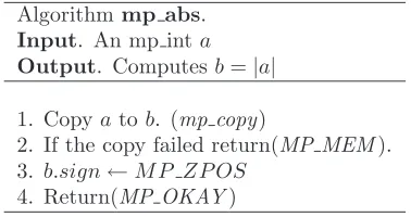
3.4.1 Absolute Value . . . 42
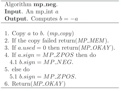
3.4.2 Integer Negation . . . 43
3.5 Small Constants . . . 44
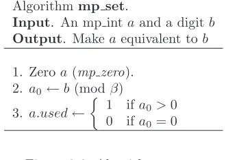
3.5.1 Setting Small Constants . . . 44
3.5.2 Setting Large Constants . . . 46
3.6 Comparisons . . . 47
3.6.1 Unsigned Comparisons . . . 47
3.6.2 Signed Comparisons . . . 50
4 Basic Arithmetic 53 4.1 Introduction . . . 53
4.2 Addition and Subtraction . . . 54
4.2.1 Low Level Addition . . . 54
4.2.2 Low Level Subtraction . . . 59
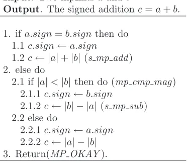
4.2.3 High Level Addition . . . 63
4.3 Bit and Digit Shifting . . . 69
4.3.1 Multiplication by Two . . . 69
4.3.2 Division by Two . . . 72
4.4 Polynomial Basis Operations . . . 75
4.4.1 Multiplication by x. . . 75
4.4.2 Division byx . . . 78
4.5 Powers of Two . . . 81
4.5.1 Multiplication by Power of Two . . . 82
4.5.2 Division by Power of Two . . . 85
4.5.3 Remainder of Division by Power of Two . . . 88
5 Multiplication and Squaring 91 5.1 The Multipliers . . . 91
5.2 Multiplication . . . 92
5.2.1 The Baseline Multiplication . . . 92
5.2.2 Faster Multiplication by the “Comba” Method . . . 97
5.2.3 Even Faster Multiplication . . . 104
5.2.4 Polynomial Basis Multiplication . . . 107
5.2.5 Karatsuba Multiplication . . . 109
5.2.6 Toom-Cook 3-Way Multiplication . . . 116
5.2.7 Signed Multiplication . . . 126
5.3 Squaring . . . 128
5.3.1 The Baseline Squaring Algorithm . . . 129
5.3.2 Faster Squaring by the “Comba” Method . . . 133
5.3.3 Even Faster Squaring . . . 137
5.3.4 Polynomial Basis Squaring . . . 138
5.3.5 Karatsuba Squaring . . . 138
5.3.6 Toom-Cook Squaring . . . 143
5.3.7 High Level Squaring . . . 144
6 Modular Reduction 147 6.1 Basics of Modular Reduction . . . 147
6.2 The Barrett Reduction . . . 148
6.2.1 Fixed Point Arithmetic . . . 148
6.2.2 Choosing a Radix Point . . . 150
6.2.3 Trimming the Quotient . . . 151
6.2.4 Trimming the Residue . . . 152
6.2.6 The Barrett Setup Algorithm . . . 156
6.3 The Montgomery Reduction . . . 158
6.3.1 Digit Based Montgomery Reduction . . . 160
6.3.2 Baseline Montgomery Reduction . . . 162
6.3.3 Faster “Comba” Montgomery Reduction . . . 167
6.3.4 Montgomery Setup . . . 173
6.4 The Diminished Radix Algorithm . . . 175
6.4.1 Choice of Moduli . . . 177
6.4.2 Choice ofk . . . 178
6.4.3 Restricted Diminished Radix Reduction . . . 178
6.4.4 Unrestricted Diminished Radix Reduction . . . 184
6.5 Algorithm Comparison . . . 189
7 Exponentiation 191 7.1 Exponentiation Basics . . . 191
7.1.1 Single Digit Exponentiation . . . 193
7.2 k-ary Exponentiation . . . 195
7.2.1 Optimal Values ofk . . . 196
7.2.2 Sliding Window Exponentiation . . . 197
7.3 Modular Exponentiation . . . 198
7.3.1 Barrett Modular Exponentiation . . . 203
7.4 Quick Power of Two . . . 214
8 Higher Level Algorithms 217 8.1 Integer Division with Remainder . . . 217
8.1.1 Quotient Estimation . . . 219
8.1.2 Normalized Integers . . . 220
8.1.3 Radix-β Division with Remainder . . . 221
8.2 Single Digit Helpers . . . 231
8.2.1 Single Digit Addition and Subtraction . . . 232
8.2.2 Single Digit Multiplication . . . 235
8.2.3 Single Digit Division . . . 237
8.2.4 Single Digit Root Extraction . . . 241
8.3 Random Number Generation . . . 245
8.4 Formatted Representations . . . 247
8.4.1 Reading Radix-n Input . . . 247
9 Number Theoretic Algorithms 255
9.1 Greatest Common Divisor . . . 255
9.1.1 Complete Greatest Common Divisor . . . 258
9.2 Least Common Multiple . . . 263
9.3 Jacobi Symbol Computation . . . 265
9.3.1 Jacobi Symbol . . . 266
9.4 Modular Inverse . . . 271
9.4.1 General Case . . . 273
9.5 Primality Tests . . . 279
9.5.1 Trial Division . . . 279
9.5.2 The Fermat Test . . . 282
9.5.3 The Miller-Rabin Test . . . 284
Bibliography 289
List of Figures
1.1 Typical Data Types for the C Programming Language . . . 2
1.2 Exercise Scoring System . . . 8
2.1 Design Flow of the First Few Original LibTomMath Functions. . . 14
2.2 The mp int Structure . . . 16
2.3 LibTomMath Error Codes . . . 18
2.4 Algorithm mp init . . . 20
2.5 Algorithm mp clear . . . 22
2.6 Algorithm mp grow . . . 25
2.7 Algorithm mp init size . . . 27
2.8 Algorithm mp init multi . . . 29
2.9 Algorithm mp clamp . . . 31
3.1 Algorithm mp copy . . . 36
3.2 Algorithm mp init copy . . . 40
3.3 Algorithm mp zero . . . 41
3.4 Algorithm mp abs . . . 42
3.5 Algorithm mp neg . . . 43
3.6 Algorithm mp set . . . 45
3.7 Algorithm mp set int . . . 46
3.8 Comparison Return Codes . . . 48
3.9 Algorithm mp cmp mag . . . 48
3.10 Algorithm mp cmp . . . 50
4.1 Algorithm s mp add . . . 55
4.2 Algorithm s mp sub . . . 60
4.3 Algorithm mp add . . . 64
4.4 Addition Guide Chart . . . 65
4.5 Algorithm mp sub . . . 67
4.6 Subtraction Guide Chart . . . 67
4.7 Algorithm mp mul 2 . . . 70
4.8 Algorithm mp div 2 . . . 73
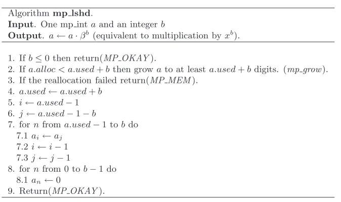
4.9 Algorithm mp lshd . . . 76
4.10 Sliding Window Movement . . . 77
4.11 Algorithm mp rshd . . . 79
4.12 Algorithm mp mul 2d . . . 82
4.13 Algorithm mp div 2d . . . 85
4.14 Algorithm mp mod 2d . . . 88
5.1 Algorithm s mp mul digs . . . 93
5.2 Long-Hand Multiplication Diagram . . . 94
5.3 Comba Multiplication Diagram . . . 98
5.4 Algorithm Comba Fixup . . . 98
5.5 Algorithm fast s mp mul digs . . . 100
5.6 Algorithm fast mult . . . 105
5.7 Asymptotic Running Time of Polynomial Basis Multiplication . . . 108
5.8 Algorithm mp karatsuba mul . . . 111
5.9 Algorithm mp toom mul . . . 118
5.10 Algorithm mp mul . . . 126
5.11 Squaring Optimization Diagram . . . 128
5.12 Algorithm s mp sqr . . . 130
5.13 Algorithm fast s mp sqr . . . 134
5.14 Algorithm mp karatsuba sqr . . . 139
5.15 Algorithm mp sqr . . . 144
6.1 Algorithm mp reduce . . . 153
6.2 Algorithm mp reduce setup . . . 157
6.3 Algorithm Montgomery Reduction . . . 158
6.4 Example of Montgomery Reduction (I) . . . 159
6.5 Algorithm Montgomery Reduction (modified I) . . . 159
6.6 Example of Montgomery Reduction (II) . . . 160
6.7 Algorithm Montgomery Reduction (modified II) . . . 161
6.8 Example of Montgomery Reduction . . . 161
6.9 Algorithm mp montgomery reduce . . . 163
6.11 Algorithm mp montgomery setup . . . 174
6.12 Algorithm Diminished Radix Reduction . . . 176
6.13 Example Diminished Radix Reduction . . . 177
6.14 Algorithm mp dr reduce . . . 179
6.15 Algorithm mp dr setup . . . 182
6.16 Algorithm mp dr is modulus . . . 183
6.17 Algorithm mp reduce 2k . . . 184
6.18 Algorithm mp reduce 2k setup . . . 186
6.19 Algorithm mp reduce is 2k . . . 188
7.1 Left to Right Exponentiation . . . 192
7.2 Example of Left to Right Exponentiation . . . 193
7.3 Algorithm mp expt d . . . 194
7.4 k-ary Exponentiation . . . 196
7.5 Optimal Values ofkfork-ary Exponentiation . . . 197
7.6 Optimal Values ofkfor Sliding Window Exponentiation . . . 197
7.7 Sliding Windowk-ary Exponentiation . . . 198
7.8 Algorithm mp exptmod . . . 199
7.9 Algorithm s mp exptmod . . . 205
7.10 Sliding Window State Diagram . . . 207
7.11 Algorithm mp 2expt . . . 214
8.1 Algorithm Radix-β Integer Division . . . 218
8.2 Algorithm mp div . . . 223
8.3 Algorithm mp add d . . . 232
8.4 Algorithm mp mul d . . . 235
8.5 Algorithm mp div d . . . 238
8.6 Algorithm mp n root . . . 242
8.7 Algorithm mp rand . . . 246
8.8 Lower ASCII Map . . . 248
8.9 Algorithm mp read radix . . . 249
8.10 Algorithm mp toradix . . . 252
8.11 Example of Algorithm mp toradix. . . 253
9.1 Algorithm Greatest Common Divisor (I) . . . 256
9.2 Algorithm Greatest Common Divisor (II) . . . 256
9.3 Algorithm Greatest Common Divisor (III) . . . 257
9.5 Algorithm mp lcm . . . 263
9.6 Algorithm mp jacobi . . . 268
9.7 Algorithm mp invmod . . . 274
9.8 Algorithm mp prime is divisible . . . 280
9.9 Algorithm mp prime fermat . . . 283
Preface
The origins of this book are part of an interesting period of my life. A period that saw me move from a shy and disorganized young adult, into a software developer who has toured various parts of the world, and met countless new friends and colleagues. It all began in December of 2001, nearly five years ago. I started a project that would later become known as LibTomCrypt, and be used by devel-opers throughout industry worldwide.
The LibTomCrypt project was originally started as a way to focus my energies on to something constructive, while also learning new skills. The first year of the project taught me quite a bit about how to organize a product, document and support it and maintain it over time. Around the winter of 2002 I was seeking another project to spread my time with. Realizing that the math performance of LibTomCrypt was lacking, I set out to develop a new math library.
Hence, the LibTomMath project was born. It was originally merely a set of patches against an existing project that quickly grew into a project of its own. Writing the math library from scratch was fundamental to producing a stable and independent product. It also taught me what sort of algorithms are available to do operations such as modular exponentiation. The library became fairly stable and reliable after only a couple of months of development and was immediately put to use.
In the summer of 2003, I was yet again looking for another project to grow into. Realizing that merely implementing the math routines is not enough to truly understand them, I set out to try and explain them myself. In doing so, I eventually mastered the concepts behind the algorithms. This knowledge is what I hope will be passed on to the reader. This text is actually derived from the public domain archives I maintain on my www.libtomcrypt.com Web site.
When I tell people about my LibTom projects (of which there are six) and that I release them as public domain, they are often puzzled. They ask why I
xvi www.syngress.com
did it, and especially why I continue to work on them for free. The best I can explain it is, “Because I can”–which seems odd and perhaps too terse for adult conversation. I often qualify it with “I am able, I am willing,” which perhaps explains it better. I am the first to admit there is nothing that special with what I have done. Perhaps others can see that, too, and then we would have a society to be proud of. My LibTom projects are what I am doing to give back to society in the form of tools and knowledge that can help others in their endeavors.
I started writing this book because it was the most logical task to further my goal of open academia. The LibTomMath source code itself was written to be easy to follow and learn from. There are times, however, where pure C source code does not explain the algorithms properly–hence this book. The book literally starts with the foundation of the library and works itself outward to the more complicated algorithms. The use of both pseudo–code and verbatim source code provides a duality of “theory” and “practice” the computer science students of the world shall appreciate. I never deviate too far from relatively straightforward algebra, and I hope this book can be a valuable learning asset.
This book, and indeed much of the LibTom projects, would not exist in its current form if it were not for a plethora of kind people donating their time, resources, and kind words to help support my work. Writing a text of significant length (along with the source code) is a tiresome and lengthy process. Currently, the LibTom project is five years old, composed of literally thousands of users and over 100,000 lines of source code, TEX, and other material. People like Mads Rassmussen and Greg Rose were there at the beginning to encourage me to work well. It is amazing how timely validation from others can boost morale to continue the project. Definitely, my parents were there for me by providing room and board during the many months of work in 2003.
Both Greg and Mads were invaluable sources of support in the early stages of this project. The initial draft of this text, released in August 2003, was the project of several months of dedicated work. Long hours and still going to school were a constant drain of energy that would not have lasted without support.
Preface xvii
Jim Wigginton, Don Porter, Kevin Kenny, Peter LaDow, Neal Hamilton, David Hulton, Paul Schmidt, Wolfgang Ehrhardt, Johan Lindt, Henrik Goldman, Alex Polushin, Martin Marcel, Brian Gladman, Benjamin Goldberg, Tom Wu, and Pekka Riikonen took their time to contribute ideas, updates, fixes, or encourage-ment throughout the various project developencourage-ment phases. To my many friends whom I have met through the years, I thank you for the good times and the words of encouragement. I hope I honor your kind gestures with this project.
I’d like to thank the editing team at Syngress for poring over 300 pages of text and correcting it in the short span of a single week. I’d like to thank my friends whom I have not mentioned, who were always available for encouragement and a steady supply of fun. I’d like to thank my friends J Harper, Zed Shaw, and Simon Johnson for reviewing the text before submission. I’d like to thank Lance James of the Secure Science Corporation and the entire crew at Elliptic Semiconductor for sponsoring much of my later development time, for sending me to Toorcon, and introducing me to many of the people whom I know today.
Open Source. Open Academia. Open Minds.
xviii www.syngress.com
It’s all because I broke my leg. That just happened to be about the same time Tom asked for someone to review the section of the book about Karatsuba multiplication. I was laid up, alone and immobile, and thought, “Why not?” I vaguely knew what Karatsuba multiplication was, but not really, so I thought I could help, learn, and stop myself from watching daytime cable TV, all at once.
At the time of writing this, I’ve still not met Tom or Mads in meatspace. I’ve been following Tom’s progress since his first splash on the sci.crypt Usenet news-group. I watched him go from a clueless newbie, to the cryptographic equivalent of a reformed smoker, to a real contributor to the field, over a period of about two years. I’ve been impressed with his obvious intelligence, and astounded by his productivity. Of course, he’s young enough to be my own child, so he doesn’t have my problems with staying awake.
When I reviewed that single section of the book, in its earliest form, I was very pleasantly surprised. So I decided to collaborate more fully, and at least review all of it, and perhaps write some bits, too. There’s still a long way to go with it, and I have watched a number of close friends go through the mill of publication, so I think the way to go is longer than Tom thinks it is. Nevertheless, it’s a good effort, and I’m pleased to be involved with it.
Chapter 1
Introduction
1.1
Multiple Precision Arithmetic
1.1.1
What Is Multiple Precision Arithmetic?
When we think of long-hand arithmetic such as addition or multiplication, we rarely consider the fact that we instinctively raise or lower the precision of the numbers we are dealing with. For example, in decimal we almost immediately can reason that 7 times 6 is 42. However, 42 has two digits of precision as opposed to the one digit we started with. Further multiplications of say 3 result in a larger precision result 126. In these few examples we have multiple precisions for the numbers we are working with. Despite the various levels of precision, a single subset1of algorithms can be designed to accommodate them.
By way of comparison, a fixed or single precision operation would lose precision on various operations. For example, in the decimal system with fixed precision 6·7 = 2.
Essentially, at the heart of computer–based multiple precision arithmetic are the same long-hand algorithms taught in schools to manually add, subtract, mul-tiply, and divide.
1With the occasional optimization.
2 www.syngress.com
1.1.2
The Need for Multiple Precision Arithmetic
The most prevalent need for multiple precision arithmetic, often referred to as “bignum” math, is within the implementation of public key cryptography algo-rithms. Algorithms such as RSA [10] and Diffie-Hellman [11] require integers of significant magnitude to resist known cryptanalytic attacks. For example, at the time of this writing a typical RSA modulus would be at least greater than 10309. However, modern programming languages such as ISO C [17] and Java [18] only provide intrinsic support for integers that are relatively small and single precision.
Data Type Range
char −128. . .127
short −32768. . .32767
long −2147483648. . .2147483647
long long −9223372036854775808. . .9223372036854775807
Figure 1.1: Typical Data Types for the C Programming Language
The largest data type guaranteed to be provided by the ISO C programming language2 can only represent values up to 1019 as shown in Figure 1.1. On its own, the C language is insufficient to accommodate the magnitude required for the problem at hand. An RSA modulus of magnitude 1019could be trivially factored3 on the average desktop computer, rendering any protocol based on the algorithm insecure. Multiple precision algorithms solve this problem by extending the range of representable integers while using single precision data types.
Most advancements in fast multiple precision arithmetic stem from the need for faster and more efficient cryptographic primitives. Faster modular reduction and exponentiation algorithms such as Barrett’s reduction algorithm, which have appeared in various cryptographic journals, can render algorithms such as RSA and Diffie-Hellman more efficient. In fact, several major companies such as RSA Security, Certicom, and Entrust have built entire product lines on the implemen-tation and deployment of efficient algorithms.
However, cryptography is not the only field of study that can benefit from fast multiple precision integer routines. Another auxiliary use of multiple precision integers is high precision floating point data types. The basic IEEE [12] standard
2As per the ISO C standard. However, each compiler vendor is allowed to augment the
precision as they see fit.
1.1 Multiple Precision Arithmetic 3
floating point type is made up of an integer mantissaq, an exponente, and a sign bit s. Numbers are given in the form n =q·be· −1s, whereb = 2 is the most
common base for IEEE. Since IEEE floating point is meant to be implemented in hardware, the precision of the mantissa is often fairly small (23, 48, and 64 bits). The mantissa is merely an integer, and a multiple precision integer could be used to create a mantissa of much larger precision than hardware alone can efficiently support. This approach could be useful where scientific applications must minimize the total output error over long calculations.
Yet another use for large integers is within arithmetic on polynomials of large characteristic (i.e.,GF(p)[x] for largep). In fact, the library discussed within this text has already been used to form a polynomial basis library4.
1.1.3
Benefits of Multiple Precision Arithmetic
The benefit of multiple precision representations over single or fixed precision representations is that no precision is lost while representing the result of an operation that requires excess precision. For example, the product of two n-bit integers requires at least 2nbits of precision to be represented faithfully. A multiple precision algorithm would augment the precision of the destination to accommodate the result, while a single precision system would truncate excess bits to maintain a fixed level of precision.
It is possible to implement algorithms that require large integers with fixed precision algorithms. For example, elliptic curve cryptography (ECC) is often implemented on smartcards by fixing the precision of the integers to the maximum size the system will ever need. Such an approach can lead to vastly simpler algorithms that can accommodate the integers required even if the host platform cannot natively accommodate them5. However, as efficient as such an approach may be, the resulting source code is not normally very flexible. It cannot, at run time, accommodate inputs of higher magnitude than the designer anticipated.
Multiple precision algorithms have the most overhead of any style of arith-metic. For the the most part the overhead can be kept to a minimum with careful planning, but overall, it is not well suited for most memory starved platforms. However, multiple precision algorithms do offer the most flexibility in terms of the magnitude of the inputs. That is, the same algorithms based on multiple preci-sion integers can accommodate any reasonable size input without the designer’s
4Seehttp://poly.libtomcrypt.org for more details.
4 www.syngress.com
explicit forethought. This leads to lower cost of ownership for the code, as it only has to be written and tested once.
1.2
Purpose of This Text
The purpose of this text is to instruct the reader regarding how to implement efficient multiple precision algorithms. That is, to explain a limited subset of the core theory behind the algorithms, and the various “housekeeping” elements that are neglected by authors of other texts on the subject. Several texts [1, 2] give considerably detailed explanations of the theoretical aspects of algorithms and often very little information regarding the practical implementation aspects.
In most cases, how an algorithm is explained and how it is actually imple-mented are two very different concepts. For example, the Handbook of Applied Cryptography (HAC), algorithm 14.7 on page 594, gives a relatively simple algo-rithm for performing multiple precision integer addition. However, the description lacks any discussion concerning the fact that the two integer inputs may be of dif-fering magnitudes. As a result, the implementation is not as simple as the text would lead people to believe. Similarly, the division routine (algorithm 14.20, pp. 598) does not discuss how to handle sign or the dividend’s decreasing magnitude in the main loop (step #3).
Both texts also do not discuss several key optimal algorithms required, such as “Comba” and Karatsuba multipliers and fast modular inversion, which we consider practical oversights. These optimal algorithms are vital to achieve any form of useful performance in non–trivial applications.
To solve this problem, the focus of this text is on the practical aspects of implementing a multiple precision integer package. As a case study, the “LibTom-Math”6 package is used to demonstrate algorithms with real implementations7 that have been field tested and work very well. The LibTomMath library is freely available on the Internet for all uses, and this text discusses a very large portion of the inner workings of the library.
The algorithms presented will always include at least one “pseudo-code” de-scription followed by the actual C source code that implements the algorithm. The pseudo-code can be used to implement the same algorithm in other programming languages as the reader sees fit.
1.3 Discussion and Notation 5
This text shall also serve as a walk-through of the creation of multiple precision algorithms from scratch, showing the reader how the algorithms fit together and where to start on various taskings.
1.3
Discussion and Notation
1.3.1
Notation
A multiple precision integer ofn-digits shall be denoted asx= (xn−1, . . . , x1, x0)β
and represent the integerx≡Pn−1
i=0 xiβi. The elements of the arrayxare said to
be the radixβ digits of the integer. For example,x= (1,2,3)10would represent the integer 1·102+ 2·101+ 3·100= 123.
The term “mp int” shall refer to a composite structure that contains the digits of the integer it represents, and auxiliary data required to manipulate the data. These additional members are discussed further in section 2.2.1. For the purposes of this text, a “multiple precision integer” and an “mp int” are assumed synony-mous. When an algorithm is specified to accept an mp int variable, it is assumed the various auxiliary data members are present as well. An expression of the type
variablename.item implies that it should evaluate to the member named “item” of the variable. For example, a string of characters may have a member “length” that would evaluate to the number of characters in the string. If the string a equalshello, then it follows thata.length= 5.
For certain discussions, more generic algorithms are presented to help the reader understand the final algorithm used to solve a given problem. When an algorithm is described as accepting an integer input, it is assumed the input is a plain integer with no additional multiple precision members. That is, algorithms that use integers as opposed to mp ints as inputs do not concern themselves with the housekeeping operations required such as memory management. These algo-rithms will be used to establish the relevant theory that will subsequently be used to describe a multiple precision algorithm to solve the same problem.
1.3.2
Precision Notation
radix-6 www.syngress.com
q factor allows additions and subtractions to proceed without truncation of the carry. Since all modern computers are binary, it is assumed thatqis two.
Within the source code that will be presented for each algorithm, the data typemp digitwill represent a single precision integer type, while the data type mp word will represent a double precision integer type. In several algorithms (notably the Comba routines), temporary results will be stored in arrays of double precision mp words. For the purposes of this text, xj will refer to the j’th digit
of a single precision array, and ˆxj will refer to the j’th digit of a double precision
array. Whenever an expression is to be assigned to a double precision variable, it is assumed that all single precision variables are promoted to double precision during the evaluation. Expressions that are assigned to a single precision variable are truncated to fit within the precision of a single precision data type.
For example, ifβ= 102, a single precision data type may represent a value in the range 0≤x <103, while a double precision data type may represent a value in the range 0≤x < 105. Let a= 23 and b = 49 represent two single precision variables. The single precision product shall be written as c ← a·b, while the double precision product shall be written as ˆc ← a·b. In this particular case, ˆ
c= 1127 and c= 127. The most significant digit of the product would not fit in a single precision data type and as a resultc6= ˆc.
1.3.3
Algorithm Inputs and Outputs
Within the algorithm descriptions all variables are assumed scalars of either single or double precision as indicated. The only exception to this rule is when variables have been indicated to be of type mp int. This distinction is important, as scalars are often used as array indicies and various other counters.
1.3.4
Mathematical Expressions
The ⌊ ⌋ brackets imply an expression truncated to an integer not greater than the expression itself; for example,⌊5.7⌋= 5. Similarly, the⌈ ⌉ brackets imply an expression rounded to an integer not less than the expression itself; for example,
⌈5.1⌉ = 6. Typically, when the / division symbol is used, the intention is to perform an integer division with truncation; for example, 5/2 = 2, which will often be written as ⌊5/2⌋ = 2 for clarity. When an expression is written as a fraction a real value division is implied; for example, 52 = 2.5.
1.4 Exercises 7
||123||= 3 and||79452||= 5.
1.3.5
Work Effort
To measure the efficiency of the specified algorithms, a modified big-Oh notation is used. In this system, all single precision operations are considered to have the same cost8. That is, a single precision addition, multiplication, and division are assumed to take the same time to complete. While this is generally not true in practice, it will simplify the discussions considerably.
Some algorithms have slight advantages over others, which is why some con-stants will not be removed in the notation. For example, a normal baseline mul-tiplication (section 5.2.1) requiresO(n2) work, while a baseline squaring (section 5.3) requires O(n2
+n
2 ) work. In standard big-Oh notation, these would both be said to be equivalent toO(n2). However, in the context of this text, this is not the case, as the magnitude of the inputs will typically be rather small. As a re-sult, small constant factors in the work effort will make an observable difference in algorithm efficiency.
All algorithms presented in this text have a polynomial time work level; that is, of the form O(nk) for n, k ∈ Z+. This will help make useful comparisons in terms of the speed of the algorithms and how various optimizations will help pay off in the long run.
1.4
Exercises
Within the more advanced chapters a section is set aside to give the reader some challenging exercises related to the discussion at hand. These exercises are not designed to be prize–winning problems, but instead to be thought provoking. Wherever possible the problems are forward minded, stating problems that will be answered in subsequent chapters. The reader is encouraged to finish the exercises as they appear to get a better understanding of the subject material.
That being said, the problems are designed to affirm knowledge of a particular subject matter. Students in particular are encouraged to verify they can answer the problems correctly before moving on.
Similar to the exercises as described in [1, pp. ix], these exercises are given a scoring system based on the difficulty of the problem. However, unlike [1], the problems do not get nearly as hard. The scoring of these exercises ranges from
8 www.syngress.com
one (the easiest) to five (the hardest). Figure 1.2 summarizes the scoring system used.
[1] An easy problem that should only take the reader a manner of minutes to solve. Usually does not involve much computer time to solve.
[2] An easy problem that involves a marginal amount of computer time usage. Usually requires a program to be written to solve the problem.
[3] A moderately hard problem that requires a non-trivial amount of work. Usually involves trivial research and development of new theory from the perspective of a student.
[4] A moderately hard problem that involves a non-trivial amount of work and research, the solution to which will demonstrate a higher mastery of the subject matter.
[5] A hard problem that involves concepts that are difficult for a novice to solve. Solutions to these problems will demonstrate a complete mastery of the given subject.
Figure 1.2: Exercise Scoring System
Problems at the first level are meant to be simple questions the reader can answer quickly without programming a solution or devising new theory. These problems are quick tests to see if the material is understood. Problems at the second level are also designed to be easy, but will require a program or algorithm to be implemented to arrive at the answer. These two levels are essentially entry level questions.
Problems at the third level are meant to be a bit more difficult than the first two levels. The answer is often fairly obvious, but arriving at an exacting solution requires some thought and skill. These problems will almost always involve devis-ing a new algorithm or implementdevis-ing a variation of another algorithm previously presented. Readers who can answer these questions will feel comfortable with the concepts behind the topic at hand.
Problems at the fourth level are meant to be similar to those of the level–three questions except they will require additional research to be completed. The reader will most likely not know the answer right away, nor will the text provide the exact details of the answer until a subsequent chapter.
1.5 Introduction to LibTomMath 9
problems have a mastery of the subject matter at hand.
Often problems will be tied together. The purpose of this is to start a chain of thought that will be discussed in future chapters. The reader is encouraged to answer the follow-up problems and try to draw the relevance of problems.
1.5
Introduction to LibTomMath
1.5.1
What Is LibTomMath?
LibTomMath is a free and open source multiple precision integer library written entirely in portable ISO C. Byportableit is meant that the library does not contain any code that is computer platform dependent or otherwise problematic to use on any given platform.
The library has been successfully tested under numerous operating systems, including Unix9, Mac OS, Windows, Linux, Palm OS, and on standalone hard-ware such as the Gameboy Advance. The library is designed to contain enough functionality to be able to develop applications such as public key cryptosystems and still maintain a relatively small footprint.
1.5.2
Goals of LibTomMath
Libraries that obtain the most efficiency are rarely written in a high level program-ming language such as C. However, even though this library is written entirely in ISO C, considerable care has been taken to optimize the algorithm implemen-tations within the library. Specifically, the code has been written to work well with the GNU C Compiler (GCC) on both x86 and ARM processors. Wherever possible, highly efficient algorithms, such as Karatsuba multiplication, sliding win-dow exponentiation, and Montgomery reduction have been provided to make the library more efficient.
Even with the nearly optimal and specialized algorithms that have been in-cluded, the application programing interface (API) has been kept as simple as pos-sible. Often, generic placeholder routines will make use of specialized algorithms automatically without the developer’s specific attention. One such example is the generic multiplication algorithmmp mul(), which will automatically use Toom– Cook, Karatsuba, Comba, or baseline multiplication based on the magnitude of the inputs and the configuration of the library.
10 www.syngress.com
Making LibTomMath as efficient as possible is not the only goal of the LibTom-Math project. Ideally, the library should be source compatible with another pop-ular library, which makes it more attractive for developers to use. In this case, the MPI library was used as an API template for all the basic functions. MPI was chosen because it is another library that fits in the same niche as LibTomMath. Even though LibTomMath uses MPI as the template for the function names and argument passing conventions, it has been written from scratch by Tom St Denis. The project is also meant to act as a learning tool for students, the logic being that no easy-to-follow “bignum” library exists that can be used to teach computer science students how to perform fast and reliable multiple precision integer arith-metic. To this end, the source code has been given quite a few comments and algorithm discussion points.
1.6
Choice of LibTomMath
LibTomMath was chosen as the case study of this text not only because the author of both projects is one and the same, but for more worthy reasons. Other libraries such as GMP [13], MPI [14], LIP [16], and OpenSSL [15] have multiple precision integer arithmetic routines but would not be ideal for this text for reasons that will be explained in the following sub-sections.
1.6.1
Code Base
The LibTomMath code base is all portable ISO C source code. This means that there are no platform–dependent conditional segments of code littered throughout the source. This clean and uncluttered approach to the library means that a developer can more readily discern the true intent of a given section of source code without trying to keep track of what conditional code will be used.
The code base of LibTomMath is well organized. Each function is in its own separate source code file, which allows the reader to find a given function very quickly. On average there are 76 lines of code per source file, which makes the source very easily to follow. By comparison, MPI and LIP are single file projects making code tracing very hard. GMP has many conditional code segments seg-ments that also hinder tracing.
When compiled with GCC for the x86 processor and optimized for speed, the entire library is approximately 100KiB10, which is fairly small compared to GMP
1.6 Choice of LibTomMath 11
(over 250KiB). LibTomMath is slightly larger than MPI (which compiles to about 50KiB), but is also much faster and more complete than MPI.
1.6.2
API Simplicity
LibTomMath is designed after the MPI library and shares the API design. Quite often, programs that use MPI will build with LibTomMath without change. The function names correlate directly to the action they perform. Almost all of the functions share the same parameter passing convention. The learning curve is fairly shallow with the API provided, which is an extremely valuable benefit for the student and developer alike.
The LIP library is an example of a library with an API that is awkward to work with. LIP uses function names that are often “compressed” to illegible shorthand. LibTomMath does not share this characteristic.
The GMP library also does not return error codes. Instead, it uses a POSIX.1 signal system where errors are signaled to the host application. This happens to be the fastest approach, but definitely not the most versatile. In effect, a math error (i.e., invalid input, heap error, etc.) can cause a program to stop functioning, which is definitely undesirable in many situations.
1.6.3
Optimizations
While LibTomMath is certainly not the fastest library (GMP often beats LibTom-Math by a factor of two), it does feature a set of optimal algorithms for tasks such as modular reduction, exponentiation, multiplication, and squaring. GMP and LIP also feature such optimizations, while MPI only uses baseline algorithms with no optimizations. GMP lacks a few of the additional modular reduction optimizations that LibTomMath features11.
LibTomMath is almost always an order of magnitude faster than the MPI library at computationally expensive tasks such as modular exponentiation. In the grand scheme of “bignum” libraries, LibTomMath is faster than the average library and usually slower than the best libraries such as GMP and OpenSSL by only a small factor.
11At the time of this writing, GMP only had Barrett and Montgomery modular reduction
12 www.syngress.com
New Developments
Since the writing of the original manuscript, a new project, TomsFastMath, has been created. It is directly derived from LibTomMath, with a major focus on multiplication, squaring, and reduction performance. It relaxes the portability requirements to use inline assembly for performance. Readers are encouraged to check out this project at http://tfm.libtomcrypt.comto see how far perfor-mance can go with the code in this book.
1.6.4
Portability and Stability
LibTomMath will build “out of the box” on any platform equipped with a modern version of the GNU C Compiler (GCC). This means that without changes the library will build without configuration or setting up any variables. LIP and MPI will build “out of the box” as well but have numerous known bugs. Most notably, the author of MPI has recently stopped working on his library, and LIP has long since been discontinued.
GMP requires a configuration script to run and will not build out of the box. GMP and LibTomMath are still in active development and are very stable across a variety of platforms.
1.6.5
Choice
Chapter 2
Getting Started
2.1
Library Basics
The trick to writing any useful library of source code is to build a solid foundation and work outward from it. First, a problem along with allowable solution param-eters should be identified and analyzed. In this particular case, the inability to accommodate multiple precision integers is the problem. Furthermore, the solu-tion must be written as portable source code that is reasonably efficient across several different computer platforms.
After a foundation is formed, the remainder of the library can be designed and implemented in a hierarchical fashion. That is, to implement the lowest level dependencies first and work toward the most abstract functions last. For example, before implementing a modular exponentiation algorithm, one would implement a modular reduction algorithm. By building outward from a base foundation instead of using a parallel design methodology, you end up with a project that is highly modular. Being highly modular is a desirable property of any project as it often means the resulting product has a small footprint and updates are easy to perform.
Usually, when I start a project I will begin with the header files. I define the data types I think I will need and prototype the initial functions that are not dependent on other functions (within the library). After I implement these base functions, I prototype more dependent functions and implement them. The process repeats until I implement all the functions I require. For example, in the case of LibTomMath, I implemented functions such as mp init() well before
14 www.syngress.com
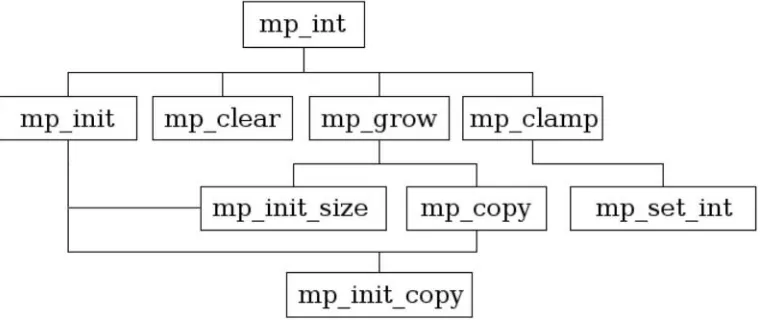
[image:33.504.93.473.182.345.2]I implemented mp mul(), and even further before I implemented mp exptmod(). As an example as to why this design works, note that the Karatsuba and Toom-Cook multipliers were written after the dependent function mp exptmod() was written. Adding the new multiplication algorithms did not require changes to the mp exptmod() function itself and lowered the total cost of ownership and development (so to speak) for new algorithms. This methodology allows new algorithms to be tested in a complete framework with relative ease (Figure 2.1).
Figure 2.1: Design Flow of the First Few Original LibTomMath Functions.
Only after the majority of the functions were in place did I pursue a less hier-archical approach to auditing and optimizing the source code. For example, one day I may audit the multipliers and the next day the polynomial basis functions. It only makes sense to begin the text with the preliminary data types and support algorithms required. This chapter discusses the core algorithms of the library that are the dependents for every other algorithm.
2.2
What Is a Multiple Precision Integer?
2.2 What Is a Multiple Precision Integer? 15
than their precision will allow. The purpose of multiple precision algorithms is to use fixed precision data types to create and manipulate multiple precision integers that may represent values that are very large.
In the decimal system, the largest single digit value is 9. However, by con-catenating digits together, larger numbers may be represented. Newly prepended digits (to the left) are said to be in a different power of ten column. That is, the number 123 can be described as having a 1 in the hundreds column, 2 in the tens column, and 3 in the ones column. Or more formally, 123 = 1·102+ 2·101+ 3·100. Computer–based multiple precision arithmetic is essentially the same concept. Larger integers are represented by adjoining fixed precision computer words with the exception that a different radix is used.
What most people probably do not think about explicitly are the various other attributes that describe a multiple precision integer. For example, the integer 15410 has two immediately obvious properties. First, the integer is positive; that is, the sign of this particular integer is positive as opposed to negative. Second, the integer has three digits in its representation. There is an additional property that the integer possesses that does not concern pencil-and-paper arithmetic. The third property is how many digit placeholders are available to hold the integer.
A visual example of this third property is ensuring there is enough space on the paper to write the integer. For example, if one starts writing a large number too far to the right on a piece of paper, he will have to erase it and move left. Similarly, computer algorithms must maintain strict control over memory usage to ensure that the digits of an integer will not exceed the allowed boundaries. These three properties make up what is known as a multiple precision integer, or mp int for short.
2.2.1
The mp int Structure
16 www.syngress.com
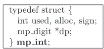
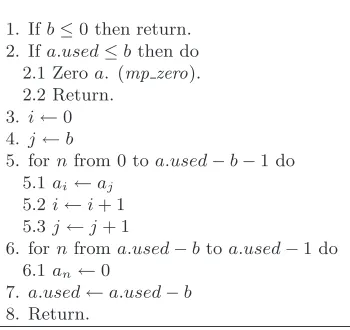
[image:35.504.212.317.73.123.2]typedef struct{ int used, alloc, sign; mp digit *dp; }mp int;
Figure 2.2: The mp int Structure
The mp int structure (Figure 2.2) can be broken down as follows.
• Theused parameter denotes how many digits of the arraydpcontain the digits used to represent a given integer. Theusedcount must be positive (or zero) and may not exceed thealloccount.
• Theallocparameter denotes how many digits are available in the array to use by functions before it has to increase in size. When theusedcount of a result exceeds thealloccount, all the algorithms will automatically increase the size of the array to accommodate the precision of the result.
• The pointerdppoints to a dynamically allocated array of digits that repre-sent the given multiple precision integer. It is padded with (alloc−used) zero digits. The array is maintained in a least significant digit order. As a pencil and paper analogy the array is organized such that the rightmost digits are stored first starting at the location indexed by zero1in the array. For example, ifdp contains{a, b, c, . . .} wheredp0=a,dp1=b,dp2 =c, . . .then it would represent the integera+bβ+cβ2+. . .
• Thesignparameter denotes the sign as either zero/positive (MP ZPOS) or negative (MP NEG).
Valid mp int Structures
Several rules are placed on the state of an mp int structure and are assumed to be followed for reasons of efficiency. The only exceptions are when the structure is passed to initialization functions such as mp init() and mp init copy().
1. The value of allocmay not be less than one. That is, dpalways points to a previously allocated array of digits.
2.3 Argument Passing 17
2. The value ofusedmay not exceedallocand must be greater than or equal to zero.
3. The value of usedimplies the digit at index (used−1) of the dparray is non-zero. That is, leading zero digits in the most significant positions must be trimmed.
(a) Digits in thedparray at and above the usedlocation must be zero.
4. The value of signmust beMP ZPOSif usedis zero; this represents the mp int value of zero.
2.3
Argument Passing
A convention of argument passing must be adopted early in the development of any library. Making the function prototypes consistent will help eliminate many headaches in the future as the library grows to significant complexity. In LibTomMath, the multiple precision integer functions accept parameters from left to right as pointers to mp int structures. That means that the source (input) operands are placed on the left and the destination (output) on the right. Consider the following examples.
mp_mul(&a, &b, &c); /* c = a * b */ mp_add(&a, &b, &a); /* a = a + b */ mp_sqr(&a, &b); /* b = a * a */
The left to right order is a fairly natural way to implement the functions since it lets the developer read aloud the functions and make sense of them. For example, the first function would read “multiply a and b and store in c.”
Certain libraries (LIP by Lenstra for instance ) accept parameters the other way around, to mimic the order of assignment expressions. That is, the destination (output) is on the left and arguments (inputs) are on the right. In truth, it is entirely a matter of preference. In the case of LibTomMath the convention from the MPI library has been adopted.
18 www.syngress.com
variables it must maintain. However, to implement this feature, specific care has to be given to ensure the destination is not modified before the source is fully read.
2.4
Return Values
A well–implemented application, no matter what its purpose, should trap as many runtime errors as possible and return them to the caller. By catching runtime errors a library can be guaranteed to prevent undefined behavior. However, the end developer can still manage to cause a library to crash. For example, by passing an invalid pointer an application may fault by dereferencing memory not owned by the application.
In the case of LibTomMath the only errors that are checked for are related to inappropriate inputs (division by zero for instance) and memory allocation errors. It will not check that the mp int passed to any function is valid, nor will it check pointers for validity. Any function that can cause a runtime error will return an error code as anintdata type with one of the values in Figure 2.3.
Value Meaning
MP OKAY The function was successful
MP VAL One of the input value(s) was invalid MP MEM The function ran out of heap memory
Figure 2.3: LibTomMath Error Codes
When an error is detected within a function, it should free any memory it allocated, often during the initialization of temporary mp ints, and return as soon as possible. The goal is to leave the system in the same state it was when the function was called. Error checking with this style of API is fairly simple.
int err;
if ((err = mp_add(&a, &b, &c)) != MP_OKAY) { printf("Error: %s\n", mp_error_to_string(err)); exit(EXIT_FAILURE);
}
2.5 Initialization and Clearing 19
LibTomMath to force developers to have signal handlers for such cases.
2.5
Initialization and Clearing
The logical starting point when actually writing multiple precision integer func-tions is the initialization and clearing of the mp int structures. These two algo-rithms will be used by the majority of the higher level algoalgo-rithms.
Given the basic mp int structure, an initialization routine must first allocate memory to hold the digits of the integer. Often it is optimal to allocate a suffi-ciently large pre-set number of digits even though the initial integer will represent zero. If only a single digit were allocated, quite a few subsequent reallocations would occur when operations are performed on the integers. There is a trade– off between how many default digits to allocate and how many reallocations are tolerable. Obviously, allocating an excessive amount of digits initially will waste memory and become unmanageable.
If the memory for the digits has been successfully allocated, the rest of the members of the structure must be initialized. Since the initial state of an mp int is to represent the zero integer, the allocated digits must be set to zero, theused count set to zero, andsignset toMP ZPOS.
2.5.1
Initializing an mp int
20 www.syngress.com
Algorithmmp init. Input. An mp inta
Output. Allocate memory and initializeato a known valid mp int state.
1. Allocate memory forMP PRECdigits. 2. If the allocation failed, return(MP MEM) 3. fornfrom 0 toM P P REC−1 do
3.1an←0
4. a.sign←M P ZP OS 5. a.used←0
6. a.alloc←M P P REC 7. Return(MP OKAY)
Figure 2.4: Algorithm mp init
Algorithm mp init. The purpose of this function is to initialize an mp int structure so that the rest of the library can properly manipulate it. It is assumed that the input may not have had any of its members previously initialized, which is certainly a valid assumption if the input resides on the stack.
Before any of the members such assign, used, or alloc are initialized, the memory for the digits is allocated. If this fails, the function returns before setting any of the other members. TheMP PRECname represents a constant2used to dictate the minimum precision of newly initialized mp int integers. Ideally, it is at least equal to the smallest precision number you’ll be working with.
Allocating a block of digits at first instead of a single digit has the benefit of lowering the number of usually slow heap operations later functions will have to perform in the future. If MP PRECis set correctly, the slack memory and the number of heap operations will be trivial.
Once the allocation has been made, the digits have to be set to zero, and the used, sign, and alloc members initialized. This ensures that the mp int will always represent the default state of zero regardless of the original condition of the input.
Remark. This function introduces the idiosyncrasy that all iterative loops, commonly initiated with the “for” keyword, iterate incrementally when the “to” keyword is placed between two expressions. For example, “for afrom bto c do” means that a subsequent expression (or body of expressions) is to be evaluated
2.5 Initialization and Clearing 21
up toc−b times so long asb≤c. In each iteration, the variableais substituted for a new integer that lies inclusively betweenb andc. Ifb > coccurred, the loop would not iterate. By contrast, if the “downto” keyword were used in place of “to,” the loop would iterate decrementally.
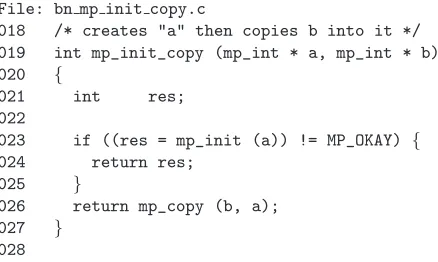
File: bn mp init.c
018 /* init a new mp_int */ 019 int mp_init (mp_int * a) 020 {
021 int i; 022
023 /* allocate memory required and clear it */
024 a->dp = OPT_CAST(mp_digit) XMALLOC (sizeof (mp_digit) * MP_PREC); 025 if (a->dp == NULL) {
026 return MP_MEM;
027 }
028
029 /* set the digits to zero */ 030 for (i = 0; i < MP_PREC; i++) {
031 a->dp[i] = 0;
032 }
033
034 /* set the used to zero, allocated digits to the default precision 035 * and sign to positive */
036 a->used = 0; 037 a->alloc = MP_PREC; 038 a->sign = MP_ZPOS; 039
040 return MP_OKAY; 041 }
042
One immediate observation of this initialization function is that it does not return a pointer to a mp int structure. It is assumed that the caller has already allocated memory for the mp int structure, typically on the application stack. The call to mp init() is used only to initialize the members of the structure to a known default state.
22 www.syngress.com
XMALLOC is not a function but a macro defined in tommath.h. By default, XMALLOC will evaluate to malloc(), which is the C library’s built–in memory allocation routine.
To assure the mp int is in a known state, the digits must be set to zero. On most platforms this could have been accomplished by using calloc() instead of malloc(). However, to correctly initialize an integer type to a given value in a portable fashion, you have to actually assign the value. The for loop (line 30) performs this required operation.
After the memory has been successfully initialized, the remainder of the mem-bers are initialized (lines 34 through 35) to their respective default states. At this point, the algorithm has succeeded and a success code is returned to the calling function. If this function returns MP OKAY, it is safe to assume the mp int structure has been properly initialized and is safe to use with other functions within the library.
2.5.2
Clearing an mp int
When an mp int is no longer required by the application, the memory allocated for its digits must be returned to the application’s memory pool with the mp clear algorithm (Figure 2.5).
Algorithmmp clear. Input. An mp inta
Output. The memory forashall be deallocated.
1. Ifahas been previously freed, then return(MP OKAY). 2. fornfrom 0 toa.used−1 do
2.1an←0
3. Free the memory allocated for the digits ofa. 4. a.used←0
5. a.alloc←0
6. a.sign←M P ZP OS 7. Return(MP OKAY).
Figure 2.5: Algorithm mp clear
acci-2.5 Initialization and Clearing 23
dentally re-uses a cleared structure it is less likely to cause problems. The second goal is to free the allocated memory.
The logic behind the algorithm is extended by marking cleared mp int struc-tures so that subsequent calls to this algorithm will not try to free the memory multiple times. Cleared mp ints are detectable by having a pre-defined invalid digit pointerdpsetting.
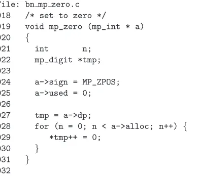
Once an mp int has been cleared, the mp int structure is no longer in a valid state for any other algorithm with the exception of algorithms mp init, mp init copy, mp init size, and mp clear.
File: bn mp clear.c
018 /* clear one (frees) */ 019 void
020 mp_clear (mp_int * a) 021 {
022 int i; 023
024 /* only do anything if a hasn’t been freed previously */ 025 if (a->dp != NULL) {
026 /* first zero the digits */ 027 for (i = 0; i < a->used; i++) {
028 a->dp[i] = 0;
029 }
030
031 /* free ram */ 032 XFREE(a->dp); 033
034 /* reset members to make debugging easier */ 035 a->dp = NULL;
036 a->alloc = a->used = 0; 037 a->sign = MP_ZPOS;
038 }
039 }
040
The algorithm only operates on the mp int if it hasn’t been previously cleared. The if statement (line 25) checks to see if the dp member is not NULL. If the mp int is a valid mp int, thendpcannot beNULL, in which case the if statement will evaluate to true.
24 www.syngress.com
zero to every digit. Similar to mp init(), the digits are assigned zero instead of using block memory operations (such as memset()) since this is more portable.
The digits are deallocated off the heap via the XFREE macro. Similar to XMALLOC, the XFREE macro actually evaluates to a standard C library func-tion; in this case, free(). Since free() only deallocates the memory, the pointer still has to be reset to NULLmanually (line 35).
Now that the digits have been cleared and deallocated, the other members are set to their final values (lines 36 and 37).
2.6
Maintenance Algorithms
The previous sections described how to initialize and clear an mp int structure. To further support operations that are to be performed on mp int structures (such as addition and multiplication), the dependent algorithms must be able to augment the precision of an mp int and initialize mp ints with differing initial conditions.
These algorithms complete the set of low–level algorithms required to work with mp int structures in the higher level algorithms such as addition, multipli-cation, and modular exponentiation.
2.6.1
Augmenting an mp int’s Precision
2.6 Maintenance Algorithms 25
Algorithmmp grow.
Input. An mp intaand an integerb.
Output. ais expanded to accommodatebdigits.
1. ifa.alloc≥b, then return(MP OKAY) 2. u←b(mod M P P REC)
3. v←b+ 2·M P P REC−u
4. Reallocate the array of digitsato sizev
5. If the allocation failed, then return(MP MEM). 6. for n from a.alloc tov−1 do
6.1an←0
7. a.alloc←v
8. Return(MP OKAY)
Figure 2.6: Algorithm mp grow
Algorithm mp grow. It is ideal to prevent reallocations from being per-formed if they are not required (step one). This is useful to prevent mp ints from growing excessively in code that erroneously calls mp grow.
The requested digit count is padded up to the next multiple of MP PREC plus an additionalMP PREC(steps two and three). This helps prevent many trivial reallocations that would grow an mp int by trivially small values.
It is assumed that the reallocation (step four) leaves the lower a.alloc digits of the mp int intact. This is much akin to how the realloc function from the standard C library works. Since the newly allocated digits are assumed to contain undefined values, they are initially set to zero.
File: bn mp grow.c
018 /* grow as required */
019 int mp_grow (mp_int * a, int size) 020 {
021 int i;
022 mp_digit *tmp; 023
024 /* if the alloc size is smaller alloc more ram */ 025 if (a->alloc < size) {
026 /* ensure there are always at least MP_PREC digits extra on top */ 027 size += (MP_PREC * 2) - (size % MP_PREC);
26 www.syngress.com
029 /* reallocate the array a->dp
030 *
031 * We store the return in a temporary variable 032 * in case the operation failed we don’t want 033 * to overwrite the dp member of a.
034 */
035 tmp = OPT_CAST(mp_digit) XREALLOC (a->dp, sizeof (mp_digit) * size); 036 if (tmp == NULL) {
037 /* reallocation failed but "a" is still valid [can be freed] */
038 return MP_MEM;
039 }
040
041 /* reallocation succeeded so set a->dp */ 042 a->dp = tmp;
043
044 /* zero excess digits */
045 i = a->alloc;
046 a->alloc = size;
047 for (; i < a->alloc; i++) {
048 a->dp[i] = 0;
049 }
050 }
051 return MP_OKAY; 052 }
053
A quick optimization is to first determine if a memory reallocation is required at all. The if statement (line 24) checks if the alloc member of the mp int is smaller than the requested digit count. If the count is not larger thanalloc the function skips the reallocation part, thus saving time.
When a reallocation is performed, it is turned into an optimal request to save time in the future. The requested digit count is padded upwards to 2nd multiple of MP PREC larger than alloc (line 25). The XREALLOC function is used to reallocate the memory. As per the other functions, XREALLOC is actually a macro that evaluates to realloc by default. The realloc function leaves the base of the allocation intact, which means the first allocdigits of the mp int are the same as before the reallocation. All that is left is to clear the newly allocated digits and return.
2.6 Maintenance Algorithms 27
releases of the library stored the result of XREALLOC into the mp inta. That would result in a memory leak if XREALLOC ever failed.
2.6.2
Initializing Variable Precision mp ints
Occasionally, the number of digits required will be known in advance of an initial-ization, based on, for example, the size of input mp ints to a given algorithm. The purpose of algorithm mp init size is similar to mp init except that it will allocate
at least a specified number of digits (Function 2.7).
Algorithmmp init size.
Input. An mp intaand the requested number of digitsb.
Output. ais initialized to hold at leastbdigits.
1. u←b(modM P P REC) 2. v←b+ 2·M P P REC−u
3. Allocatevdigits. 4. fornfrom 0 tov−1 do
4.1an←0
5. a.sign←M P ZP OS
6. a.used←0 7. a.alloc←v
8. Return(MP OKAY)
Figure 2.7: Algorithm mp init size
Algorithm mp init size. This algorithm will initialize an mp int structurea like algorithm mp init, with the exception that the number of digits allocated can be controlled by the second input argumentb. The input size is padded upwards so it is a multiple of MP PREC plus an additionalMP PREC digits. This padding is used to prevent trivial allocations from becoming a bottleneck in the rest of the algorithms (Figure 2.7).
Like algorithm mp init, the mp int structure is initialized to a default state representing the integer zero. This particular algorithm is useful if it is known ahead of time the approximate size of the input. If the approximation is correct, no further memory reallocations are required to work with the mp int.
File: bn mp init size.c
28 www.syngress.com
019 int mp_init_size (mp_int * a, int size) 020 {
021 int x; 022
023 /* pad size so there are always extra digits */ 024 size += (MP_PREC * 2) - (size % MP_PREC); 025
026 /* alloc mem */
027 a->dp = OPT_CAST(mp_digit) XMALLOC (sizeof (mp_digit) * size); 028 if (a->dp == NULL) {
029 return MP_MEM;
030 }
031
032 /* set the members */ 033 a->used = 0;
034 a->alloc = size; 035 a->sign = MP_ZPOS; 036
037 /* zero the digits */ 038 for (x = 0; x < size; x++) {
039 a->dp[x] = 0;
040 }
041
042 return MP_OKAY; 043 }
044
The number of digits b requested is padded (line 24) by first augmenting it to the next multiple of MP PRECand then addingMP PRECto the result. If the memory can be successfully allocated, the mp int is placed in a default state representing the integer zero. Otherwise, the error codeMP MEMwill be returned (line 29).
2.6 Maintenance Algorithms 29
2.6.3
Multiple Integer Initializations and Clearings
Occasionally, a function will require a series of mp int data types to be made available simultaneously. The purpose of algorithm mp init multi (Figure 2.8) is to initialize a variable length array of mp int structures in a single statement. It is essentially a shortcut to multiple initializations.
Algorithmmp init multi.
Input. Variable length arrayVk of mp int variables of lengthk.
Output. The array is initialized such that each mp int ofVk is ready to use.
1. for nfrom 0 tok−1 do
1.1. Initialize the mp intVn (mp init)
1.2. If initialization failed then do 1.2.1. forj from 0 tondo
1.2.1.1. Free the mp intVj (mp clear)
1.2.2. Return(MP MEM) 2. Return(MP OKAY)
Figure 2.8: Algorithm mp init multi
Algorithm mp init multi. The algorithm will initialize the array of mp int variables one at a time. If a runtime error has been detected (step 1.2), all of the previously initialized variables are cleared. The goal is an “all or nothing” initialization, which allows for quick recovery from runtime errors (Figure 2.8).
File: bn mp init multi.c 017 #include <stdarg.h> 018
019 int mp_init_multi(mp_int *mp, ...) 020 {
021 mp_err res = MP_OKAY; /* Assume ok until proven otherwise */
022 int n = 0; /* Number of ok inits */
023 mp_int* cur_arg = mp; 024 va_list args;
025
026 va_start(args, mp); /* init args to next argument from caller */ 027 while (cur_arg != NULL) {