Article
A Study of Flowrate Calculation Using ESPRIT Technique
for Ultrasonic Velocity Profiles
Jatuphol Daosaeng
aand Natee Thong-un
b,*Department of Instrumentation and Electronics Engineering, Faculty of Engineering, King Mongkut’s University of Technology North Bangkok, Thailand
E-mail: a[email protected], b[email protected] (Corresponding author)
Abstract. An ultrasonic Velocity Profile (UVP) has been continuously improved for
flowrate measurements. Since the UVP can visualize a flow profile along a cross section of pipelines, it provides a significant advantage over other conventional methods such as differential pressure, turbine, and vortex. Previously, the UVP was realized by means of autocorrelation, fast Fourier transform, and wavelet as the signal-processing method. An Estimation of Signal Parameters via Rotational Invariance Technique (ESPRIT) has been widely used in a field of communication engineering for a high-resolution signal processing. This is the first of utilizing the ESPRIT technique in fluid mechanics for a flowrate computation. To guarantee the proposed idea, the results were compared with a standard electromagnetic flowmeter. Lab experiments were required to demonstrate the accuracy of flowrate measurements.
Keywords: Velocity profiles, flowrate measurement, ESPRIT.
ENGINEERING JOURNAL Volume 23 Issue 2
1.
Introduction
Single phase flow characteristic is more fascination to many researchers and engineers to study a liquid flowrate. Differential pressure flowmeters such as orifice plates, ventures, and nozzles is a typical tool for a flow metering because of their cost and simple to calibration. Nevertheless, their measurement reliability is influenced by variations in metal deposition, corrosion, higher pressure losses, installation costs increased when the impulse lines and surface wear inside the pipes. Another disadvantage is the requirement of inlet length of upstream pipe [1]. This method is not flexible for piping installations since there are many bents in piping system. This leads to a limitation of the space in real plants. To overcome this problem, the nonintrusive measurement methods are necessary to be used for the measurements of a single phase flow. Moreover, differential pressure flowmeters have difficult to measure accurate flowrate of a complicated flow while a flowrate is increasing. A variable area flowmeter is a relative simple flowmeter for gases and liquids. It has a float for a flowrate indicator inside glass or metal hovers. This metering has accuracy strongly relied on the process conditions and fluid properties and is only used in a vertical pipe [1]. Turbine flowmeters is one of the most accurate in the fiscal measurement. This technique requires long inlet runs and outlet run. Vortex flowmeters is based on the fact that vortices are built downstream of an obstacle in a fluid flow. Vortex flowmeter cannot be used for highly viscous liquids. The ultrasonic measurement technique is a powerful tool to obtain the flow characteristic without intrusive measurement Velocity Profile (UVP) method has been continuously developed as a unique and power tool to observe flow profiles in a spatial – temporal form. This method was originally developed in medical engineering to measure blood flow. Takeda is the first person to apply the ultrasonic pulsed Doppler method into the engineering field [2-3]. Next, the UVP method was applied to measure flowrates in the cooling systems inside nuclear power plants which needed to guarantee stability of water flow control [4-5]. It is also applicable to opaque liquids, such as liquid metals and foods [6-7]. The UVP has a few advantages compared with conventional flow measurement techniques in that it can provide an accurate flowrate under the complicated flow as the non-symmetrical flow by multiple sensors [7]. Moreover, UVP was applied to study the effect of bubbly flow that influences to the Doppler pulse repetition method [7 -8].
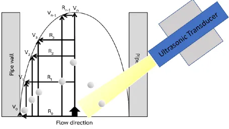
In general, the UVP system consists of a pulser/receiver, an ultrasonic transducer, and a computer, which contains signal processing methods. Ultrasonic pulses are emitted from the ultrasonic transducer with a basic frequency f0 passing through to streamline with an incident angle θω is shown in Fig. 1. Figure 1 illustrates a process of the ultrasound propagation involved in the UVP method [9]. Then, ultrasonic pulses with shift frequency fd based on the Doppler principle are reflected from the surface of particles flowing in
the fluid, and return to the ultrasonic transducer installed on the surface of pipe-wall shown Fig. 2. The Doppler-shifted frequency is directly proportional to a component VTX of the velocity V axial along the
measurement line, where cf is a sound velocity in water as follows:
2 0 C f
VTX fd
f
(1)
Hence, the UVP method can be obtained by only component along an ultrasonic path, which is one-directional flow of streamline. The velocity in axial direction Vaxial can be computed as given by
sinVTX Vaxial
f
(2)
developed in the last two decades. However, the ESPRIT Invariance Technique is far from applying it to the UVP. This research paper is the first to apply the ESPRIT to the UVP. The experimental results can guarantee that the ESPRIT was effective on flowrate measurements. Accordingly, the ESPRIT is an interesting choice of development involving the UVP. The paper is organized as follows. Section 2 describes the basis used to evaluate frequency demodulation. Section 3 introduces the ESPRIT terminology used throughout this paper. Section 4 presents the method of velocity profile measurement on single phase flow including accuracy computation. Section 5 describes the experimental framework used to evaluate the performance of the ESPRIT algorithms. Section 6 is conclusion in this paper.
Fig. 1. Structure of UVP measurement and shown the parameters for velocity profile calculation.
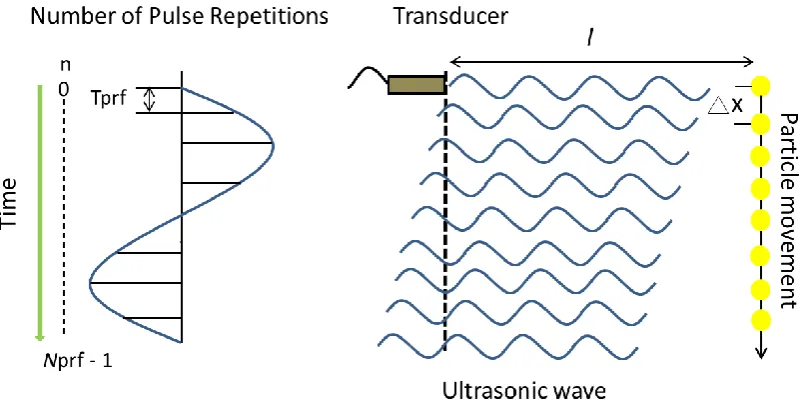
[image:3.595.125.470.191.459.2] [image:3.595.104.490.494.691.2]Fig. 3. Doppler frequency of ultrasonic waves.
2.
Frequency Demodulation Analysis
The key idea of the pulsed Doppler method is illustrated in Fig. 3. An instantaneous frequency is obtained along the ultrasonic wave. Ultrasonic waves are transmitted from the transducer with a pulse repetition frequency (fprf). The ultrasonic echo reflected from the particle is received at the same transducer. The delay
time of the ultrasonic echo is expressed as follows:
td nTprf 2l
C f
(3)
where Tprf is the time interval of the pulse repetition. The echo from the particle (s(t)) consists of an
amplitude of A, a basic frequency of f0, and a Doppler frequency of fd as follows:
( ) cos 2 0
-
d d
prf
nf
s t A f t t
f (4)
Figure 4 shows a process of the measurement system. The ultrasonic echo is sampled by an A/D device, and multiplied by the cosine and sine components. A low-pass filter is applied to the ultrasonic echo to clean up the carrier wave of f0.
2
2
0
( ) ( )exp ( ) ( )
z n s t j f t x nI ixQ n
LowPass
(5)
3.
ESPRIT: Estimation of Signal Parameters via Rotational Invariance Technique
The ESPRIT is generally applicable to a wide variety of problems for illustrative purposes on DOA estimation. The ESPRIT overcomes these problems with a dramatic reduction called shift invariance of the array [14]. Unlike most DOA estimation methods such as the multiple signal classification, the ESPRIT does not require that the array manifold steering vectors by precisely known, so the array calibration requirements are not stringent. This section explains the fundamental principle of the ESPRIT-based algorithms. Considering the parameter K = 1 and the vector of observations of xI(n) = x, when assuming
that ωk is Doppler frequency.
0 1 1 1
[ , ,..., ]
[1,exp( ),exp( 2 ),...,exp( ( 1) )] N
k k k
x x x
A j j j M
x
x
[image:4.595.98.502.84.293.2]This vector can be partitioned as follows:
Fig. 3. Schematic diagram of accurate flowrate computation.
1 0 1 2
2 1 2 1
1 2
[ , ,..., ] [ ,..., , ] exp( )
N
N N
k
x x x
x x x
j
s s
s s
(7)
Equation (7) implies that the frequency shifted between s1ands2
is ω
k. To achieve the frequency, the autocorrelation matrix due to the vector of observations can be expressed in Eq. (8).H x
x
R U U
(8)
Then, let us define two metrices including in Eq. (9).
1 ( 1) 1
1 1 1
1
M M M M M
M M
M M
1
2
I 0
0 I
(9)
They are used to select the first and last (M - 1) columns of an (M x M) matrix, respectively and called the selector matrices. We use them as follows:
1 1
2 2
S U
S U
(10)
For the matrices defined in Eq. (9), when every k denoting the different frequency components, we have:
[image:5.595.68.524.119.376.2]which can be written as:
1U
2U(12)
where
=
diag exp(
j
1),exp(j
2),...,exp(j
k)
.
The eigenvalue decomposition, namely the famous engineering tool in linear algebra, is performed using some unitary matrix T:
1 2 1 2 UT UTU U
(13)
where the superscript H is the conjugate transpose. In the first line a unitary transformation on U is applied, and in second line the property that UUH = I .
Summarizing the steps in the algorithm is:
(1) Estimate rx[k] and form Rxx of size at least K x K
(2) Calculate eigenvalue decomposition H x
x
R U U
Pick the eigenvectors corresponding to the K
largest eigenvalues and form the matrix US u1...uK(3) Solve the equation
1
2 and get 1 2H
2 2H
1
S S
U U S S S S
(4) Compute the K eigenvalues of
In the ideal case the eigenvalues are:
exp(j
k) ,
k1,2,...,KThe largest eigenvalue λk in Φ represents an estimate of the Doppler frequency factors exp(jωk)
1
arg( )
cos ( )
2 k k k d prf
f f (14)
where fprf is a frequency of repetitions which is adjusted by the pulser/receiver. The frequency is expressed
in Eq. (11), and then this frequency is plugged in Eq. (1) and (2), respectively, for creating the velocity profile.
4.
Ultrasonic Doppler Method for Flowrate Measurement
Ultrasonic Doppler method for flowrate measurement requires only a transducer whereby the measuring line goes through the center of the pipe as the simplest configuration, as shown in Fig. 3. If the flow is axially symmetric, the accurate flow rate Q(t) can be obtained accurately by integrating only the half of the velocity profile using Eq. (15), which is obtained from the measuring line going through the center of the pipe [15-16].
3 3 3 3
2
0 1 1 2
0 1
0
0 1 1 2
( ) 3
n
i i
i i n n
i i i
R R R R
Q t v v v R v
R R R R
(15)where Ri is the distance from the pipe center to the computing point, and vi is the velocity of the point.
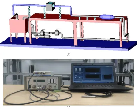
(a)
(b)
Fig. 4. Schematic illustration for a) Experimental apparatus of double pipe flow b) Ultrasonic velocity profile measurement system.
[image:7.595.76.520.83.435.2] [image:7.595.71.524.484.661.2]Fig. 6. Schematic illustration for Location of the test section.
5.
Studying Signal-to-Noise Ratio of Different Typical Noises on ESPRIT
The velocity error of each particle due to different noises was determined when the measured echo signal contained the white Gaussian noise (WGN), colored Gaussian noise (CGN), general Gaussian noise (GGN), Laplacian noise (LCN), and Gaussian mixture noise (GMN). For comparative performance, the necessary background of each noise is explained. WGN is well known in communication systems to model the ambient variance for virtually any signal processing method [16]. It has the identity distributed probability density function (PDF) pWGN, and it cannot be predicted. This is called a flat power spectrum density (PSD) PWGN shown as Eq. (16).
2 2 2
2
1 1
2
2
( ) exp [ ]
( )
WGN WGN WGN
WGN
p w w n
P f
(16)
CGN is always seen in the field of radar [17], reverberator in sonar [18], and localization in acoustics [19]. The PSD of CGN is non-flat inside the band of interest as follows
2
CGN( ) = 2
1 + 1 exp -j2
p f
a f (17)
The mathematical model defined for CGN is usually the autoregressive (AR) model, and the first order a[1] of AR was used to evaluate performance in this comparative study. GGN, as a type of non-stationary Gaussian random signal, can occur in practice because of abrupt changes [20]. A mathematical model of the PSD for GGN is given as
[image:8.595.70.526.79.356.2]where α[1,n] is a time-varying filter parameter. The two non-Gaussian PDFs, the LCN and the GMN which generate large noise spikes of noise samples, can be assumed to model such physical noise processes as man-made noise , acoustic transients [21], and geomagnetic noise [22-23] as depicted by Eq. (18) and (19).
2
2
1 2
2
( ) exp [ ]
LCN LCN WGN
p w w n (18)
2 2
2 2
2 2
1 2
1 1
1 1 1 1
1
2 2
2 2
( ) ( ) exp( [ ] exp( [ ])
GMN GMN WGN WGN
p w w n w n (19)
where ε is a mixture ratio. The indicator shows the accuracy of velocity estimate in a term of 10 log10 (1/MSE) versus signal-to-noise ratio (SNR), where MSE is the mean-squared error, as the noise power changes. The measurement position assumed that a particle was moving at a velocity of 0.1308 m/s or 500 Hz of Doppler-shift frequency, basic frequency of carrier signal was set as 4 MHz, number of pulse repetitions (Nprf) was 128, and repetition frequency (fprf) was 4 kHz. One hundred trials in five situations of noise sequence were applied. Computational results using program simulation are shown in Fig. 7. At higher SNR, the answer tended to higher accuracy while the noise power deceased. It was apparent that accuracy became lower and constant when passing approximately 20 dB.
Fig. 7. Mean-square error of velocity versus SNRs in different situations of noises: White Gaussian noise, Colored Gaussian noise with a[1] = -1, General Gaussian noise with a time-varying filter = 0.9 +n/Nprf, Laplacian noise, and Gaussian mixture noise with ε = 0.1 on ESPRIT method.
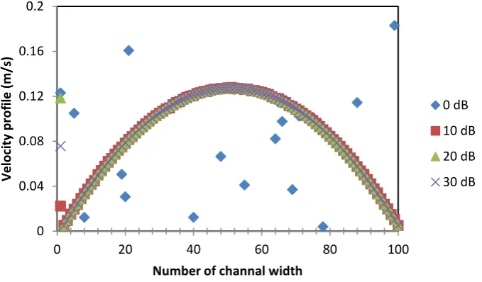
Next, velocity estimation from moving particle was computed in the flow profile equation. White Gaussian noise is undoubtedly the usual sequence that is often claimed to test the efficiency of various algorithms included in many applications. This section examined a velocity profile that was interrupted with different SNRs of white Gaussian noise. Therefore, white Gaussian noise was added to the pseudo velocity profile with SNRs of 0, 10, 20, and 30 dB. UVP under the constraint environment was evaluated by computer simulations. The situation assumed that the flowrate varied steadily at a flow constant of 12 L/min. Sound velocity traveling in water was 1480 m/s. A transducer had an angle of measurement at 45 degrees. The Nprf and Fprf were 128 and 4000 Hz, respectively. ESPRIT almost matched the true velocity
profile at noise power = 0 - 30 dB as shown in Fig. 7; however, several points of velocity were diverged from the reference at noise power = 0 dB because the velocity estimations had a huge error.
0 10 20 30 40 50 60 70
0 10 20 30 40 50
10 l
o
g
10 (1/
M
SE
)
SNR (dB)
[image:9.595.98.501.345.538.2]Fig. 8. Velocity profile estimates for 12 L/min of flowrate with different SNRs: 0 dB, 10 dB, 20 dB, and 30 dB.
Table 1. The effect of number of repetitions.
Number of repetitions
(Sample) 10 log 10(1/MSE) Accuracy
4 12
8 35
16 48
32 56
64 62
128 65
256 61
Table 2. The effect of frequency of repetitions.
Frequency of repetitions
(Hz) 10 log 10(1/MSE) Accuracy
1000 62
2000 73
3000 70
4000 68
5000 66
6000 71
7000 70
8000 63
10000 61
6.
The Effects of Number and Frequency of Repetitions on ESPRIT
Table 1 showed the effect of N
prfon the mean-squared error in the case with no noise. ESPRIT
showed similar behavior with accuracy influenced significantly by the number of recorded samples.
The eigenvalues of ESPRIT, applied to estimate the Doppler-shifted frequency, provided
reliability of computation dependent on eigenvalues contained in a matrix. For frequency of
repetitions, MSE values derived using ESPRIT with varying values of fprf are shown in Table 2. With
0 0.04 0.08 0.12 0.16 0.2
0 20 40 60 80 100
Veloc
ity
p
ro
fi
le
(
m
/s)
Number of channal width
[image:10.595.132.472.86.285.2] [image:10.595.187.410.369.483.2] [image:10.595.187.411.522.660.2]increasing fprf, the effect of MSE directly appeared in ESPRIT analysis results. ESPRIT was capable of
matching the true value for all fprf values. ESPRIT showed no fluctuation for all frequency ranges.
(a)
(b)
(c)
Fig. 9. Averaged UVP at Reynolds number = 9500 and flowrate = 20 liters/minute with varying Nprf
when fprf = 4 kHz (a) Nprf = 32 (b) Nprf =64 (c) Nprf = 128.
0 0.05 0.1 0.15 0.2 0.25
1 11 21 31 41 51 61 71 81 91 101 111
V
elocity
P
rof
ile
(m
/s)
Channel Number
0 0.05 0.1 0.15 0.2 0.25
1 11 21 31 41 51 61 71 81 91 101 111
V
elocity
P
rof
ile
(m
/s)
Channel Number
0 0.05 0.1 0.15 0.2 0.25
1 11 21 31 41 51 61 71 81 91 101 111
V
elocity
P
rof
ile
(m
/s)
[image:11.595.156.444.117.698.2](a)
(b)
[image:12.595.149.445.79.669.2](c)
Fig. 10. Averaged UVP at Reynolds number = 9500 and flowrate = 20 liters/minute with varying Nprf
when fprf = 8 kHz (a) Nprf = 32 (b) Nprf =64 (c) Nprf = 128.
7.
Experiment Results of UVP Measurement by Means of ESPRIT
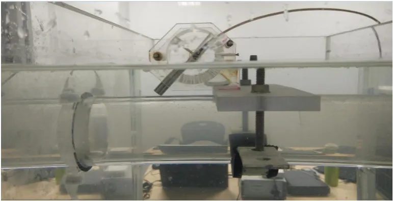
The experiment station and the developed UVP measurement package are shown in Fig.4. In Fig. 4(a), the experimental apparatus consisted of a water circulation system, a flow conditioner, a pump, a standard
0 0.05 0.1 0.15 0.2 0.25
1 11 21 31 41 51 61 71 81 91 101 111
Ve
locit
y
P
rof
ile
(m
/s
)
Channel Number
0 0.05 0.1 0.15 0.2 0.25
1 11 21 31 41 51 61 71 81 91 101 111
V
elocity
P
rof
ile
(m
/s)
Channel Number
0 0.05 0.1 0.15 0.2 0.25
1 11 21 31 41 51 61 71 81 91 101 111
Ve
locit
y
P
rof
ile
(m
/s
)
electromagnetic flowmeter, and a test section that contained an ultrasonic transducer. The station was designed to support the formation of fully developed turbulent pipe flow. Water and flowrate were circulated and controlled by a centrifugal pump. The transparent tubes of piping system are made of polyvinyl chloride (PVC). Before the test section, a flow conditioner including the tube bundle, mesh plates and a turbulent promotor ring was allocated to realize uniform velocity profiles [24]. In general, a uniform velocity profile requires a long pipe length to ensure flow characteristics. The tube bundle flow conditioner was installed at 10 times the pipe diameter (10D) upstream of the double bend to minimize flowrate measurement errors [25]. The inner diameter (D) and wall thickness of the pipeline were 50 and 5 mm, respectively. The test section was a box containing water as a couplant between the transducer and the pipe line. The couplant replaced the air to make it possible to increase sound energy into the test specimen. Figure 4(b) showed the UVP measurement package setup which consisted of four components: a 4 and 8 MHz ultrasonic probe (Imasonic), a pulser/receiver (Honda electric), an 8 bits 100 MS/s digitizer (NI USB-5133) and a personal computer which contained software MATLAB and LabVIEW. The UVP measured the velocity along the ultrasonic measuring line, so the ultrasonic probe was installed inside the test section at 45 degrees. The velocity inside the pipe wall could not be estimated due to physical limitations. This study assumed the flowrate 20 liters/minute (l/min). The condition for testing follows to Table 3. Figure 5 is a standard electromagnetic flowmeter, which was used for comparison.
The results of velocity profile were computed in a term of flowrate using ESPRIT by MATLAB program. The experimental results compared the reference with a standard electromagnetic flowmeter (Yokogawa) as shown in Fig. 5. A velocity profile of water flowrate at 20 l/min. can be shown in Figs. 9 and 10 by means of the ESPRIT. The flowrate was set at 20 L/min (Vmax = 0.22 m/s). The smallest frequency of repetitions for antialiasing was 2.37 kHz [26-27]. The pulser/receiver used in this experiment could be varied at fprf = 2, 4, and 8 kHz [28]. Accordingly, fprf was conditioned at 4 and 8 kHz because at 2
kHz fprf was aliasing. UVP was recorded by automatically repeating 1000 profiles from LABVIEW. A
central processing unit (CPU) was used for processing instructions of algorithms was assessed. In addition, elapsed time, the amount of time passing from the start of an event to its finish, was used to evaluate computation time. Intel (R) Core (TM) i5-2410 M CPU @ 2.30 GHz and Windows 7 Ultimate 64 bit operating system were used for calculation. Figures 9 (a), (b), and (c) demonstrate the experimental results of averaged UVP at a constant fprf = 4 kHz and adjusting Nprf = 32, 64, and 128. Figures 10 (a), (b), and (c)
show the experimental results of averaged UVP at a constant fprf = 8 kHz and varying Nprf = 32, 64, and 128.
The UVPs in Figs. 9 and 10 obtained the velocity profile from just after the emission of ultrasound to a setting value. Thus, the profile includes unnecessary profile, i.e. a profile in pipe walls, as well as the necessary velocity profile of the flow. The channel numbers from 0 – 10 and 110 – 120 indicated the velocity profile of the inner and outer wall sides because the velocities were approximately the zero. After that the velocity slightly increased along to more channel number. After the channel number passed 30 up to 60, the velocities reached to the maximum value according to flow characteristic, which had high velocity at the center of pipelines. All points of the UVP shown in Figs. 9 – 10 were plugged in Eq. (15) for flowrate computation. Flowrates due to Eq. (15) were compared with the standard electromagnetic flowmeter as given by Table. 4. Nprf was a main effective accuracy because ESPRIT had smaller error in order of
increasing Nprf from least to most but fprf did not.
8.
Conclusions
Development of the UVP measurement for different flowrates was executed using the ESPRIT. Double bent pipe system was used to realize the capability of the proposed idea. The measurement systems consisted of an ultrasonic pulser/receiver, an ultrasonic transducer, a digitizer, and a computer for verification. The measurement test section box was a vertical pipe made up of acrylic with an inner diameter (D) of 20 mm. The transducer was installed on pipeline with an incident angle (θ) 45o inside a transparency box containing water. Nylon tracer particles moving inside the pipeline were dispersed in water. Experimental flowrates on the system were set up for 20 liters/minute with 1000 data. The velocity profiles were obtained at the distance of upstream 16 D from the bent. The accuracy of flowrate measurements for flow characteristics by means of ESPRIT was experimentally verified. The standard electromagnetic flowmeter, which was used for comparison The ESPRIT technique for accurate flowrate measurement at the region near the bent was validated. Nprf was a main effective accuracy because ESPRIT
communication engineering, but it is applied in fluid mechanics as well. Moreover, the simulation results guarantee that ESPRIT had no effect when the five noisy signals were applied. The maximum noise intensity that ESPRIT could endure was up to 0 dB. Error of both 4 and 8 kHz of frequency of repetition was smaller than 3 %.
Table 3. Condition of Ultrasonic velocity profile measurement.
Condition Unit Value
Water flowrate Qv l/min 20
Angle θW degree 45
Pulse Repetition fprf kHz 4,8
Carrier Frequency fc MHz 4
Basic Frequency f0 MHz 4
Number of Repetition - 32, 64, 128
Number of Profiles - 1,000
Channel number - 120
Particle μm 80
Sound velocity in water m/s 1480
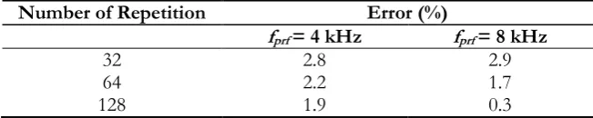
Table 4. Error of flowrate measurement obtained by means of ESPRIT at Qv = 20 l/min.
Number of Repetition Error (%)
fprf= 4 kHz fprf= 8 kHz
32 2.8 2.9
64 2.2 1.7
128 1.9 0.3
Acknowledgements
This study was undertaken following a memorandum of understanding involving research operations between King Mongkut’s University of Technology North Bangkok, Thailand and Tokyo Institute of Technology, Japan.
References
[1] M. Altendorf, Flow Handbook: A Practical Guide: Measurement Technology–Applications–Solutions, 3rd ed. Reinach: Endress + Hauser Flowtec AG, 2006, pp. 51–70.
[2] K. Tezuka, M. Mori, T. Suzuki, M. Aritomi, H. Kikura, and Y. Takeda, “Assessment of effects of pipe surface roughness and pipe elbows on the accuracy of meter factors using the ultrasonic pulse Doppler method,” J. Nucl. Sci. Technol., vol. 45, pp. 304–312, 2008.
[3] Y. Takeda, Ultrasonic Doppler Method for Velocity Profile Measurement (Fluid Dynamics and Fluid Engineering). Paul Scherrer Institute, 2010.
[4] H. Murakawa, K. Sugimoto, and N. Takenaka, “Effects of the number of pulse repetitions and noise on the velocity data from the ultrasonic pulsed Doppler method with different algorithms,” Flow Meas. Instrum., vol. 40, pp. 9-18, 2014.
[5] G. Yamanaka, H. Kikura, and M. Aritomi, “Study on the development of novel velocity profiles measurement method using ultrasonic time-domain cross-correlation,” in Proc. 3rd Symposium on
Ultrasonic Doppler Methods for Fluid Mechanics and Fluid Engineering, 2002, pp. 109–114.
[6] T. Yanagisawa, Y. Yamagishi, Y. Hamano, Y. Tasaka, K. Yano, J. Takahashi, and Y. Takeda, “Detailed investigation of thermal convection in a liquid metal under horizontal magnetic field: suppression of oscillatory flow observed by velocity profiles,” Physical Review E, vol. 82, p. 056306, 2010.
[image:14.595.154.441.166.304.2] [image:14.595.134.460.342.407.2][8] W. Wongsaroj, A. Hamdani, N. Thong-un, H. Takahashi, and H. Kikura, “Ultrasonic measurement of velocity profile on bubbly flow using Fast Fourier Transform (FFT) technique,” in IOP Conference Series: Materials Science and Engineering, 2017, vol. 249, no. 1, p. 012011.
[9] H. Murakawa, H. Kikura, and M. Aritomi, “Application of ultrasonic multi-wave method for two-phase bubbly and slug flow,” Flow. Meas. Instrum., vol. 19, pp. 205–213, 2008.
[10] Y. Takeda, “Measurement of velocity profile of mercury flow by ultrasound Doppler shift method,” J. Nucl. Sci. Technol., vol. 79, pp. 120–124, 1987.
[11] H. Dishan, “Phase error in fast Fourier transform analysis,” Mechanical System and Signal Processing, vol. 8, no. 2, pp. 113–118, 1995.
[12] N. Thong-un, W. Wongsaroj, W. Treenuson, J. Chanwutitum, and H. Kikura, “Doppler frequency estimation using maximum likelihood function for low ultrasonic velocity profile,” Acoust. Sci. & Tech., vol. 38, pp. 268–271, 2017.
[13] Z. Chen, “Introduction to direction-o-arrival estimation,” in Artech House, 2010, ch. 5, pp. 81-122. [14] R. Schmidt, “Multiple emitter location and signal parameter estimation,” IEEE Trans. Antennas Propag,
vol. 34, no. 3, pp. 276-280, Mar. 1986
[15] Y. Takeda, N. Furuichi, M. Mori, M. Aritomi, and H. Kikura, “Development of a new flow metering system using UVP,” Preliminary performanance assessment using NIST flows standards,” in ASME Fluids Engineering Division Summer Meeting, 2000.
[16] S. Wada, K. Tezuka, W. Treenuson, N. Tsuzuki, and H. Kikura, “Study on the optimal number of transducers for pipe flow rate measurement downstream of a single elbow using the ultrasonic velocity profile method,” Sci. Technol. Nucl. Ins., vol. 2012, Article ID 464313.
[17] S. Hirata and M. K. Kurosawa, “Ultrasonic distance and velocity measurement using a pair of LPM signals for cross-correlation method improvement of Doppler-shift compensation of Doppler velocity estimation,” Ultrasonics, vol. 52, pp. 873–879, Feb. 2012.
[18] F. E. Nathanson, Radar Design Principles. New Jersey: SciTech Pubs, 1999.
[19] W. S. Burdic, Underwater Acoustic Systems Analysis. Englewood Cliffs, NJ: Prentice-Hall, 1984.
[20] N. Thong-un, S. Hirata, Y. Orino, and M. K. Kurosawa, “A linearization-based method of simultaneous position and velocity measurement using ultrasonic waves,” Sens Actuator A Phys, vol. 233, pp. 480 – 499, 2015.
[21] D. Middleton and A. D. Spaulding, “Element of weak signal detection in non Gaussian environment,” in Advance in Statistical Signal Processing. Greenwich, CT: JAI Press, 1993, vol. 2, pp. 142–215.
[22] R. Dwyer, “A technique for improving detection and estimation of signals contaminated by under ice noise,” J. Acoust. Soc. Am., vol. 74, pp. 124–130, Jul. 1983.
[23] J. Schweiger, “Evaluation of geomagnetic activity in the MAD frequency band (0.04 to 0.6 Hz),” master’s thesis, Naval Postgraduate School, 1982.
[24] W. Treenuson, N. Tsuzuki,, H. Kikura,, M. Aritomi,, S. Wada, and K. Tezuka,, “Development of flow rate measurement in the bent pipe using ultrasonic velocity profile method,” in Proc. 9th International
Topical Meeting on Nuclear Thermal-Hydraulics, Operation and Safety, 2012.
[25] R. Rans “Flow conditioning and effects on accuracy for fluid flow measurement,” in Proc. 7th South
East Asia Hydrocarbon Flow Measurement Workshop, 2008.
[26] T. Ihara, H. Kikura, and Y. Takeda, “Ultrasonic velocity profiler for very low velocity field,” Flow Meas Instrum, vol. 34, pp. 127-133, 2013.
[27] H Kikura, N. Tadata, Y. Tasaka, and Y. Takeda, “A new algorithm for low velocity measurement low velocity measurement by UVP,” in Proc. International Symposium on Ultrasonic Doppler Methods for Fluid Mechanics and Fluid Engineering, 2004, pp. 121-124.

![Fig. 7. Mean-square error of velocity versus SNRs in different situations of noises: White Gaussian noise, Colored Gaussian noise with a[1] = -1, General Gaussian noise with a time-varying filter = 0.9 +n/Nprf, Laplacian noise, and Gaussian mixture noise](https://thumb-us.123doks.com/thumbv2/123dok_us/8106604.235274/9.595.98.501.345.538/different-situations-gaussian-gaussian-general-gaussian-laplacian-gaussian.webp)