Analysis of circular section blade profiles in a simple peripheral drag VAWT: design investigations and performance modelling

(1)

i

University of Southern Queensland Faculty of Health, Engineering and Sciences

Analysis of Circular Section blade

profiles in a Simple Peripheral

Drag VAWT:

Design Investigations and

Performance Modelling

A dissertation submitted by

Kristan Sedgman

in fulfilment of the requirements of

ENG4111 and 4112 Research Project

towards the degree of

Bachelor of Engineering (Honours) (Mechanical)

(2)

ii

Abstract

Global demand for off grid power generation in remote and rural locations and in low socio-economic communities has renewed interest in the use of hybrid Vertical Axis Wind Turbines (VAWTs). This type of wind turbine is more easily manufactured using simple construction techniques and materials than other wind turbine designs. They are also able to produce useable power at lower wind speeds. The use of a simple numerical modelling tool to predict the behaviour of novel hybrid Savonius and Simple Peripheral Drag (SPD) turbines would allow analysis of the performance of designs prior to construction. This would allow tailoring of a turbine design to specific local operating conditions. To enable this, investigations were undertaken to ascertain the usefulness of CFD in data generation of SPD blade performance data using ANSYS software,

correlated with wind tunnel experiments. This data was then used in a MATLAB simulation script to predict the behaviour of numerically modelled turbines using a range of variables.

(3)

iii

ENG4111 & ENG4112 Research Project

Limitations of Use

The Council of the University of Southern Queensland, its Faculty of Health, Engineering and Sciences, and the staff of the University of Southern Queensland, do not accept any responsibility for the truth, accuracy or completeness of material contained within or associated with this dissertation.

Persons using all or any part of this material do so at their own risk, and not at the risk of the Council of the University of Southern Queensland, its Faculty of Health, Engineering and Sciences or the staff of the University of Southern Queensland.

(4)

iv

Certification

I certify that the ideas, designs and experimental work, results, analyses and conclusions set out in this dissertation are entirely my own effort, except where otherwise indicated

and acknowledged.

I further certify that the work is original and has not been previously submitted for assessment in any other course or institution, except where specifically stated.

Kristan Sedgman

(5)

v

Acknowledgements

I would like to thank Dr Ray Malpress for sharing the little time and considerable knowledge he has.

I would also like to thank Mr Andreas Helwig for his inspiring conversations and for offering this interesting project for students to be a part of.

Additionally I thank the staff at the University of Southern Queensland who have assisted me over the last year, particularly Ruth Mossad, Adrian Blockland, Khalid Saleh and Prof. Andrew Wandel.

(6)

vi

List of Figures

Figure 1: Potential layout of a hybrid Savonius(bottom) and SPD (top)wind turbine cluster. ... 2 Figure 2: Idealisation of the SPD (Simple Peripheral Drag) VAWT design. ... 3 Figure 3: Some of the SPD design parameters (plan view). ... 4 Figure 4: CFD results showing the flow field around traditional (a) and Bach (b) style VAWT rotors ( Flow coloured by velocity magnitude).(Source: Zhou et.al, 2013) ... 5 Figure 5: Helical Savonius configurations showing various twist angles. (Source: Lee et. al, 2015) ... 13 Figure 6: Various end plate configurations for a helical VAWT (Source: Jeon et.al, 2014) ... 14 Figure 7: Domain for CFD analysis showing the 3 mesh size areas. ... 18 Figure 8: Meshing applied to the 3 domain regions. ... 18 Figure 9: Inflation of the boundary layer mesh from an initial cell thickness of 0.01mm to regional mesh size of 0.15mm (region C). ... 19 Figure 10: Comparison of x direction force results from the CFD analysis with wind tunnel data (CFD dashed lines, wind tunnel solid lines) at the tested wind speeds of 6.6 ms-1_{, 15.1 ms}-1_{and 20.1 ms}-1_{. ... 27}

Figure 11: Comparison of the y direction force results from the CFD analysis with wind tunnel data (CFD dashed lines, wind tunnel solid lines) at the tested wind speeds of 6.6 ms-1_{, 15.1 ms}-1_{and 20.1 ms}-1_{. ... 27}

Figure 12: Pressure fields and velocity vectors for the 180° blade at 0° offset and 180° offset angles. ... 29 Figure 13: Pressure fields and velocity vectors for the 120° blade at 0° offset and 180° offset angles. ... 30 Figure 14: Pressure fields around a 180° blade from 15° offset to 60° offset angle. At 30° and 45° vortex flow is closer to the trailing surface of the blade. ... 31 Figure 15: Plot of x direction forces from wind tunnel data interpolated over a full

revolution (180° arc solid line, 120° arc dashed line) at the tested wind speeds of 6.6 ms-1_,

15.1 ms-1_{and 20.1 ms}-1_{. ... 32}

Figure 16: Plot of y direction forces from wind tunnel data interpolated over a full

revolution (180° arc solid line, 120° arc dashed line) at the tested wind speeds of 6.6 ms-1_,

15.1 ms-1_{and 20.1 ms}-1_{. ... 32}

Figure 17: Radar plot of the net force results from wind tunnel testing (180° arc solid line, 120° arc dashed line), interpolated over a full 360° revolution. ... 33 Figure 18: Sample ANSYS fluent solution showing approximate locations of the inner three static pressure readings taken by the Pitot tube (black circles). ... 35 Figure 19: Plot of CD vs Re for (180° and 120°) blades at their maxima and minima CD

angles ... 36 Figure 20: Plot of CL vs Re for (180° and 120°) blades at their maxima and minima CL

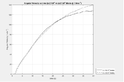
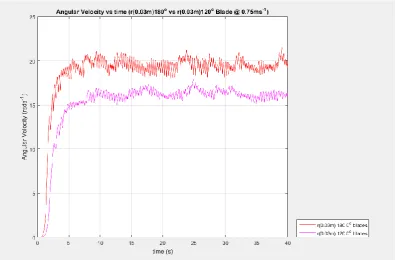
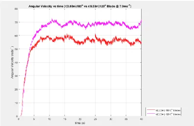
angles. ... 36 Figure 21: Angular velocity of 180° and 120° arc blades in 0.75 ms-1_{wind speed (0°}

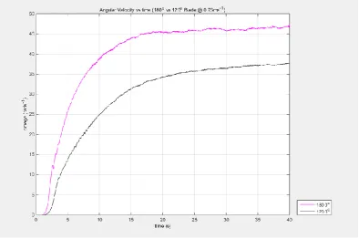
offset data used for comparison). ... 37 Figure 22: Angular velocity of 180° and 120° arc blades in 7.0 ms-1 wind speed (0° offset data used for comparison). ... 38 Figure 23: Rotational anomaly for 180° blade in 0.75 ms-1_{wind at -15° and -30° offset. 39}

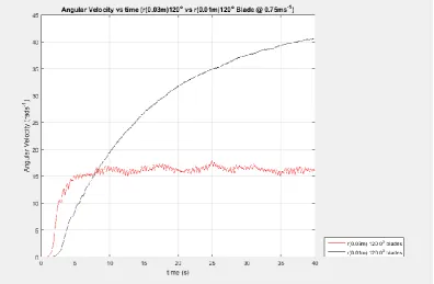
Figure 24: Comparison of rotational velocity for a three 180° bladed turbine in 0.75 ms-1

wind, showing both 0.03 m radius and a 0.01 m radius geometry. ... 40 Figure 25: Comparison of 5 and 3 bladed turbines at 0.75 ms-1_{wind speed (both 180°}

(11)

xi

Figure 28: Risk management plan image 3. ... - 4 -

Figure 33: LENS printed base and universal joint with load cells attached. ... - 9 -

Figure 34: Test specimen with graduated collar fitted (top) and complete Pitot tube and microcontroller assembly (bottom) ... - 9 -

Figure 35: Creo model ready to be transferred as an *.stl file for LENS printing. ... - 10 -

Figure 36: Test specimen with graduation collar fitted in universal joint ready for wind tunnel testing. ... - 10 -

Figure 44: Image 1 from the verification process of the jewellery scales. A range of 0.04 grams was seen between the 3 scales. This was far below the level of fluctuations experienced in the wind tunnel testing. ... - 18 -

Figure 45: Image 2 from the verification process of the jewellery scales. ... - 18 -

Figure 46: Image 3 from the verification process of the jewellery scales. ... - 19 -

Figure 47: Photograph of the testing apparatus on top of the wind tunnel test section, inlet to the left hand side of the image. The Pitot tube can be seen inserted into one of the 6 self-sealing slots available. ... - 19 -

Figure 48: Photograph of the assembled test apparatus showing the Pitot tube for pressure data acquisition (left) and a test specimen connected through to the force measurement apparatus. The static pressure reading ports on the Pitot tube are too small to be seen in this image, and are about 2cm from the tip of the tube. ... - 20 -

Figure 49: Comparison of (3) blade arc angles at 0.75 ms-1. ... - 29 -

Figure 50: Comparison of (3) blade arc angles at 7.0 ms-1 . ... - 29 -

Figure 52: Comparison of 180° vs 120° blades at 0.75 ms-1_._{... - 30 -}

Figure 54: Comparison of (120°) blade numbers at 0.75 ms-1_._{... - 31 -}

Figure 55: Comparison of (120°) blade numbers at 7.0 ms-1. ... - 32 -

Figure 56: Comparison of (180°) blade numbers at 0.75 ms-1_._{... - 32 -}

Figure 57: Comparison of (180°) blade numbers at 7.0 ms-1. ... - 33 -

Figure 58: Comparison of (120°) turbine radius at 0.75 ms-1_._{... - 33 -}

Figure 59: Comparison of (120°) turbine radius at 7.0 ms-1. ... - 34 -

Figure 60: Comparison of (180°) turbine radius at 0.75 ms-1_._{... - 34 -}

Figure 61: Comparison of (180°) turbine radius at 7.0 ms-1. ... - 35 -

Figure 62: Comparison of (0.03 m) turbine blade angle at 0.75 ms-1_._{... - 35 -}

Figure 63: Comparison of (0.03 m) blade angle at 7.0 ms-1. ... - 36 -

Figure 64: Angular acceleration of all offsets for 180° blade at 0.75 ms-1. ... - 37 -

Figure 66: Angular velocity for all offsets of 180° blade at 0.75 ms-1_._{... - 38 -}

Figure 67: Angular velocity for all offsets of 120° blade at 0.75 ms-1. ... - 38 -

Figure 68: Tip speed for all offsets of 180° blade at 0.75 ms-1. ... - 39 -

Figure 70: Comparison of angular velocity for 180° vs 120° blades at 7.0ms-1. ... - 40 -

(12)

xii

Figure 75: Tip speed for all offsets of 180° blade at 7.0 ms-1_._{... - 43 -}

Figure 77: EXCEL worksheet showing the total x and y components of force from the CFD solutions for the 180° blade at the three wind speeds tested. ... - 44 -

Figure 78: Domain of the transient solution mesh showing the three separate meshing regions. ... - 45 -

Figure 79: Image showing the three relative mesh sizes in each zone, used for the transient solution. ... - 46 -

Figure 80: Close up of the mesh around the blade surface region showing inflation from the surface, the 0.2mm rounded corners, and the triangular mesh (for the transient solution). ... - 47 -

Figure 81: Solution parameters image 1, transient setup and mesh stattistics. ... - 48 -

Figure 82: Transient solution setup using PISO scheme and the transition SST turbulence model, suitable for flows where separation of the boundary layer is apparent. ... - 49 -

Figure 83: Pressure field from transient solution showing detached vortex in low pressure (blue) region of the flow. ... - 50 -

Figure 84: Velocity field from the transient solution showing high velocity flow (red) on the lower side of the image, and lower velocity flow (blue) on the upper side of the image, with some flow back across the rear side of the blade from the vortex. ... - 50 -

Figure 85: Turbulent kinetic energy regions from the transient solution. ... - 51 -

Figure 86: EXCEL spreadsheet 1 for wind tunnel data. ... - 52 -

Figure 87: EXCEL spreadsheet showing CD and CL for various Re values. ... - 54 -

Figure 88: Plot of CD vs Re for 180° blade. ... - 55 -

Figure 89: Plot of CL vs Re for 180° blade. ... - 55 -

Figure 90: Plot of CD vs Re for 120° blade. ... - 56 -

Figure 91: Plot of CL vs Re for 120° blade. ... - 56 -

(13)

xiii

Glossary of terms

SPD: Simple Peripheral Drag VAWT: Vertical Axis Wind Turbine

Offset: angle between the centreline of a blade and the tangential vector Arc angle: internal circular arc describing the blade extent

CFD: Computational Fluid Dynamics

RANS: Reynolds Averaged Navier Stokes equations

SRANS: Steady Reynolds Averaged Navier Stokes equation y+_{: Dimensionless wall distance}

y: normal distance to wall u: time averaged velocity of flow τw: wall shear stress value

ρ: Density µ: Viscosity

uτ: wall friction velocity

Re: Reynolds number CD: Coefficient of drag

CL: Coefficient of lift

F: force m: mass a: acceleration

I: mass moment of inertia r: radius

τ: Torque

α: Angular acceleration ω: angular velocity

PISO: Pressure Implicit with Splitting of Operators SST: Shear Stress Transport

(14)

xiv FFF: Fused Filament Fabrication

LENS: Laser Engineered Net Shaping UV: Ultraviolet

PLA: Polylactic Acid

(15)

1

1. Introduction

1.1 Background

In 2013 the International Energy Agency released their “World Energy Outlook 2013” document (IEA 2013), in which they state that 1.3 Billion people around the globe live without access to electricity in their homes. This has many negative consequences, including lower than average literacy rates and health problems (Kanagawa & Nakata 2008). One study regarding the effects of access to household electrification in Madagascar (Daka & Ballet 2011) showed increased scholastic abilities in children, especially females, with associated health benefits and reduced social reproduction rates. Another study showed 82% of householders with access to off-grid electricity spent time reading in the evenings, against only 53% of householders without access to off-grid electricity (Gustavsson 2007). Researchers (Dornan & Shah) have shown that investment in modern and efficient energy generation, combined with access to this power , leads to positive economic benefits in surrounding communities.

Renewable off-grid energy production is also aligned with the University of Southern Queensland’s Food Security and Regional Resilience initiatives. These projects aim to ensure that innovation and progress in the areas of infrastructure, natural resources and agriculture allow regional Australia to remain competitive and prosperous into the future.

1.2 Aims and Objectives

(16)

2

Figure 1: Potential layout of a hybrid Savonius(bottom) and SPD (top)wind turbine cluster.

1.3 Project Scope

The project scope was to create a model that can be used to predict some of the optimum design values for a small scale wind turbine, given input parameters by a user. The type of turbine design used was nominated by one of the project supervisors to match the permanent magnet no cogging alternator design, and thus selection of turbine is not a consideration. The chosen design is a hybrid Savonius and Simple Peripheral Drag (SPD) VAWT system (fig.1), of which the Peripheral Drag components are to be investigated in this model.

Peripheral drag refers to the use of several blades of a partial circular section, arranged about the turbines axis at some distance, together producing a net torque on the turbines shaft when exposed to airflow (fig.2). Even though the peripheral drag system is not uncommon, very little literature is available describing performance characteristics or optimal configuration. Most literature relating to VAWT design addresses the Savonius and Darrieus designs, both of which fit different niches within the VAWT market. These being that the Savonius design has superior self-starting characteristics at lower wind speeds, and the Darrieus design has a higher coefficient of power at its optimum

(17)

3

Figure 2: Idealisation of the SPD (Simple Peripheral Drag) VAWT design.

The SPD system is to be incorporated into the design of this hybrid VAWT in the hope that it can increase the power production at higher tip speeds where the Savonius power curve begins to level out(Roy & Ducoin 2016), without detrimental effects at lower speeds. While not as efficient as the Darrieus design, peripheral drag components are far easier to manufacture with simple tools and materials.

The SPD system can be described by several of its design parameters, including (fig.3)…  Blade diameter (the diameter of the circular section the blade is produced from)  Blade arc (the fraction of a full circle that the blade section represents)

 Blade offset (the angle between the normal face of the blade and the tangential path of the turbine), positive offset turning the open face towards the axis.  Rotor diameter (the distance between the centre of the circular blade section and

the turbine axis of rotation)

(18)

4

Literature on the optimisation of Savonius style VAWT’s was investigated as a reference point for this study. One study of note (Zhou & Rempfer 2013) investigated the effect of blade shape on the performance of Savonius turbines, and concluded that the traditional 180°_{arc (semicircular) blade shape was not the best option for power generation, and that}

the Bach style rotor gave superior results. The results of this study indicated that some portion of the power produced by Savonius turbines was due to lift effects generated by airflow over the blades (fig.4). However it was noted that the close proximity of the blades in the Savonius layout affected the nature of the flow around the turbine, a feature not present in the SPD design.

Figure 3: Some of the SPD design parameters (plan view). Rotor radius

Blade offset Blade arc

Blade diameter

(19)

5

Figure 4: CFD results showing the flow field around traditional (a) and Bach (b) style VAWT rotors ( Flow coloured by velocity magnitude).(Source: Zhou et.al, 2013)

This discovery prompted the desire to further investigate the generation of lift effects on circular sectioned VAWT blades. In the interests of sustainable promoting sustainable resource usage, the decision was made to compare 180°_{and 120}°_{blade arcs, these}

representing whole fractions of a circular section, meaning no waste material would be generated in the construction of blades from a length of pipe.

Investigations into this phenomena were undertaken using a combination of

Computational Fluid Dynamics (CFD) software and more traditional wind tunnel testing. The flow fields around the two 180°_{and 120}°_{arcs were modelled with CFD software, and}

the resulting forces on these sections determined. This gave both qualitative and quantitative data to be examined. Wind tunnel testing of blades of the same dimensions as those used in the CFD models was then performed, to assess the level of correlation between the physical and numerical systems. These tests were carried out at a range of wind speeds and arc offsets to give a representation of the forces on the blades over a full revolution of a turbine at varying wind conditions. The data from these tests was

analysed to determine what, if any, lift effects were observable, and whether the 120°_arc

blades were suitable to be used as design components for any turbine models, or whether to abandon this variant from the rest of the project.

The next aim of the project was to create a numerical modelling program to allow prediction of a novel turbine design. Given the associated input parameters, the forces generated by airflow over the simulated blades would be determined by interpolating force values generated by CFD analysis and stored as datum values in the model. To simplify the modelling process somewhat, only the blade offset, turbine radius and wind magnitude would be variable components of this initial model. It was expected that this would allow an optimal offset angle to be determined through incremental adjustment of this variable. Once this optimal offset value was determined, other variables could be introduced to the model.

(20)

6

resources, and ensure that a design would generate the required amount of power for a particular application over the range of local wind speeds expected.

(21)

7

2. Literature Review

2.1 CFD literature review

2.1.1 Computational Fluid Dynamics

Computational Fluid Dynamics (CFD) utilizes computers to solve numerical simulations of fluid systems (Tu 2013). Several approaches have been taken towards this end, mostly characterised by the explicit or implicit equations used to solve the system. These include the Finite Element methods, Finite Difference methods, Finite Volume methods also some meshless methods (Roy & Saha 2013). Excluding the meshless methods, these all involve solving systems of differential equations relating individual adjacent nodes of a meshed system.

2.1.2 ANSYS program – equations

The ANSYS CFD program uses the finite volume method for its governing equations. The Reynolds Averaged Navier Stokes equations (RANS) are used to determine the solution to the discretised equations of the system, with various turbulence models used in addition depending on the nature of the system being modelled. These RANS equations are time averaged equation used to describe fluid flow, and particularly turbulent flows. There are numerous sources describing their derivation and use, and as such they will not be discussed any further in this paper. The turbulence models are required to complete the RANS equations, namely the fluctuating component of the flow. This program has previously been used for modelling of VAWTs, for example (Deda Altan et al. 2016) and (Shaheen et al. 2015), both studies quite similar to this one.

2.1.3 Meshing

(22)

8

2.1.4 Wall models

Special functions are often used in the regions of CFD meshes adjacent to walls to accurately capture the boundary layer effects in the flow (Tu 2013). It is important to pay special attention to the solution of this region, particularly in the case of wind turbine blades, as this is often the region of most interest. The size and inflation of the grid in this region should be assessed using the y+ _{criterion to determine its likely efficacy. The}

y+_{variable refers to the dimensionless wall distance, and is affected by the particular flow}

properties for a region of a system. Below is a description of the mathematics relating to this variable…

𝑦 = 𝑛𝑜𝑟𝑚𝑎𝑙 𝑑𝑖𝑠𝑡𝑎𝑛𝑐𝑒 𝑡𝑜 𝑡ℎ𝑒 𝑤𝑎𝑙𝑙

𝑦+_{= 𝑑𝑖𝑚𝑒𝑛𝑠𝑖𝑜𝑛𝑙𝑒𝑠𝑠 𝑤𝑎𝑙𝑙 𝑑𝑖𝑠𝑡𝑎𝑛𝑐𝑒}

𝑢 = 𝑡𝑖𝑚𝑒 𝑎𝑣𝑒𝑟𝑎𝑔𝑒𝑑 𝑣𝑒𝑙𝑜𝑐𝑖𝑡𝑦 𝑝𝑎𝑟𝑎𝑙𝑙𝑒𝑙 𝑡𝑜 𝑡ℎ𝑒 𝑤𝑎𝑙𝑙

𝜏𝑤 = 𝑤𝑎𝑙𝑙 𝑠ℎ𝑒𝑎𝑟 𝑠𝑡𝑟𝑒𝑠𝑠 𝑣𝑎𝑙𝑢𝑒

𝜌 = 𝑓𝑙𝑢𝑖𝑑 𝑑𝑒𝑛𝑠𝑖𝑡𝑦

µ = 𝑓𝑙𝑢𝑖𝑑 𝑣𝑖𝑠𝑐𝑜𝑠𝑖𝑡𝑦

𝑢_𝜏 = 𝑤𝑎𝑙𝑙 𝑓𝑟𝑖𝑐𝑡𝑖𝑜𝑛 𝑣𝑒𝑙𝑜𝑐𝑖𝑡𝑦

𝑢_𝜏 = √𝜏_𝑤⁄𝜌

𝑢+_{= 𝑢 𝑢} 𝜏

⁄

𝑦+_{= 𝑦𝜌𝑢}

𝜏⁄µ

It can be seen the y+_{variable is a function of the flow properties. Usually an iterative}

process is required to determine its value, by determining the wall shear stress from a solution, using this to find the local y+_{value and then altering the mesh size until a}

suitable y+_{value is achieved. A value of at least 1 is usually desired in the node adjacent}

to the wall. In nodes where the y+ _{is less than 5, viscous forces dominate the fluids}

behaviour, and this region is referred to as the viscous sub-layer. For y+_{values greater}

than 5 turbulent diffusion effects are encountered, and a different numerical relationship is sought. It should also be apparent that as flow behaviour changes along a surface, so too will the y+_{value, meaning grid refinement may be a lengthy procedure that needs to}

be repeated for the same surface under different conditions.

2.1.5 Turbulence in CFD

(23)

9

however with a great deal more computational resource requirements. In one study showed how turbulence model choice could affect the time taken to reach a solution. Using the Steady Reynolds Averaged Navier Stokes (SRANS) equations took 7.2 hours to solve, while LES and DES models took 120.0 hours to solve the same system (Liu & Niu 2016).

2.1.6 SST turbulence modelling

The SST turbulence model (Menter 1996) is a two equation model that differentiates between different parts of the system it is employed in. For regions adjacent to surfaces it uses the (𝑘 − 𝜀) turbulence model to more accurately predict boundary layer conditions. Further away from these regions the (𝑘 − 𝜔) turbulence model is used to stabilize the system against turbulence effects introduced by inlet conditions. The (𝑘 − 𝜀) and

(𝑘 − 𝜔) models are themselves two equation models, each using slightly different approaches to simulate turbulence effects. This results in the SST model being a four equation turbulence model, accounting for both turbulent kinetic energy (𝑘), and a scaling effects that describe the length of turbulence (ε, ω) in the different regions of the domain being studied. This turbulence model is therefore suited to flows that encounter

transitions from laminar flow regions (boundary layers) to turbulent flow regions, such as wind turbine systems.

2.1.7 Mesh independency

Mesh independency is another aspect of CFD meshing that is worth considering during any investigation into a system. One investigation into the nature of mesh independency (Almohammadi et al. 2013) noted that an independent mesh is one in which reducing the size of the elements will not affect the resulting solution. It went on to investigate how successful several different mesh independency tests were at finding this element size in a 2D system. The conclusion reached was that the success of mesh independency

determination was reliant on the nature of the system studied, and different methods may be required depending on the system at hand.

(24)

10

2.1.8 Domain

Selection of a suitable domain for a CFD study is an important decision. The domain describes the outer limits of the mesh used in the analysis, and is where boundary conditions for the study are set (Tu 2013). It is important that the boundaries for the system are far enough from the region of interest to allow convergence of the equations to an accurate solution.

2.1.9 Boundary conditions

Boundary conditions are used to define the initial values used in solution of the discretised equations for the CFD study. Typical examples of boundary conditions include constant pressure, constant velocity, constant heat flux, constant temperature and constant mass flow rate. A combination of boundary conditions is applied to at least two faces of a fluid system to describe the nature of the flow under study. Using the

properties of the fluid being studied, the governing equations of the CFD model will be solved iteratively.

After each iteration a balance of the system is taken with respect to the boundary

conditions imposed. Any imbalance in the system is shown as a residual values for each node. Values of each node are then altered between iterations in an attempt to correct for any imbalance. When the total number of iterations is reached, or the average residuals reach a predefined lower limit, the system is said to be converged. Residuals can refer to masses, forces, velocities or variables related to the governing equations used.

2.2 Wind Tunnel Literature Review

2.2.1 Wind Tunnels

Wind tunnel testing is an important tool for the study of fluid dynamics, offering the researcher the ability to control different aspects of a system systematically, and document the results of changes. In a typical scenario a test sample or object will be placed in a test section of the wind tunnel, exposed to fluid flow, and some data (qualitative or quantitative) measured. Some commonly utilised variables include velocity of the fluid (air) stream, angle of the test sample relative to the airflow direction, and shape of the test sample.

2.2.2 Tunnel types

(25)

11

conjunction with a closed test section, this also allows for conditioning of the fluid, for example, changing the pressure above or below atmospheric pressure, changing the fluid temperature, or using non atmospheric gases. One distinct drawback of a recirculating wind tunnel is the larger volume required to extend the tunnel into a loop.

Single pass wind tunnels do not re-use exhaust air from the test section, and instead simply discharge the exhaust to the atmosphere. They require a smaller footprint than the recirculating tunnel model, and cannot modify fluid properties beyond the mass flowrate through the test section. Despite this, their relative simplicity of design and lower cost make them an attractive option where atmospheric flow is the primary fluid regime of interest.

2.2.3 Inlet considerations

Both wind tunnel types are required to condition the fluid flow entering the test section to some degree. It is generally preferable to have a uniform laminar flow field through the test section of the tunnel. In some cases it is necessary to account for a minimal, or prescribed, amount of turbulence in the flow. Commonly this is achieved by using a converging section at the inlet of the test section, with an interface structure across the tunnel to encourage either laminar flow, or flow with a predetermined amount of turbulence. This could be as simple as a section of wire mesh across the tunnel.

2.2.4 Test section considerations

The test section may be one of two general types, closed or open. Closed test sections are bounded by walls to restrict all flow to the cross sectional area of the test section, while open test sections have no walls, and allow flow to interact somewhat with the local atmospheric conditions. Open test sections are often used when a test sample is large relative to the test section, and blockage effects need to be reduced.

2.2.5 Blockage effects

Blockage effects are (typically unwanted) effects caused by incompressible fluid flow between an object and the bounding walls of the test section. As per Bernoulli’s

hypothesis, the reduced area that the incompressible flow has available to it either side of the test specimen causes changes in the flows characteristics. As the mass flowrate must be the same through all sections of the tunnel, the flow velocity will increase around the test specimen. After passing the specimen the area available to the flow increases again, and some pressure differential may result as part of the flow reduces velocity.

The effect of this is that the flow interacting with a test specimen is different from the flow introduced into the inlet of the wind tunnel. Pressure differentials that are not present in the real system will skew the results obtained from the test. Also, a flow modelled at, for example, 10 ms-1_{, will actually interact with the test specimen at 12 ms}-1_,

(26)

12

There has been quite a bit of literature devoted to quantifying the effects of blockage in wind tunnels, and how to deal with it. One review of blockage correction (Ross & Altman 2011) studied several different blockage correction methods. It found that further research is necessary to determine a definitive correction strategy, as no single strategy could account for all situations posed. The conclusion was reached that awareness of blockage effects is an important consideration when designing and analysing

experimental procedures. The same study also drew attention to the difference in blockage effects between static and dynamic models of the same geometry and instantaneous orientation to the flow.

A more specific study on blockage effects in an open test section (Roy & Saha 2014) concluded that blockage ratio and wind speed values were not sufficient to determine the required blockage correction for different tip speed ratios and torque values of a Savonius turbine. However, it notes that for small blockage ratios (less than 10%) in open test sections, the blockage correction required is negligible. For closed sections a blockage ratio of 2.0% to 3.5% has been deemed small enough to give negligible blockage effects (Ross & Altman 2011).

2.2.6 Measurement methods

Data that may be taken from wind tunnel test includes  Flow velocities

 Pressure values  Force values

 Turbulence intensity  Temperatures  Vorticity

The data of interest to this project was the forces experienced by the test specimen, however pressure and velocity measurements were also used to attempt a correlation between the wind tunnel test data and the CFD predictions. Details of the exact

measurement techniques employed is covered in the methodology section of this report.

2.3 VAWT Literature Review

2.3.1 Vertical Axis Wind Turbines

Vertical Axis Wind Turbines have received renewed interest due to increasing awareness of the environmental impact of fossil fuel use for power generation and rising energy resource costs for consumers. This increase interest has been driven by the evolution of materials and production techniques during the latter part of the 20th_{century (Tjiu et al.}

(27)

13

Research into improving the self-starting characteristics of the Savonius type VAWTs, one of their major advantages, has led to the concept of using multiple stacked units, as well as investigations into the optimum number of buckets per rotor (Sheldahl et al. 1978). These small alterations have contributed a significant increase in the effectiveness of Savonius type VAWTs in low wind speed conditions. Another study (Shaheen et al. 2015) have investigated the increase in performance resulting from selective placement of adjacent Savonius turbines within close proximity to one another. This study noted a 34% increase in the power co-efficient of clustered Savonius VAWTs compared to isolated units, due to the interaction of the flow field amongst the clustered units.

Advances in manufacturing techniques have enabled researchers to investigate the use of helical shaped Savonius buckets (fig.5). Turbines utilising this blade shape enjoy smoother power delivery compared to the traditional straight bucket turbines, as well as improved self-starting characteristics (Saha & Rajkumar 2006), with a twist angle of 15° from the vertical axis of revolution found to give optimum results in terms of the rotors performance. It should be noted that the construction of helical buckets may require more technical effort than using simple straight buckets.

Figure 5: Helical Savonius configurations showing various twist angles. (Source: Lee et. al, 2015)

(28)

14

sides, and therefore increasing the useful momentum transfer from the oncoming air stream.

Figure 6: Various end plate configurations for a helical VAWT (Source: Jeon et.al, 2014)

It is widely noted in the literature that the relative positioning of Savonius buckets to one another has a large effect on the performance of the turbine. The overlap ratio between the inner edges of the buckets on a 2 rotor Savonius turbine has been determined to give maximum efficiency at an overlap ratio of 0.15 (Akwa et al. 2012). This was due to the flow of air between the advancing and retreating buckets, reducing the pressure difference across the advancing blade.

Research into SPD type VAWTs was sparse, only literature that was non peer reviewed could be found by the author. This is probably due to the better performance of Darrieus and Savonius VAWTS and the resulting interest in them by both academia and industry. Nevertheless, it seems likely that some of the research methods applied to Savonius rotors is applicable to SPD designs. This is due to the probable similarities in flow

(29)

15

2.4 Additive Manufacture Literature Review

2.4.1 Additive manufacture

Additive Manufacture, also referred to as 3D printing or stereolithography, is the process of forming a structure by successive addition of layers of a construction material. This process results in the ability to form constructs that other more traditional subtractive fabrication methods are unable to replicate. There are many different methods and materials used to form these layers, with a range of mechanical properties and economic considerations. Two additive manufacturing methods were available for use in this project. Fused Filament Fabrication (FFF) in the form of heated polymer filaments, and Laser Engineered Net Shaping (LENS) utilizing a UV laser cured resin.

The FFF machines used either Polylactic Acid (PLA) or Acrylonitrile Butadiene Styrene (ABS) filaments. Investigation in to the mechanical properties of components

manufactured using PLA (Farah et al.) has determined a maximum tensile stress in samples of 60 MPa immediately after manufacture, reducing to 40 MPa after 3 months of ageing. Another study (Dawoud et al. 2016) determined a maximum tensile strength for ABS printed components of 34.3 MPa, however it noted that this value was higher in injection moulded processes.

The available FFF units available were the UPBOX and UPBOX mini, capable of 0.1 mm vertical layer thickness at maximum resolution (UP3D 2015). Thicker layers were possible, resulting in a decrease in production time, but with an associated increase in surface roughness. This roughness is due to the thickness of the individual layers of deposited material, and their tendency to “squash out” at the sides of the print. PLA prints can be surface treated after deposition to decrease this roughness by soaking in an acetone vapour bath. The acetone vapour partially melts the outer surface of the printed item, allowing the individual layer edges to run together. This process also increases the durability of the printed object, reducing the number of surface defects that may initiate fracture under strain.

The LENS UV curing machine available was a ProJet® 3500 HD. In its highest

resolution this machine will produce items with a thickness resolution of 0.032mm. The manufacturing process for this type of printer does not use extruded material, but rather focused UV laser light. The light produces a reaction in a UV sensitive resin, which then hardens into a solid. To allow cavities to be produced, a second material can be printed alongside the resin, a wax which melts above 60 °_{C. The ProJet printer available was}

equipped with a proprietary resin, namely VisiJet® M3 Crystal. When cured, this material exhibits a tensile strength of 42.4 MPa (3dsystems 2015). Total possible build size for the ProJet machine is 298 mmx 185 mm x 203 mm (xyz).

(30)

16

After consideration of the options, the UV curing printer was selected for production of some of the data collection apparatus. Its ability to deliver components with acceptable mechanical properties at the highest resolution was the deciding factor. This would allow the use of small air galleries for pressure measurement, and the ability to mate

(31)

17

3. Methodology

3.1 CFD Methodology

3.1.1 Geometry

The geometry used in the CFD modelling was created using the ANSYS Designmodeler package. The simulation was run as a 2D model to reduce computational time restraints, a practice not uncommon in CFD analysis (Almohammadi et al. 2013). The domain of the study was modelled as a rectangular representation of the test section of the wind tunnel, intersecting the centre of the test blade horizontally, with the domain extending five times the diameter of the test blade upwards of the blade, ten times downwind, and five time either side (fig.7).

The test blades were modelled as 20mm outside diameter with 1mm wall thickness, matching the test blades used in the wind tunnel tests. The sections were divided with a radial line originating at the centre of the circle. Early meshes indicated that sharp edges around the corners of the blade caused problems, with poor convergence of the solution. For this reason 0.2mm radii were introduced to the corners of the model where the circular faces met the radial intersecting faces see (fig.9).

For each incremental angle tested, the radial lines were redefined in the Designmodeler geometry, resulting in a change in the apparent offset angle of the test blade around the centre of the 20mm diameter. One of the radial lines was designated as the “offset” angle, while the other radial line was set as a fixed angle from the offset line, keeping the arc of the blade at the set 120°_{or 180}°_{required for the model. The offset angle was}

redefined as a parameter, while the arc angle was not changed. This resulted in an axis of rotation offset from the axis of rotation of the physical test blade. This small detail would have no appreciable difference in the results, and was done for convenience after

problems modelling the CFD blade rotation about the blade surface.

3.1.2 Meshing

(32)

18

Figure 7: Domain for CFD analysis showing the 3 mesh size areas.

Figure 8: Meshing applied to the 3 domain regions.

Region A had the largest resolution applied to it, as the flow here had very little relevance to the region of interest around the SPD blade representation. A maximum face size of 5mm was prescribed for this region. The cell behaviour was set to soft to allow smooth adaptation between region A and region B’s cell sizes. The upper and lower walls had a default edge sizing applied with a local minimum size of 5mm. The inlet boundary was located on the left-most face of region A.

Region B was an intermediary region included to allow a more gradual reduction in mesh size towards the blade. The flow in this region was expected to be less linear than region A, however as it was not in contact with the blade surface the maximum cell size was decreased to a value of 0.35mm. The right-most face of region B formed the central region of the outlet boundary.

Region C was the innermost portion of the domain, and contained the blade surfaces. As such it was given the smallest mesh size. A maximum face size of 0.15mm was used to capture as closely as reasonably possible all the flow dynamics in the air around the SPD

A

B C

A

C

(33)

19

blade surface. The outer border of region C where it met region B was given an edge sizing constraint of 0.15mm.

The SPD blade surface located in region C was given an edge sizing constraint of

0.05mm across its entire length. This was selected after numerous meshing attempts, and seemed to give reasonable results in terms of node spacing across the rounded corners of the surface. An inflation parameter was set in region C to allow inflation of the surface cells from an initial cell thickness (normal to the surface) of 0.01mm, through a

maximum of 14 layers, each with a 1.2 times growth rate. This resulted in a region of mesh modelling the boundary layer of approximately 0.8mm thickness (fig 9).

Figure 9: Inflation of the boundary layer mesh from an initial cell thickness of 0.01mm to regional mesh size of 0.15mm (region C).

3.1.3 Mesh Independency process

The grid independency study focused on region C, where higher resolution of flow characteristics was required. Force results for the SPD blade surface were used as a datum for the grid independency study. The meshing started at a maximum face size of 2mm, reducing in size until the maximum face size reached 0.15mm. At this point the mesh size was deemed accurate enough for this study.

It should be noted that the results obtained from the grid reduction process do not indicate that grid independency was actually achieved. Force results on the blade surface were still not stable, however the limits of reasonable computational time had been reached. The mesh size reduction did result in a decrease in the difference between the CFD blade force results and the wind tunnel test blade force results. This was taken to indicate that the mesh size reduction had indeed improved the accuracy of the CFD results, albeit not to the level that was sought originally.

The final meshes that resulted from the grid independency study had approximately 650,000 nodes (fig.8), depending on the actual blade arc angle and blade offset angle of each iteration. As the initial 180° CFD results had produced unusable results, only three 120°_{arc angle meshes were created, at 0}°_{, 90}°_{and 180}°_{offset angles. These were purely}

to correlate the CFD results with the wind tunnel results for completeness. A total of 42 meshes were created.

(34)

20

3.1.4 Solution discovery

The Transition SST model was used for solving the meshes generated, with all variables left at the default settings

For all solutions the boundary conditions for the analyses were set as a constant flow velocity at the inlet boundary, and a zero gauge pressure on the outlet boundary. The flow velocities determined by the wind tunnel tests were used (6.6ms-1_{, 15.1ms}-1_and

20.1ms-1_{) for each mesh. This resulted in 126 solutions being calculated. For each}

solution the x and y direction force values on the SPD blade surface were written to a data file. A separate data file was created to contain images from the solutions.

Each solution had three images recorded from the CFD-post package on the ANSYS workbench. One showed the pressure field around the SPD blade. This was to be used qualitatively in reference to the other solutions, as well as quantitatively in reference to the static pressure recordings from the wind tunnel tests. Another image was recorded showing the predicted flow velocities around the SPD blade, to be used purely as a qualitative reference. The third image showed the pressure distribution field overlayed with the flow velocities, again purely for qualitative analysis.

3.2 Wind Tunnel Testing Methodology

3.2.1 Tunnel Information

The wind tunnel used for testing of the prototypes is a single pass type driven by a fixed speed electric motor connected to a centrifugal air pump. In operation the centrifugal pump draws air from its inlet adjacent to the test section of the tunnel, and expels this air through a baffle to the atmosphere. The electric motor and air pump are mounted to a sliding base that can be manually moved using a hand screw, allowing them to be moved axially in relation to the test section. This regulates an amount of air that can be drawn into the pump directly from the atmosphere instead of via the test section. The result is adjustable flow through the test section with constant electric motor speed.

The test section itself has a 310mm x 310mm square cross section, 590 mm in length. The test section walls are constructed of 10mm thick Acrylic sheets, allowing visual observation of the test section interior. A removable top wall allows modification and replacement of mounting equipment easily. The test section is fed by a fibreglass inlet housing that gradually decreases in square cross sectional area towards the test section. This, combined with two layers of wire mesh screening, provides an air flow into the test section with minimised turbulence.

(35)

21

3.2.2 Test Apparatus

Test forces were measured using a pivoted hollow cylindrical brass lever. One end of the tube was rigidly attached to the brass test blade using silver solder. The other end was attached to the external force testing rig through a 10mm hole in a 12mm thick marine ply board which formed the roof of the test section. This rig consisted of 3D printed

components forming a central universal joint and surrounding support frame. The inner portion of the universal joint was extended to form a two part clamping structure. This structure allowed graduated rotation of the brass tube and test blade relative to the air stream, as well as the transmission of the forces to the measurement devices. The surrounding support frame included mounting points for the force measuring devices (Appendix B2).

The measuring devices were three 0g-200g jewellery scales, which gave measurements to two decimal places. With their cases cut in half to reduce their size, the load cells and measurement plates were detached and mounted to the force test rig frame. The load cells were tested against each other before the test using a nut and bolt, and some slight variation in the weights measured was noted (Appendix C2). The load cells were mounted vertically on the frame, and the measured forces were transmitted normal to their surfaces.

A Pitot tube was used for the pressure measurements. It was purchased from a hobby supplies company, and is designed for use with radio controlled aircraft. The pressure from its static and stagnation ports was transferred by the pressure probe apparatus to a Bosch BMP280 barometric pressure sensor, interfaced using an Arduino ATmega

microcontroller board. The sensor output an absolute barometric pressure reading every 3 seconds, averaged over the last two readings to reduce noise. This data was recorded via a serial monitor. Two pressure readings (static and stagnation) were used to determine the airstream velocity at a point upstream of the test specimen. The static line was also used to measure the static air pressure data behind the test specimen. Pitot tube, pressure lines, breadboard with the sensors attached and microcontroller were assembled into a single unit using 3D printed components (Appendix B3). Small covers were required to cover the pressure sensors, as they are sensitive to the effects of light. The Pitot tube could be placed through the marine ply roof at various locations (Appendix C3), and when removed rubber covers would seal the slots to prevent unwanted air flow into the test section.

The Pitot tube uses Bernoulli’s equation to determine the velocity of a moving air stream my comparing its static and stagnation air pressures. Bernoulli’s equation is re-arranged as below to allow determination of the velocity of an incompressible fluid flow. Here we will consider data denoted with subscript 1 as the static stream values and those denoted with a subscript 2 as the stagnation values.

Bernoulli’s Equation for incompressible, frictionless flow neglecting viscous effects:

𝑣₁2

2 + 𝑔. 𝑧1+ 𝑝₁

𝜌 = 𝑣₂2

2 + 𝑔. 𝑧2+ 𝑝₂

𝜌

From this, the second term of each side relating to difference in height can be ignored in this case, giving…

𝑣12

2 +

𝑝1

𝜌 = 𝑣22

2 +

𝑝2

(36)

22

As the stagnation pressure is found when the velocity of the fluid is zero, the equation simplifies again to…

𝑣₁2

2 +

𝑝₁

𝜌 =

𝑝₂ 𝜌

Next rearrange to determine the velocity of the fluid in question…

𝑣₁= √ 2 ∗ (𝑝2− 𝑝1) 𝜌

The test blade shows a maximum frontal section at 0°_{and 180}°_{offset angle, totalling 1200}

mm2_{. The test section of the wind tunnel has a total cross sectional area of 96,100 mm}2_.

This results in a maximum blockage ratio for the wind tunnel test of approximately 1.25%. Although this does not take into account the additional frontal section of the brass tube, very little blockage effects would be expected. Therefore it was not deemed necessary for the data collected in the static blade tests to be treated with any blockage correction factors.

3.2.3 Testing Procedure

The purpose of the wind tunnel testing was to correlate predicted flow characteristics and resulting forces on the test blades with data predicted by the CFD model. The two test models were tested at 30°_{increments from 0}°_{offset angle from the airflow to 180}°_offset

angle. Each of these 7 angular increments was tested at 3 wind speeds. The lowest wind speed attainable for the wind tunnel was 6.6 ms-1_{and thus was used as the lowest test}

wind speed. At a wind speed of 20.1 ms-1_{the measuring equipment reached its maximum}

operating load of 200g, and thus this was used as the largest wind speed. An intermediate wind speed of 15.1 ms-1_{was chosen to complete the testing regime.}

The wind tunnel tests performed measured two variables to compare with the CFD model. Force against the test blade was measured in both the tangential flow direction and normal to the flow in the horizontal plane, at all wind speeds and blade orientations. In addition to this the static air pressure was recorded at five different locations behind the test blade. The locations measured were on the central horizontal plane of the test section, at 0mm, 50mm and 100mm either side of the centre of the test specimen, and 30mm behind it.

The static air pressures were recorded to compare to the pressure distribution predicted by the CFD model. This was to be quantitative in the actual pressure value comparisons, as well as providing a qualitative interpretation of the pressure profile across this section of the tunnel. Unfortunately, due to the 3 dimensional nature of the flow in this region, measurement of flow velocities was deemed too difficult to attempt.

(37)

23

1. Multiply the value displayed by the load cell by the gravitational constant 9.81 ms-1_{to convert the mass to a force value as per Newton’s second law}𝐹 = 𝑚 ∗ 𝑎

, the scales having already converted the force value to a mass interpolation. 2. Use the lever function

𝐹_𝑎𝑟𝑚∗ 𝑥_𝑎𝑟𝑚= 𝐹_𝑟𝑖𝑔∗ 𝑥_𝑟𝑖𝑔 𝑡ℎ𝑒𝑟𝑒𝑓𝑜𝑟𝑒 𝐹_𝑎𝑟𝑚 =𝐹𝑟𝑖𝑔∗𝑥𝑟𝑖𝑔

𝑥𝑎𝑟𝑚

to determine the force being generated by the test blade and the brass tube it was anchored to.

3. Subtract the drag force generated by the brass tube at that wind speed (experimentally determined).

4. Divide the resulting force by the length of the test blade to give a force per millimetre value, the same as the data supplied by the Fluent CFD package.

3.3 Additive Manufacturing Methodology

The Additive manufacturing process began with 3D modelling of the test rig components required for testing. CREO parametric 3.0 was chosen due to its availability and the author’s recent experience with its use. The individual parts of the testing apparatus that needed to be printed were identified and modelled. These individual models were then arranged into assemblies to allow printing of all parts via a single file (Appendix B4). Next, the assemblies were saved as standard tessellation files (*.stl) and transferred to the LENS printer software. The files were smoothed to reduce the size of the tessellations, converted to machine code and then printed.

The completed components were transferred to an oven where they were heated to approximately 60°C to melt the support wax. They were then transferred to an ultrasonic oil bath to assist the removal of wax from some of the smaller galleries in the parts. Any parts that still had wax blockages in their small galleries were heated in a hot water bath to 60°C and compressed air was used to force the liquid wax out. Surfaces that would be used with adhesives, such as the Pitot tube support, were wiped clean and roughened slightly with sandpaper to ensure complete wax removal and assist adhesion. The test apparatus components were then assembled (Appendix B5).

3.4 MATLAB Methodology

MATLAB was used to derive predicted behaviour of novel turbines using the wind tunnel results saved in excel spreadsheets. The algorithm (Appendix D1) used this data, loaded as .csv files, and a range of user defined variables to perform the calculations. User defined data included…

(38)

24

Two wind speeds were used for the simulations, one set at 0.75 ms-1_{and another at 7ms}-1_.

This was done to determine the different responses for low and high wind speeds. Similitude to a scaled prototype was not considered when choosing the test wind speeds. Two turbine radius values were used, one at 0.01m and another at 0.03 m. The purpose of these values was to analyse the different behaviours to be expected when altering the radius of a prototype turbine. The wind speeds were simulated using turbines with 3 blades.

Offset range were tested in 15° increments from -30° through to 45°. Any changes in performance either side of the neutral offset could then be determined. The offset range was chosen arbitrarily based on a belief by the author that angling the open face of the blade towards the axis of revolution would be more beneficial, hence the slight bias in this direction.

Turbines with 3 blades were tested as well as turbines with 5 blades. This was done to assess the effect of altering the number of blades with respect to turbine performance. Both of these simulations were performed at both trial wind speeds. The results from each turbine were analysed with respect to each other at each wind speed, as well as between the same turbine designs at the different wind speeds.

Other variables were common to all simulations, and as such were not considered to be user defined as such. These included…

 Blade type (180° and 120° arc)  Duration of simulation

 Time step of simulation  Rotational inertia of turbine

The time step used for the simulations was determined after considering the time that the simulations would require to run, the amount of memory of the computer used to run the simulations, and the accuracy of the results determined by the simulation. After several trials a time step of 0.0002 seconds was determined to give results that seemed

reasonably stable, and kept computational time to a reasonable level. Duration of each simulation was limited to 40 seconds, at which point most of the results had become relatively stable.

Each simulation that was run gave the following data sets. Time_data_1

 Incremental time step values for 180° blade  180° blade angular acceleration at each time step  180° blade angular velocity at each time step  180° blade tip speed at each time step Time_data_2

(39)

25

The rotational inertia value used was aimed at a likely value for a wind tunnel prototype. The design was idealized as a simplified hoop mass, with a mass of 200g, radius to the centre of mass 0.02m. Using the formula for rotational inertia of a hoop mass

𝐼 = 𝑚 ∗ 𝑟2 _{= 0.2 ∗ 0.02}2_{= 0.00008 𝑘𝑔𝑚}2

(40)

26

4. Results

4.1.1 CFD results

From the solutions to the CFD analyses performed, force values on the turbine blade surface were determined by the ANSYS software. This was recorded in the form of x and y vector components of the net surface forces on the model (APPENDIX E1), x being parallel to the fluid stream direction, y being normal to the fluid stream direction, in the 2D model. The force values were given in units of Nmm-1_{, indicating a total force}

exerted on an extruded surface formed by the blade section modelled, per mm of extrusion. These data points were compared to the analogous wind tunnel test data. The CFD data points were not correlated by the wind tunnel force data through the entire range of angles tested. The force vectors of the CFD predictions in the x direction all showed a maximum value at 30°_{, and a smaller maxima at 120}°_{offset angle (fig.10). The}

force data points in the y direction were erratic, with multiple maxima in the positive and negative tenses (fig.11).

The x direction forces predicted by the CFD analysis had a maximum deviation from the wind tunnel data at 30° rotation, over predicting the force by 312% in the 20.1 ms-1

analysis. The second major deviation at 135° rotation over predicted the force by 174%. This pattern was observed for all three wind speeds analysed.

The y direction forces predicted by the CFD analysis showed erratic over prediction of the magnitude of forces measured in the wind tunnel tests. The maximum deviation was 5.7 Nmm-1_{in the 20.1 ms}-1_{analysis of the 150° rotation mesh. As with the x direction}

(41)

27

Figure 10: Comparison of x direction force results from the CFD analysis with wind tunnel data (CFD dashed lines, wind tunnel solid lines) at the tested wind speeds of 6.6 ms-1_{, 15.1 ms}-1_{and 20.1 ms}-1_.

Figure 11: Comparison of the y direction force results from the CFD analysis with wind tunnel data (CFD dashed lines, wind tunnel solid lines) at the tested wind speeds of 6.6 ms-1_{, 15.1 ms}-1_{and 20.1 ms}-1_.

0

5

10

15

20

0

30

60

90 120 150 180

For

ce

(N/

mm)

Offset angle (0-180 degrees)

X direction forces: Wind tunnel

data vs CFD predictions (180

º

arc

)

wind tunnel X @ 6.6 m/s

wind tunnel x @ 15.1 m/s

wind tunnel X @ 20.1 m/s

cfd X @ 6.6 m/s

cfd X @ 15.1 m/s

cfd X @ 20.1 m/s

-10

-5

0

5

10

0

30

60

90 120 150 180

for

ces

(

N/

mm)

offset angle (0-180 degrees)

Y direction force: Wind tunnel

data vs CFD predictions (180

º

arc

)

wind tunnel Y @ 6.6 m/s

wind tunnel Y @ 15.1 m/s

wind tunnel Y @ 20.1 m/s

cfd Y @ 6.6 m/s

cfd Y @ 15.1 m/s

(42)

28

After the comparison of these unexpected results from the CFD analysis, further research was conducted. Discussion with peers revealed that use of a steady state model for the ANSYS solution may have resulted in the large deviations observed. It was suggested to the author that use of a transient solution was probably warranted. A targeted literature review into ANSYS methodology used in similar research found agreeable results. In the course of research in Darrieus Turbine modelling (Lanzafame et al. 2014), it was determined that the use of a transient solution was required for accurate results. This same study also found that a PISO (Pressure Implicit with Splitting of Operators) solution approach gave better accuracy, and that calibration of the Transition SST variables for the turbulence model was necessary. Using this approach the authors found a good

correlation between CFD and experimental data.

A second attempt at CFD analysis was conducted using this information as a guideline. The domain of a 2D CFD analysis was meshed for a 180° arc blade at an offset of 30°. The face of the domain was split into three zones (Appendix E2), the smallest one

surrounding the blade, an intermediate one surrounding the first and the third representing the remainder of the domain. The innermost zone (A) of the mesh surrounding the blade was given a maximum face size of 0.10 mm, the intermediate zone (B) a maximum face size of 0.35 mm, and the outer zone (C) a maximum face size of 7 mm. A triangular mesh was used for all three zones (Appendix E3). An inflation was applied to the mesh on the surface of the blade to capture the boundary layer flow Appendix D4).

The inlet condition for the analysis was set as a 20.1 ms-1 flow velocity, with a zero gauge pressure outlet condition. The PISO scheme was used and a transient time step of 0.02 seconds was applied over a series of 50 time steps (Appendix E5). The resulting analysis required approximately 4 hours to solve. The force results indicated the same 16.3 Nmm-1 in the x direction, and 16.2 Nmm-1 force in the negative y direction, an even larger deviation from the wind tunnel data acquired. The flow showed some similarity with the original solution (Appendix E6), however the trailing vortex was detached from the blade surface (Appendix E7), with several regions of turbulent kinetic vortices (Appendix E8).

4.1.2 CFD Results Discussion

The CFD results obtained are of no use in modelling due to their large deviation from physical test data for the same system. The erratic nature of the y force data in particular would likely lead to spurious results in any MATLAB model. The poor data may have been due to one of several causes, poor meshing, poor numerical model selection, or boundary posing problems.

While a mesh independency study was attempted for the initial CFD models, it was not completed due to restriction of computational power and time constraints. To determine the independency of a mesh used for analysis it would be necessary to iteratively reduce the node sizing of a mesh, use the solver to determine a solution, and compare a monitor value such